analysis of a premature rupture of a stellite weld on a P91 valve used in a powerplant. For all ... Numerical heat transfer. â Fluid flow (CFD) .... droplets and gas, implemented in the free software ..... by integrated modelling: A maintenance inspection of a ..... in friction stir weldingâ Science and Technology of Welding and.
International Review of Chemical Engineering (I.RE.CH.E.), Vol. 2, N. 1, January 2010 Special Section on 1st Conference on Chemical Engineering and Advanced Materials (CEAM) VIRTUAL FORUM
Integrated Multiphysics Modeling in Materials and Manufacturing Processes J. H. Hattel Abstract – Today, multiphysics modelling of single process steps as well as modelling of entire process sequences and the subsequent in-service conditions are areas which increasingly support optimization of manufactured parts. In the present paper two different examples of modelling manufacturing processes from the viewpoint of combined materials and process modelling are presented: i) Integrated modelling of spray forming and ii) Integrated multiphyics modelling of friction stir welding. The third example describes integrated modelling applied to a failure analysis of a premature rupture of a stellite weld on a P91 valve used in a powerplant. For all three examples, the focus is put on modelling results rather than describing the models in detail. Comparison with experimental work is given in all examples for model validation as well as relevant references to the original work. Copyright © 2010 Praise Worthy Prize S.r.l. - All rights reserved.
Keywords: Integrated Modeling, Multiphysics, Spray Forming, Friction Stir Welding, Failure Analysis
I.
Introduction
In the field of manufacturing engineering it has become more and more evident that computer simulation is a must in the search for optimised products and structures. Today, complex thermal manufacturing processes such as casting and welding are often addressed with multiphysics models involving both Computational Fluid Dynamics (CFD) and Computational Solid Mechanics (CSM) as well as thermodynamic and kinetic models, see e.g. [1]-[6]. Recently, multiphysics modelling of welding has also been combined with optimization methods to achieve desired properties of the weld; e.g. Mishra et al. [7] make an optimization of the weld geometry with multiphysics modelling in combination with genetic optimization algorithms. In addition to this, the integration of multiprocess steps and materials modelling has emerged as a new growing field which attracts some attention in literature, although, the amount of articles dealing specifically with the subject is still relatively limited. Crumbach et al. [8] make a through process modelling of aluminium sheet production following the microstructural evolution during the production steps involving casting, heat treatment and forming processes. Also Bellini et al. [9] analyse the heat treatment of cast parts. Kermanpur et al. [10] simulate the various stages of gas turbine disc manufacture to track defects throughout the entire process chain of melting, homogenisation heat treatment, cogging, forging, final heat treatment and machining. Gandin et al. [11] make an integrated model of casting,
solidification and heat treatment in order to predict the final yield stress of an Al-Cu cast alloy. Myhr et al. [12] presents a numerical model for microstructure and strength evolution in Al-Mg-Si alloys during ageing, welding and post heat treatment and Lundbäck et al. [13] simulate the sequence of Tig-welding and post weld heat treatment of an Inconel plate. Recently, examples of mapping the results to a subsequent load analysis during service have emerged, e.g. Robin et al. [14] model phase distribution and residual stresses in spotwelding and maps the results to a subsequent crash calculation and Thorborg et al. [15] model the process sequence of welding a stellite 6 layer on a P91 valve followed by machining, heat treatment and in-service conditions in a power plant. For the heat treatment and in-service stages, the microstructural evolution due to diffusion in the satellite/P91 is taken into account also. In the following, three different examples of describing and analysing different manufacturing processes from the viewpoint of integrated or multiphysics modelling of materials and processes will be presented, see Fig. 1. For each of the examples focus will be on a short introduction and presenting some essential results. The models will only be explained very briefly since the scope of the present paper is to give an overview of interesting research results rather than going into modelling details. For more specific information, proper references to the original work will be given for each of the presented examples. The three examples are the following (with references to the original work):
Copyright © 2010 Praise Worthy Prize S.r.l. - All rights reserved
52
J. H. Hattel
1.
Integrated multiphysics modelling of spray forming [18]-[21], [26]-[29]. 2. Integrated multiphysics modelling of friction stir welding [6], [33]-[35], [39]-[41]. 3. Integrated multiphysics modelling for a failure analysis of a stellite weld on a P91 valve [15], [48]. The two first examples deal with modelling of individual processes, whereas the last example presents a case-story which has been analysed by integrated modelling, where an entire sequence of processes and subsequent service has to be taken into consideration. Process 1
.............
Process i
.............
Process N
Atomizer
Preform z
Service
Multiphysics modelling, e.g.
θ
– Numerical heat transfer – Fluid flow (CFD) – Stress Strain (CSM)
r
– Thermodynamics – Kinetics....
Fig. 2. Integrated model of the spray forming process consisting of a 1D model of the atomization in the spray cone and a 3-D model of the deposition process. From Hattel and Pryds [40]
Results mapped on to next step – Microstructures – Residual stresses.....
The interaction between the enveloping gas and an array of droplets given by the droplet distribution is coupled and calculated numerically. This enables a dynamic calculation of the gas temperature, thus avoiding the need for knowing it a priori. The model has been validated thoroughly against experiments [19]-[20]. A special validation study focused on relating the SDAS, the droplet diameter and the cooling rate both experimentally and numerically. Since it is very cumbersome directly to measure the cooling rate of atomizing droplets, a somewhat indirect approach for the experimental determination was taken. The SDAS was measured for different particle sizes of 100Cr steel and the relationship was found to follow an expression of the form:
Fig. 1. Integrated modelling of consecutive process steps and service
II.
Integrated Modelling of Spray Forming
The basic principle of the spray forming process is that molten metal is atomized in an inert or reactive atmosphere to give a spray of liquid particles. The particles are then collected onto a substrate situated below the point of atomization. In the spray forming process, it is possible to spray form in different geometries such as tubes, billets or strips. The most common geometry is a cylindrical billet. This is produced either horizontally or vertically. In order to account for the growth of the billet, the substrate is moved continuously to keep a constant distance between the atomizer and the substrate. The spray forming process has been continuously modelled and described in literature. The models are often divided into two parts namely: atomisation and deposition. A major part of the models for atomisation are based on the idea that the continuous phase (gas) affects the properties of the dispersed phase (liquid melt) but not vice versa [16][17]. However, in a real system the droplets, which are represented by their size distribution do interact with each other via the gas and therefore a model that is able to reflect that, is desirable. This is accounted for in the model by Hattel and Pryds [18]-[19] which is based on a heat balance between the droplets and the surrounding gas by assuming a 1-D Eulerian frame, i.e. fixed finite control volumes along the centreline of the spray cone, assuming that the injected gas is only slightly expanded along the radial direction, see Fig. 2.
λ2 = B1d m
(1)
where B1 = 0.64µ m1− m and m = 0.16 . Moreover, the relationship between SDAS and the cooling rate was measured for a casting of the same material in a wedge formed mould, resulting in a relationship of the form:
λ2 = B2T� − n
(2)
where B2 = 54.38 K n s − n is a preconstant depending on the kinetic terms of the system and n = 0.33 is the exponent of the cooling rate. Of course the cooling rate obtained in a wedge mould is considerably lower than that of atomising droplets, however, if it is assumed that the validity of Eq. (2) can be extrapolated to the higher cooling rate regime of rapid solidification, a combination of the equations (1) and (2) result in the following expression:
Copyright © 2010 Praise Worthy Prize S.r.l. - All rights reserved
53
International Review of Chemical Engineering, Vol. 2, N. 1 Special Section on 1st Conference on Chemical Engineering and Advanced Materials (CEAM)
J. H. Hattel
T� = B3 d − m n
where the constants −7 B3 = 3.54 × 10 Ks −1mm m n respectively.
are
by Eq. (2). The white circles denote the results from conventional solidification (at low cooling rates) in the wedge mould and the squares denote the results as obtained from the widely used simple relationship for the cooling rate of a single droplet cooled by a gas via a heat transfer coefficient of h, i.e.:
(3) found
and
to be m n = 1.939
107
T� =
Calculated numerically Experiment
6h (Tmelt − Tgas )
ρ cliq p d
(4)
Cooling rate (K/s)
106
Note, that Eq. (4) does not account for the spray being composed of multiple droplet sizes interacting with each other through the gas as a result of thermal coupling. As seen from Fig. 4, the numerical atomisation model predicts very well the experimentally found results for the SDAS as a function of the cooling rate. An important feature of the atomisation model is that it takes thermal coupling into account, i.e. not only the gas temperature affects the thermal state of the droplets but also vice versa. A special study focusing on this thermal coupling was carried out by Hattel and Pryds [21]. Regarding the deposition, the models proposed in literature can be divided into two principally different approaches, i.e. purely geometrical models e.g. [22]-[23] and models, which take both the thermal and the geometrical effects into consideration, e.g. [24]-[25]. As an example of the latter, a 3-D cylindrical Finite Volume based model was developed by Hattel and Pryds for the thermal analysis of the growing deposit, e.g. Gaussian [26] or billet shape [27]-[28]. The model includes continuation of solidification after droplet impact as well. The model has been linked to the aforementioned atomisation model through a thorough coupling procedure. This involved among other two special features: a) Introduction of local droplet distributions along the radius of the spray cone enabling averaging of the enthalpy of impacting droplets as function of position on the surface and b) the implementation of a very detailed and general shadow algorithm not only involving backward face culling but being able to deal with all types of arbitrary geometries. This way, a unique integrated model of the spray forming process was established, taking into account both atomization and deposition in a coupled manner. The model has been used for predicting the evolution of the shape and thermal state of a spray formed billet as well as compared with experimental observations, Fig.6. One of the important process parameters for controlling the quality of the spray formed billet in the industry is the surface solid fraction. This is very much dependent on the energy contained in the droplets arriving at the surface of the preform, i.e. the temperature and size of the droplets. Moreover, the droplet size distribution as well as the temperature of the droplets are dependent on the ratio between the gas flow and the melt flow and on the gas velocity. Hence, a way to control the
105
104
103
10
100
1000
Particles diameter (µm)
Fig. 3. Comparison between the experimentally based Eq. (3) and atomisation model for the cooling rate as a function of particle diameter. From Pryds, Hattel and Thorborg [31]
In Fig. 3, a comparison between the cooling rate as a function of particle diameter is given for the experimentally based Eq. (3) and the numerical atomisation model. The numerical calculations were conducted for argon gas and heterogeneous nucleation. 100
SDAS (µm)
10
1 Powder Conventional solidification Calculated (Eqn. 10) Numerically calculated
0.1 100
101
102
103
104
105
106
Cooling rate (Ks-1)
Fig. 4. SDAS as a function of the cooling rate for four different cases. Material: 100 Cr steel. From Pryds, Hattel and Thorborg [31]
A reasonably good agreement is found. Fig. 4 shows the SDAS as a function of the cooling rate for four different cases: The Black circles denote the experimentally obtained values for the powder as given Copyright © 2010 Praise Worthy Prize S.r.l. - All rights reserved
54
International Review of Chemical Engineering, Vol. 2, N. 1 Special Section on 1st Conference on Chemical Engineering and Advanced Materials (CEAM)
J. H. Hattel
surface solid fraction during the process, is to control the ratio between the flow rate of the gas and the melt known as the Gas to Metal Ratio (GMR). Thus, the integrated model by Hattel and Pryds has been used in combination with experimental observations in order to establish a first suggestion for the influence of the GMR on the surface state in spray forming [29], i.e.: Tsurface =
OPENFOAM, see Gjesing et al. [30]. The calculation domain is shown in Fig. 6. Special attention was paid to modeling the effect of both primary and secondary break-up of the droplets, Fig. 7.
a ⎛ ⎛ GMR ⎞b ⎞ ⎜1 + ⎜ ⎟ ⎟ ⎜ ⎝ x0 ⎠ ⎟ ⎝ ⎠
(5)
0.12 0.1 0.08 0.06 0.04
Fig. 7. Calculation for 3D calculation of coupled gas and droplet flow during spray forming. From Gjesing et al. [30]
0.02 0 -0.1
-0.05
0
0.05
0.1
III. Integrated Multiphysics Modeling of Friction Stir Welding
Fig. 5. Left: Prediction of billet shape of 100Cr6. Right: Experimentally obtained billet shape of 100Cr6 From Hattel et al.39
Friction stir welding (FWS) is a relatively new and complex solid state welding process in which the temperatures during the process reach a level close to the melting point as a result of both friction and plastic dissipation. In combination with a highly complex material flow initiated by the rotating tool, a joining of the two materials is achieved as for other welding processes. Modelling FSW is a very challenging task. As indicated above it involves material flow, heat generation, large plastic deformations, strains and stresses all of which take place alongside and coupled with microstructural changes. This makes the modelling of FSW highly complex and interdisciplinary. This is also reflected in the modelling literature of FSW, which in essence could be divided into three different groups: i) Thermal models of FSW, e.g. [31]-[35] ii) Computational Fluid Dynamics (CFD) models of FSW, e.g. [36]-[41] and iii) Computational Solid Mechanics (CSM) models of FSW, e.g. [42]-[45].
Where a, b and x0 are constants depending on the process parameters. a is a temperature [K] and x0 corresponds to a reference value of the GMR. b is a dimensionless exponent.
III.1. Thermal Models of FSW In the thermal models of FSW the basis of the model is a moving heat source emulating the heat input from the rotating tool. During this movement the temperatures in the calculation mesh are determined. The knowledge about the size and distribution of the heat source must be known somehow a priori to the calculation. Typically this information will come from experiments or from more advanced computational solid mechanics models. The obvious advantage of pure thermal models is that they use very little CPU-time. On the other hand they
Fig. 6. Calculation for 3D calculation of coupled gas and droplet flow during spray forming. From Gjesing et al. [30]
Recently, the integrated model presented above had its flow model during flight improved by using a full 3D solution of the coupled flow problem of the interacting droplets and gas, implemented in the free software Copyright © 2010 Praise Worthy Prize S.r.l. - All rights reserved
55
International Review of Chemical Engineering, Vol. 2, N. 1 Special Section on 1st Conference on Chemical Engineering and Advanced Materials (CEAM)
J. H. Hattel
where τ yield is the material shear yield stress at the
also rely solely on the quality of the input description of the heat source since no material flow or thermomechanics is taken into account.
welding temperature, µ is the friction coefficient, p is the uniform pressure at the contact interface, ω is the angular rotation speed and α is the cone angle. More details can be found in Schmidt and Hattel [33]. When modeling the heat generation in numerical models of FSW, different approaches can be taken. The above given expression focuses on a model where all the heat is prescribed as a surface flux. This, however, leaves the very important question: What should be done in the model with the volume occupied by the tool probe (pin)? It could be excluded from the thermal calculation making it adiabatic as seen from the matrix or one could assign some of the heat input as a volume flux in this volume. A thorough classification of the different approaches and their implications are given in Schmidt and Hattel [34]. A way of overcoming the problem with the probe volume is by using CFD models for the material flow in the matrix.
Fig. 8. Isotherms on top surface of two plates of Al-alloy 2024 being friction stir welded together. From Schmidt and Hattel [35]
Fig. 8 shows isotherms on the surface of two plates of A2024 being friction stir welded together [35]. Notice the slight asymmetry in the field due to the rotating tool. A crucial part of any model of FSW is the condition (sliding, sticking or a combination) at the interface between the tool and the matrix and how it affects the heat generation. Some suggestions for this have been given in literature, among them the one by Schmidt and Hattel [33], where the state at the surface is described by a contact state variable, δ, which relates the velocity of the contact point at the matrix surface to the tool point in contact, i.e. a dimensionless slip rate defined as:
δ=
vMatrix γ� = 1− vTool vTool
γ� = vTool − vMatrix
III.2. CFD Models of FSW The basic assumption in these models is to treat the matrix material as a fluid. This calls for a suitable constitutive model from which the viscosity can be expressed. In literature, it is the most common for FSW to use the inverse hyperbolic sine law for the yield stress as a function of shear rate. This expression captures both the power law regime for low strain rates and the power law breakdown at higher strain rates. CFD models are typically formulated in a Eulerian frame, so that the tool is stationary, hence only rotating and the welding speed is accounted for by having incoming and outgoing material flow at the boundaries. In Figs.9 and 10 a comparison between experiment, analytically based streamlines and such a CFD model is shown. The experiment contained of welding through a line of Cu marker material (MM) in two plates of 2024 and then unscrewing the tool as its center was aligned with the line of MM.
(6)
An overview of the different contact conditions and the corresponding values of the state variable is given below in Table I. TABLE I DEFINITION OF CONTACT CONDITION. FROM SCHMIDT AND HATTEL [33] Condition Matrix velocity Tool velocity State variable Sticking δ =1 v =v v = ωr Matrix
Sticking /sliding Sliding
Tool
tool
vMatrix < vTool
vtool = ω r
0