Integrated Well Placement and Completion Optimization Using

R. Khoshneshin and S. Sadeghnejad / Journal of Chemical and Petroleum Engineering, 52 (1), June 2018 / 35-47

35

Integrated Well Placement and Completion Optimization Using Heuristic Algorithms: A Case Study of an Iranian Carbonate Formation Reza Khoshneshin and Saeid Sadeghnejad* Department of Petroleum Engineering, Faculty of Chemical Engineering, Tarbiat Modares University, Tehran, Iran. (Received 08 November 2017, Accepted 30 May 2018) [DOI: 10.22059/jchpe.2018.245405.1211]

Abstract

Keywords

Determination of optimum location for drilling a new well not only requires engineering judgments but also consumes excessive computational time. Additionally, availability of many physical constraints such as the well length, trajectory, and completion type and the numerous affecting parameters including, well type, well numbers, well-control variables prompt that the optimization approaches become imperative. The aim of this study is to figure out optimum well location and the best completion condition using coupled simulation optimization on an Iranian oil field located in southwest of Iran. The well placement scenarios are considered in two successive time intervals during of the field life, i.e., exploration and infill drilling phase. In the former scenario, the well-placement optimization is considered to locate the drilling site of a wildcat well, while the later scenario includes the optimum drilling location of a well is determined after 10-years primary production of nine production wells. In each scenario, two stochastic optimization algorithms namely particle swarm optimization, and artificial bee colony will be applied to evaluate the considered objective function. The net present value to drill production wells through the field life is considered as an objective function during our simulationoptimization approach. Our results show that the outcome of two population-based algorithms (i.e., particle swarm optimization and artificial bee colony) is marginally different from each other. The net present value of the infill drilling phase attains higher value using artificial bee colony algorithm.

Artificial Bee Colony Coupled Simulation-Optimization; Infill Drilling; Net Present Value; Particle Swarm Optimization; Well Placement.

Introduction1 * Corresponding Author. Tel.: +98 21 8288 3563 Email: [email protected] (S. Sadeghnejad)

36

R. Khoshneshin and S. Sadeghnejad / Journal of Chemical and Petroleum Engineering, 52 (1), June 2018 / 35-47

1. Introduction

I

ncreasing oil production as well as minimizing production costs at the same time is a challenging task, which has been one of the top priorities in the petroleum industry over recent decades. Computational methods provide a remarkable understanding of reservoir performance, which decreases calculation time. One of the most significant fields in numeral simulation is to evaluate the well placements. well placement optimization problem applies a numerical technique such as a decision maker in order to shed light on so many physical constraints for instance the lengths of each well and completion types. Furthermore, well placement has had a profound impact on a field’s portfolio, as applying this method invariably facilitates the process of handling numerous uncertainties. The aim of general well placement problem is to maximize an objective function like net present value (NPV) or recovery factor of accumulated production.

Several investigations conducted regarding the well placement problem using different algorithms. One of the first studies, which has been applied to examine the feasibility of all costs and profits during water flooding is based on NPV objective function which made by Pan [1]. However, no optimization algorithm has been implemented to reduce the computational task of the optimization process in this study. There has been a growing interest in several studies locating on the optimal well location which associated with geological complexities in a reservoir [2-4], Moreover, among optimization based methods, the gradientbased ones have been considered in several studies which typically utilized to production optimization and closed loop management problems [5-10]. The well-known population-based algorithms such as genetic algorithm (GA) and particle swarm optimization (PSO) has been taken into account in recent decades. GA has been used to optimize the variables including well type (e.g., producer or injector), well trajectory of a multilateral well configuration, and well controls [11]. The application of heuristic optimization methods for ground water management was investigated by Matott [12]. The gradient-based algorithms were implemented to optimize well numbers, locations, productions over a specified production phase by Wang and his co-workers [13]. In 2011, Onwunalu and Durlofsky presented a new wellpattern optimization procedure applied on a

large-scale field development. In their study, among several optimization techniques, PSO was selected as a well-pattern optimizer tool to locate an optimal well placement. The objective function in the mentioned study was NPV [14]. Later, retrospective optimization method has been applied wherein a sub-problem consisting of a number of realizations was solved. Moreover, PSO and simplex linear interpolation were introduced as the main optimizers in that study. Besides, the number of realizations were selected by the kmeans clustering approach [15]. In 2013, a new approach, called partial separability, which is based on covariance-matrix-adaption evolution strategy, was built for each well instead of one metamodel including all wells. This algorithm shared some similarities with the ensemblebased optimization approach [16]. Afterward, Forouzanfar and his collaborators proposed a novel algorithm wherein a joint-optimization algorithm known as a covariance matrix adaptation evolution strategy was implemented to optimize well trajectories and controls [17]. Jesmani et al. conducted another study considering a well placement optimization subject in a field development case with real constraints [18]. Subsequently, another study compared three metaheuristics algorithms (i.e., PSO, GA, and Imperialist Competitive Algorithm, ICA) to maximize well productivities. As a result, they recommended that using tuned ICA was more beneficial than other optimization techniques [19]. Moreover, artificial bee colony (ABC) has been implemented to illustrate its efficiency in fractured reservoirs and deviated wells. The mentioned study revealed that ABC provided much better results than PSO [20]. In 2016, Rodrigues et al. discussed an integrated optimization model for locating of oil wells and the size of offshore platform. In their study, linear optimization programming performed to minimize the development costs of a given oil field. The optimization variables are position and number of wells. Furthermore, the interaction between platforms such as capacities of production platforms and location of each oil well were of particular interest [21]. Arnold et al. applied a combination of metric-based approach and multiobjective optimization using PSO algorithm and Bayesian estimation of uncertainty to assess reservoir production forecasts for a fractured reservoir [22]. Well placement, control, and joint optimization not only attract more attentions, but also it becomes a necessity in field development

R. Khoshneshin and S. Sadeghnejad / Journal of Chemical and Petroleum Engineering, 52 (1), June 2018 / 35-47

to optimize the most rewarding solution. In 2016, a study put emphasis on well controls and well placement problem in which several optimization algorithms has been compared including multilevel coordinate search, general pattern search, PSO, and covariance matrix adaptive evolutionary strategy [23]. In 2017, a new approach to maximize net present value with respect to economic project life well control variables conducted. The study consisted of two integrated loops. One was inner loop containing optimization method known as an adjoint-gradient based approach to optimized water flooding project, while another loop, which was called outer loop, applied an interpolation technique for production optimization purposes [24]. A stochastic simplex approximate gradient optimization method was applied to maximize an expected NPV value and simultaneously minimize the risk of minimum NPV value [25]. Moreover, a model-based well location optimization was proposed by Ramirez et al. This study suggested a robust approach by testing three optimization methods namely, a gradient-based optimization method, derivative free, and hybrid methods. Their results showed that the hybrid method outperformed the other two methods [26]. Thimmisetty et al. put their effort on a strategy known as basis adaption which has been previously introduced for a design optimization problem presented to select a production well and injection well of a twodimensional oil reservoir with random permeability. Under conditions of high uncertainty, authors described the quantity of interest as a density objective function to evaluate probabilities of failure at a given designed point. Finally they concluded that using a polynomial chaos-based was a novel approach to recognize a high confidence level at which cumulative oil production was high [27]. Inversitigation and optimization of secondary enhanced oil recovery methods also were of particularly interest, recently [28-30]. Zhang et al. proposed a study on performance of water- alternating-gas (WAG) and steam –alternating- gas (SAG) process using ascending algorithm combined with a simplex stochastic gradient algorithm. They applied well spacing constraints in which distance between wells must not exceed the threshold value that was given by the optimization method. Well trajectories and controls subject to be optimized for both WAG and SAG simulation examples. After considering different injection cycles, SAG flooding outperform WAG flood-

37

ing. The economic Analysis of life cycle of reservoir was measured by specifying NPV as the objective function. Results showed that SAG process achieved higher NPV compared to WAG technique[31]. In 2018, the rising of artificial intelligence and emergence of machine learning provide new opportunities to countless optimization techniques [32-34]. The machine learning methods such as extreme gradient boosting, stochastic computational model, and different optimization methods like PSO and GA and deferential evolution were used to evaluate the reservoir response value like cumulative oil/ gas productions.

The aim of this study is to find the optimum drilling location of a new well using two evolutionary algorithms that are inspired from the social behavior of bird’s flock (i.e., PSO) and the swarm of bees (i.e., artificial bee colony, ABC). These algorithms are random based population where in looks through a global solution and avoids trapping in a local optima point. Herein, we apply two optimization techniques for two production scenarios during reservoir life; the one is at the exploration phase and the other is at the infilldrilling phase. In the former strategy, the optimum drilling location of a vertical wild cat with the best completion layers is investigated considering the geological uncertainties and physical constraints in the overall field development problem. In the later strategy, known as infill drilling phase, subsequent to 10-year production from 9 drilled wells, a single well will join the previous wells. The structure of this paper is as follow. The first section describes the optimization-simulation workflow implemented in our study. Afterward, two artificial algorithms used in this study will be introduced. Subsequently, our objective function and implemented scenarios will be discussed. Afterward, the case study from the Iranian formation will be introduced. Our results and discussion of optimization algorithms will be described in more details and it is followed by our conclusion.

2. Model Description

2.1. Optimization-simulation workflow The main heart of our research is to couple reservoir simulator to an optimizer code. In the literature, several studies highlighted the optimum

38

R. Khoshneshin and S. Sadeghnejad / Journal of Chemical and Petroleum Engineering, 52 (1), June 2018 / 35-47

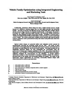
well-placement problem using coupled simulation-optimization approach for improved reservoir development [35-37]. The purpose of the implemented simulator, Eclipse 100, is specifying the objective function value at a selected well location. The optimizer tries to use the simulator as an objective function evaluator to find the coordination of the optimum well (i.e., Xw, Yw, coordinates of the well) and/or simultaneously finding the best completion layers (Zw1, Zw2). All codes are developed in MATLAB. As it is demonstrated in Fig. 1, our proposed approach starts by executing a command, which allows the reservoir simulator to be run in the MATLAB domain. The optimization process launches the simulator by passing a selected well location to its data file. At the next stage and after generating the results by the simulator, the code tries to search for the required data to calculate the objective function in the generated ASCII output file of the simulator. Fig. 1 shows the details of these communications between our developed code in MATLAB and the implemented commercial simulator, Eclipse 100.

tion constants, c1 and c2 (Eq. 1) each devoted to local or global best solutions. The velocity equation is described by weighting the acceleration constants using random numbers. Each potential solution flights towards the best location in the search space (Eq.1). In the following equation, inertia (W) is another criterion, which plays a pivotal role to explore the global optima. The more generated inertia values, the higher performance of the PSO convergence behavior is expected. The velocity of a particle X i is given as follows where rand1 and rand2 are random numbers between 0 and 1. These equations was a special case of investigations conducted by Eberhart and Kennedy [44]. Vi1  wVi  c1  rand1  (pBesti  X i )  c2  rand2  (gBesti  X i )

(1)

After achieving the potential solution, the new location of particles is updated based on the best previous solution and a new velocity, X i  X i  Vi 1 1

(2)

2.2. Implemented optimization algorithms

Start

Two different heuristic approaches have been selected as optimization tools, PSO and ABC. Both these methods are considered as heuristic methods [38-43]

Initializing Optimizer Algorithm

2.2.1. Particle swarm optimization Particle swarm intelligence was introduced by Eberhart and Kennedy [44]. Its terminology is based on the foraging behavior of the swarm of birds. Each optimal solution is found by a random population generation ( i {1, 2,..., n} , n is a number of populations) in the search space, which is being updated in each iteration. The potential solutions are generated by the initial location, Xi, and velocity, Vi, of particles before the beginning of each iteration. Each particle keeps track of the coordinates in the problem space by following the best value of two parameters, ‘pBest’ and ‘gBest’. ‘pBest’ is the currently feasible solution of the particle achieved so far, which is considered as the best solution (i.e., fitness). The optimum location of each particle, which is obtained by the global best location of PSO, is called ‘gBest’. At each step, the new velocity is calculated based on other two properties that are known as accelera-

Simulator Inputs (grid size, properties, PVT, SCAL data, etc.)

Collecting required data from Simulator Output

Calling Simulator at a new well location (X, Y, Z)

Calculating Objective Function (NPV) Yes

Check Optimum Criteria

NO

Figure 1. Workflow of the implemented optimal well placement algorithm. During well placement and/or completion optimization the same workflow is implemented.

39

R. Khoshneshin and S. Sadeghnejad / Journal of Chemical and Petroleum Engineering, 52 (1), June 2018 / 35-47

In this study, a robust and improved version of PSO known as modified PSO has been applied which is suggested by Zheng et al. [45] and Hu et al. [46]. In the modified PSO approach, a variable known as z k is defined as randomized descending inertia weight which has a great importance when it is applied to the inertia term and it presented as follows: the performance of PSO algorithm has been investigated by descending randomized equation. Z k is a matrix- vector expression and is given in Eq.3. Z k is a randomized term. A is a determinant of matrices of w and  .

1 and 2 are interval which confined to (0.5, 2).

P and p g are the best previous position of the i

th

particle and best particle position in current system in the k th iteration. Subsequent equations based on Zheng et al. study are provided below, Z k 1  AgZ k  1 gp  2 gpg (3) Z k  4  (rand)  (1  rand) w  0.5  (Zk )  0.5  (rand)

(4)

(5)

2.2.2. Artificial Bee Colony (ABC) ABC is another evolutionary optimization algorithm attributed to Karaboga [47], which was introduced based on the proposed model of Tereshko and Loengarov [48]. This algorithm shares a common characteristic with PSO, but its terminology is based on searching for rich food sources by honeybee colonies, in which onlookers, scouts, and employed bees are the key drivers in this nature-based algorithm. Some control parameters, which need to be defined to initiate this algorithm, are indicated in Table 1. Table 1. Description of control parameters in ABC algorithm. Parameter NP

Food Number=NP/2 Max cycle D

Description Colony size; sum of employed bees and onlookers Equals the half of the colony The number of cycles for foraging The number of parameters to be optimized

Employed bees locate the available food source. These bees follow onlookers that look into the

availability of food. When the food source is abandoned, employed bees act as scout bees and start to search for new food sources. This is one of the most remarkable characteristics of applying ABC. The potential solution is food number (Table 1). The position of employed bees is being updated if the new coordination is better than the former position. In Eq. 6 vij , xij , and xkj are the

new, current position of employed bees, and a random position of each bee, respectively. j is a randomly chosen parameter and k is a randomly chosen solution. Employed bees try to find neighbor food sources by using Eq. 6 which , in which ij represents a random number between 0 and

1. The equation below was suggested by Karaboga [47]. (6) vij  xij  ij  ( xij  xkj )

2.2.3. Objective function As it was mentioned in Fig. 1, subsequent to the generation of simulation data, the objective function should be evaluated by our developed code. Among copious objective functions, recovery factor, net present value (NPV), and maximum oil production are much of interests in the petroleum literature [7, 16, 37, 49-54]. Among these functions, since NPV attributes to capital revenues and expenditures is of particular interest [55, 56]. NPV is the differences between total revenue (e.g., oil production) and capital expenditure (e.g., excess water and gas treatment costs) over the period of a field life. Achieving maximum NPV during each scenario is the main goal. Thus, the NPV method can help us to decide the best optimization scenario among available ones. NPV function includes various variables as follow: Q repreP

sents as production value of phase P, C p is the revenue of producer wells that is related to phase P. n is equal to the period of simulation time (T) and Cd is an equation which calculates drilling

cost of a given well. The parameters of NPV function implemented in our study are presented in Table 2. T  Qo    1  Q   f g n    n 1 1  i  Q  w n  Y



Co      Cg    Cd    Cw  

(7)

40

R. Khoshneshin and S. Sadeghnejad / Journal of Chemical and Petroleum Engineering, 52 (1), June 2018 / 35-47

Cd  Nwell  Ltotal  Cd

(8)

Optimization Strategies

Table 2. Economic Parameters used during calculation of NPV function. Item Oil price (USD/bbl) Gas price (USD/MSCF) Discount factor (%) Excess water treatment costs (USD/bbl) Drilling costs (USD/ft)

Parameter Co Cg i

Value 40 2 15

Cd

800

Cw

0.5

Well Locating (completing in all layers)

Exploration Scenario

Well Locating with optimum completion

Exploration Scenario

Exploration Scenario

Infill Drilling Scenario

2.3. Optimization strategies and scenarios

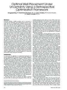
In our study, two different optimization strategies applied on two different scenarios (Fig. 2). Both optimization algorithms were examined in all cases. Fig. 3 depicts a schematic of all strategies and scenarios considered. The first strategy is well locating with full penetration completion in the formation under study (W#S1 in Fig. 3). In this optimization strategy, wells are completed in all layers of the formation irrespective of the amount of production of each layer. The second optimization strategy is searching for both optimum well location and optimum completion (W#S2 in Fig. 3), i.e., the optimum layers for completion. Due to production from a combination of high and low permeable layers, it is imperative to locate the ideal completion, which would increase actual production and limit the excess water and gas treatment costs. Two different scenarios namely exploration and infill drilling phase were considered in each optimization strategy. In the exploration phase scenario (Fig. 3a), our algorithm looks for the best location of a vertical wildcat well (i.e., an exploration well). In the other considered scenario, known as infill drilling (Fig. 3b), the main purpose is to keep producing from 9 available wells and to find the optimum location of the new well. Infill drilling as an effective solution applies when large numbers of wells are drilled to raise flow rate production in mature fields. Table 3. Reservoir Properties of the field under study. Parameter OOIP (STB) K* (md) Average Gross Thickness (ft) * (%) Initial reservoir pressure (psi) * represented as an average quantity.

Value 5.35 × 108 2186.37 280 18 3500

ABC

PSO

ABC

PSO

ABC

PSO

ABC

PSO

Figure 2. Optimization strategies and scenarios considered in this study for optimum well locating and optimum completion.

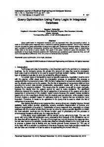
Figure 3. Schematic of two scenarios, a) exploration b) infill drilling scenarios. In both figures, W#S1 is an output schematic of an optimization strategy in which the location of the well with full penetration in the formation is considered. W#S2 shows the result of an optimization strategy wherein both location of the new well and its optimum completion are investigated.

2.4. Description of case study The case study in which the optimization process has been carried out is a 3-D black oil model with the block centered grid system. The case study used is from one of the Iranian offshore fields, which is dominated by a distributive fluvial system. The excellent reservoir sands of this field consist mainly of valley-fill deposition, where fluvial, coarse-grained sediment (with Darcy quality) accumulated in the upper and middle reaches of the incised valley system, while tidallyinfluenced sediments accumulated in the marineinfluenced middle and lower reaches (Estuary). As a result of this aggradation, less fluvial-derived sediment reached the lower reaches of the valley system. Fig. 4 shows the permeability map of this

R. Khoshneshin and S. Sadeghnejad / Journal of Chemical and Petroleum Engineering, 52 (1), June 2018 / 35-47

reservoir. Determining the optimum well placement in this heterogeneous reservoir is a tough decision due to its geological complexity. A sector of the formation was selected for well-placement optimization that consists of 36  60  7 grids. The field has °API of 20. Table 3 summarizes the average properties of the reservoir. Moreover, the histogram of permeability is depicted in Fig. 5. As shown in this figure, the reservoir contains a diverse range of permeability from 0 to 12000 md.

Figure 4. Permeability map of the field under the study. The fluvial geological system of the field is clear from this permeability map.

41

3.1. Well locating with full penetration during exploration scenario The optimization algorithms were simultaneously applied to optimize well spatial coordination. The well control of the wildcat well was held fixed at the flow rate of 3000 bbl/day. The optimizer tries to find the optimum well position across the formation area considering the physical boundary of the given field. Total production time of about 70 years was considered. Each optimization algorithm based on its methodology searches for the optimum condition and to compare them together 50 iterations (i.e., function calls) was considered during optimizations. Fig.6 compares the performances of ABC and modified PSO algorithms. The superiority of modified PSO to ABC in locating the optimal wild cat location is perfectly visible in Fig. 6. Although the NPV value calculated by PSO is slightly larger than that in ABC. PSO proves that based on its methodology, which is characterized by location and velocity of the best solution it is more robust than ABC at least in this case. Due to the ABC methodology that looks after the best food source, it could be able to find the optimum well location. The optimum location of the well was obtained at the grid cell of I=21 and J= 40 as shown in Fig. 7.

Figure 5. Distribution of permeability of the reservoir under study in md.

3. Results and Discussion In this section, the mentioned optimization strategies in Fig. 2, was implemented on the case study dataset. In addition, we compared the NPV from both optimization algorithms (i.e., ABC and PSO) of all optimization strategies (i.e., well placement and well located with optimum completion determination) during both scenarios (i.e., exploration and infill drilling).

Figure 6. Net present value versus number of simulation runs during PSO and ABC optimization in well locating with full penetration.

3.2. Well locating with full penetration during infill drilling scenario In this case, which is known as the infill drilling scenario, the field was producing with nine previously drilled wells. In the previous studies, a few

42

R. Khoshneshin and S. Sadeghnejad / Journal of Chemical and Petroleum Engineering, 52 (1), June 2018 / 35-47

number of wells in a synthetic model were examined [19, 50], while in this study, more wells at a larger scale on a real case study were analyzed.

The main difference of this case with the previous section is that the target is locating the 10th optimum well location after about 3700 days production with 9 available wells. The oil production continues until the field recovery be constant. Total production time, in this case, is about 47 years. All wells were producing with constant flow rate control with 900 bbl/day. More producer wells bring more complexities; therefore, implementing a robust and efficient algorithm can facilitate the optimization process. According to Fig.7, the highest NPV value for infill drilling phase was 1.80 1010 USD, which was achieved by the ABC algorithm. The recovery factor which is obtained by this algorithm is about 11.8% (Table. 4). The location of the new well and all previous nine wells are depicted in Fig. 8. The optimum well was found to be at I=9 and J=25. During the infill drilling, it is expected to locate wells in the formation where its oil has not produced yet (e.g., southeast of the formation and far from other wells) to increase sweep efficiency. Nevertheless, the location of this optimum well was considered near the previously drilled wells. Fig. 9 illustrates the location of this well, which is drilled just at the junction of two high permeable channels. This is why this location was considered as an optimum location as the more producible oil is recovered; the higher NPV value is expected.

Figure 7. Permeability map of the formation showing the optimal location of the wild cat during the exploration scenario. The well location was optimized by PSO algorithm.

Figure 8. Illustration of optimum location of the new well (determined by an arrow) during infill drilling scenario on oil saturation map. Before infill drilling phase, 9 wells were under production.

3.3. Locating well and finding optimum completion during exploration scenario In this strategy, unlike the former approach, the number of optimization parameters increases to four (i.e., I, J, K1, and K2). In the previous section, only the location of the well that was completed in all formation layers was considered (i.e., I, J). The production rates, duration, and well control parameters were considered as the previous strategy.

As it can be seen from Fig. 10, PSO is more efficient than ABC, which resulted in the NPV value of about 1.95 1010 USD. The optimal variables were obtained as: [7; 32; 4; 7]. It means that the optimum well location is at the grid of I=7 and J=32. In addition, the well should be completed from the 4th to the 7th layer. The length of the optimal completion is about 280 feet. There are two reasons for completing from the 4th layer and not from the shallower ones. First, as Fig. 11 shows, the 4th layer of the formation consists of a high permeable layer. Completing a well in this layer can result in higher production and consequently higher recovery factor. Moreover, due to the formation of a secondary gas cap during the infill drilling scenario, gas can breakthrough in shallower completions. Thus, not completing the well in those layers can decrease gas breakthrough in the production wells.

R. Khoshneshin and S. Sadeghnejad / Journal of Chemical and Petroleum Engineering, 52 (1), June 2018 / 35-47

43

3.4. Locating well and finding optimum completion during infill-drilling scenario Subsequent to the well locating in the exploration scenario, the infill-drilling scenario needs to be evaluated. All initial condition, as well as wellcontrol modes, were similar to the infill drilling in the first optimization strategy.

Figure 9. Arial view of the fluvial channels in the 4th layer of the formation which naturally causes to produce more oil.

Figure 10. Optimization advancement during optimum completion strategy for both PSO and ABC algorithms.

As shown in Table 4 and Table 5, the total field production rates are compared by applying two optimization strategies. It is evident that while the field productions costs i.e., total gas production and overall water production increase, the oil production will be decreased. Consequently, the NPV value becomes less and less. The ABC algorithm was capable of finding the best solution with the NPV value of 2.04 1010 USD. The optimum well was obtained at the location of I=30 and J=8 and completion layer of 3. Additionally, recovery factor and total field oil production were 13.05% and 7.88 104 bbl/day, respectively. The recovery factor of both strategies specifically infill drilling scenario has been shown in Table 5. Discrepancies drastically starts when optimum completion strategy has been applied. According to this figure, ABC clearly outperformed PSO in terms of recovery factor increasing. The reason behind this rising is that the best places which are abundant with probable oil production that has not been produced yet can be easily located by implementing ABC. As can be seen from Table 5 ABC can increase the recovery factor of about 8% greater than the PSO method using optimum completion strategy and 3.8% using full penetration strategy. It is evident that the infill drilling scenario has a great influence on increasing the production performance. Fig. 12 depicts the optimum location of the well. As it is clear, the well location is selected far from previously drilled wells to increase the sweep efficiency during production. In this situation, the intact oil can be produced and the recovery factor increases.

Figure 11. Map of permeability of the 4th layer of the reservoir under study showing by an arrow. The optimum location of the exploration phase has been determined across a channel and the optimum completion was selected in a layer (i.e., 4th layer) in which the channel is located.

The overall calculation time for ABC algorithm was 147 minutes for the same number of iterations; whereas PSO operative time was 180 minutes which it took quite longer than ABC algorithm elapsed time for infill drilling scenario. The simulations were run on a Core i7® 3.2 GHz CPU.

44

R. Khoshneshin and S. Sadeghnejad / Journal of Chemical and Petroleum Engineering, 52 (1), June 2018 / 35-47

the first strategy are well spatial coordinations while model parameters of the other scenario all are the same as first one except that the best layer which completed into reservoir formations. After performing several numerical simulations, the results and analyses of those two evolutionary algorithm are summarized as follows:

Figure 12. Optimum location of well (showing by an arrow) during infill drilling scenario on the oil saturation map. The optimum location of the well has been determined where its oil has not been produced yet.

4. Conclusion In this study, a general well placement optimization problem was investigated by utilizing two evolutionary algorithms to locate and place optimal well placement. Optimization parameters of

In infill drilling scenario, Overall calculation time for ABC algorithm was much more than PSO algorithm. Among all investigated scenarios and optimization strategies, ABC was more successful to achieve better results for locating optimum completion, and location during infill drilling scenario. Otherwise, modified PSO gained the better results in case of full penetration strategy specifically over the exploration scenario. As mentioned earlier, the x and y location of a well of the reservoir block were assumed to be variable, and depth parameter was assumed to be constant over the full penetration strategy. It was evident that high permeable layers of the reservoir are best decision to locate optimal well due to more oil which can be extracted from them.

Infill drilling scenario and specifically optimum, completion strategy has great importance since it can contribute to producing more probable and untapped oil from the reservoir.

Table 4. Comparison between the results of the full penetration strategy calculated by both algorithms.

Optimizer and Well Number ABC 1 Well PSO 1 Well ABC 10 wells PSO 10 Wells

NPV ($)

FOE (%)

1.94E+10 1.95E+10 1.80E+10 1.73E+10

12.91% 12.91% 11.78% 11.35%

FGPT (USD/MSCF) 4.92E+04 4.21E+04 6.36E+04 6.39E+04

FOPT (USD/bbl) 7.73E+04 7.73E+04 7.12E+04 6.86E+04

FWPT (USD/bbl) 1.73E+05 1.74E+05 1.64E+05 1.45E+05

Table 5. Results of total production obtaining by optimum completion strategy using both algorithms.

Optimizer and Number ABC 1 well PSO 1 well ABC 10 wells PSO 10 wells

Well

NPV ($) 1.99E+10 1.99E+10 2.04E+10 1.86E+10

FOE (%) 12.97% 12.91% 13.05% 12.10%

FGPT (USD/MSCF) 6.32E+04 2.10E+04 6.31E+04 6.33E+04

FOPT (USD/bbl) 7.83E+04 7.73E+04 7.88E+04 7.31E+04

FWPT (USD/bbl) 1.82E+05 1.13E+05 1.64E+05 1.70E+05

R. Khoshneshin and S. Sadeghnejad / Journal of Chemical and Petroleum Engineering, 52 (1), June 2018 / 35-47

References [1] Pan, Y. (1995). Application of Least Squares and Kriging in Multivariate Optimizations of Field Development Scheduling and Well Placement Design, Stanford University.

[2] Knudsen, B.R. and Foss, B. (2013). "Shut-in based production optimization of shale-gas systems." Computers & Chemical Engineering. Vol. 58, pp. 54-67. [3] Tavallali, M., Karimi, I., Teo, K., Baxendale, D. and Ayatollahi, S. (2013). "Optimal producer well placement and production planning in an oil reservoir." Computers & Chemical Engineering. Vol. 55, pp. 109-125.

[4] Shakhsi-Niaei, M., Iranmanesh, S.H. and Torabi, S.A. (2014). "Optimal planning of oil and gas development projects considering long-term production and transmission." Computers & Chemical Engineering. Vol. 65, pp. 67-80. [5] Brouwer, D. and Jansen, J. (2002). "Dynamic optimization of water flooding with smart wells using optimal control theory." in European Petroleum Conference, Society of Petroleum Engineers. [6] Sarma, P., Durlofsky, L.J., Aziz, K. and Chen, W.H. (2006). "Efficient real-time reservoir management using adjoint-based optimal control and model updating." Computational Geosciences. Vol. 10, No. 1, pp. 3-36.

[7] Zandvliet, M., Handels, M., van Essen, G., Brouwer, R. and Jansen, J.-D. (2008). "Adjointbased well-placement optimization under production constraints." SPE Journal. Vol. 13, No. 04, pp. 392-399. [8] Wang, C., Li, G. and Reynolds, A.C. (2009). "Production optimization in closed-loop reservoir management." SPE journal. Vol. 14, No. 03, pp. 506-523.

[9] Zhou, K., Hou, J., Zhang, X., Du, Q., Kang, X. and Jiang, S. (2013). "Optimal control of polymer flooding based on simultaneous perturbation stochastic approximation method guided by finite difference gradient." Computers & Chemical Engineering. Vol. 55, pp. 40-49.

[10] Volkov, O. and Voskov, D. (2016). "Effect of time stepping strategy on adjoint-based production optimization." Computational Geosciences. Vol. 20, No. 3, pp. 707-722.

45

[11] Yeten, B., Durlofsky, L.J. and Aziz, K. (2002). "Optimization of nonconventional well type, location and trajectory." in SPE annual technical conference and exhibition. Society of Petroleum Engineers. [12] Matott, L.S. (2006). Application of heuristic optimization to groundwater management. State University of New York at Buffalo.

[13] Wang, C., Li, G, and Reynolds, A.C. (2007). "Optimal well placement for production optimization." in Eastern Regional Meeting. Society of Petroleum Engineers. [14] Onwunalu, J.E. and Durlofsky, L. (2011). "A new well-pattern-optimization procedure for large-scale field development." SPE Journal. Vol. 16, No. 3, pp. 594-607.

[15] Wang, H., Echeverría-Ciaurri, D., Durlofsky, L. and Cominelli, A. (2012). "Optimal well placement under uncertainty using a retrospective optimization framework." SPE Journal. Vol. 17, No. 1, pp. 112-121.

[16] Bouzarkouna, Z., Ding, D.Y. and Auger, A. (2013). "Partially separated metamodels with evolution strategies for well-placement optimization." SPE Journal. Vol. 18, No. 06, pp. 1003-1011. [17] Forouzanfar, F., Poquioma, W.E. and Reynolds, A.C. (2015). "A covariance matrix adaptation algorithm for simultaneous estimation of optimal placement and control of production and water injection wells." in SPE Reservoir Simulation Symposium. Society of Petroleum Engineers.

[18] Jesmani, M., Bellout, M.C., Hanea, R. and Foss, B. (2016). "Well placement optimization subject to realistic field development constraints." Computational Geosciences. Vol. 20, No. 6, pp. 11851209.

[19] Al Dossary, M.A. and Nasrabadi, H. (2016). "Well placement optimization using imperialist competitive algorithm." Journal of Petroleum Science and Engineering. Vol. 147, pp. 237-248.

[20] Nozohour-leilabady, B. and Fazelabdolabadi, B. (2016). "On the application of artificial bee colony (ABC) algorithm for optimization of well placements in fractured reservoirs; efficiency comparison with the particle swarm optimization (PSO) methodology." Petroleum. Vol. 2, No. 1, pp. 79-89. [21] Rodrigues, H. W. L, Prata, B. A., and Bonates,

46

R. Khoshneshin and S. Sadeghnejad / Journal of Chemical and Petroleum Engineering, 52 (1), June 2018 / 35-47

T. O. (2016). "Integrated optimization model for location and sizing of offshore platforms and location of oil wells." Journal of Petroleum Science and Engineering. Vol. 145, pp. 734-741.

[31] Zhang, Y., Lu, R., Forouzanfar, F. and Reynolds, A.C. (2017). "Well placement and control optimization for WAG/SAG processes using ensemblebased method." Computers & Chemical Engineering. Vol. 101, pp. 193-209.

[23] Wang, X., Haynes, R. D., and Feng, Q. (2016). "A multilevel coordinate search algorithm for well placement, control and joint optimization." Computers & Chemical Engineering. Vol. 95, pp. 75-96.

[33] Nwachukwu, A., Jeong, H., Pyrcz, M. and Lake, L.W. (2018). "Fast evaluation of well placements in heterogeneous reservoir models using machine learning." Journal of Petroleum Science and Engineering. Vol. 163, pp. 463-475.

[22] Arnold, D., Demyanov, V., Christie, M., Bakay, A., and Gopa, K. (2016). "Optimisation of decision making under uncertainty throughout field lifetime: A fractured reservoir example." Computers & Geosciences. Vol. 95, pp. 123-139.

[24] Shirangi, M.G., Volkov, O., and Durlofsky, L.J. (2017). "Joint Optimization of Economic Project Life and Well Controls." in SPE Reservoir Simulation Conference. Society of Petroleum Engineers. [25] Lu, R., Forouzanfar, F., and Reynolds, A. (2017). "Bi-Objective Optimization of Well Placement and Controls Using StoSAG." in SPE Reservoir Simulation Conference. Society of Petroleum Engineers.

[26] Ramirez, B., Joosten, G., Kaleta, M., and Gelderblom, P. (2017). "Model-Based Well Location Optimization–A Robust Approach." in SPE Reservoir Simulation Conference. Society of Petroleum Engineers.

[27] Thimmisetty, C., Tsilifis, P., and Ghanem, R. (2017). "Homogeneous chaos basis adaptation for design optimization under uncertainty: Application to the oil well placement problem." AI EDAM. Vol. 31, No. 3, pp. 265-276.

[28] Montazeri, M. and Sadeghnejad, S. (2017). "An Investigation of Optimum Miscible Gas Flooding Scenario: A Case Study of an Iranian Carbonates Formation." Iranian Journal of Oil & Gas Science and Technology. Vol. 6, No. 3, pp. 4154. [29] Javaheri, P. and Sadeghnejad, S. (2017). "Effect of Injection Pattern Arrangements on Formation Connectivity During Water Flooding." in SPE Europec featured at 79th EAGE Conference and Exhibition. Society of Petroleum Engineers. [30] Sadeghnejad, S. and Masihi, M. (2017). "Analysis of a more realistic well representation during secondary recovery in 3-D continuum models." Computational Geosciences. Vol. 21, No. 5, pp. 1035-1048.

[32] Ghanem, R., Soize, C. and Thimmisetty, C. (2018). "Optimal well-placement using probabilistic learning." Data-Enabled Discovery and Applications. Vol. 2, No. 1, pp. 4-20.

[34] Rahmanifard, H. and Plaksina, T. (2018). "Application of fast analytical approach and AI optimization techniques to hydraulic fracture stage placement in shale gas reservoirs." Journal of Natural Gas Science and Engineering. Vol. 52, pp. 367-378.

[35] El Ouahed, A.K., Tiab, D. and Mazouzi, A. (2005). Application of artificial intelligence to characterize naturally fractured zones in Hassi Messaoud Oil Field, Algeria. Journal of Petroleum Science and Engineering. Vol. 49, No. 3, pp. 122141.

[36] Humphries, T.D., Haynes, R.D. and James, L.A. (2014). "Simultaneous and sequential approaches to joint optimization of well placement and control." Computational Geosciences. Vol, No. 18, No. 3, pp. 433-448.

[37] Li, L. and Jafarpour, B. (2012). "A variablecontrol well placement optimization for improved reservoir development." Computational Geosciences. Vol. 16, No. 4, pp. 871-889.

[38] Karaboga, D. and Basturk, B. (2007). "A powerful and efficient algorithm for numerical function optimization: artificial bee colony (ABC) algorithm." Journal of global optimization. Vol. 39, No. 3, pp. 459-471.

[39] Poli, R., Kennedy, J., and Blackwell, T. (2007). "Particle swarm optimization." Swarm intelligence. Vol. 1, No, 1, pp. 33-57.

[40] Karaboga, D. and Basturk, B. (2008). "On the performance of artificial bee colony (ABC) algorithm." Applied soft computing. Vol. 8, No. 1, pp. 687-697. [41] Karaboga, D. and Ozturk, C. (2011). "A novel

R. Khoshneshin and S. Sadeghnejad / Journal of Chemical and Petroleum Engineering, 52 (1), June 2018 / 35-47

clustering approach: Artificial Bee Colony (ABC) algorithm." Applied soft computing. Vol. 11 No. 1, pp. 652-657.

[42] Kennedy, J.,(2011) "Particle swarm optimization.." in Encyclopedia of machine learning, Springer. p. 760-766. Springer US.

[43] Civicioglu, P. and Besdok, E. (2013). "A conceptual comparison of the Cuckoo-search, particle swarm optimization, differential evolution and artificial bee colony algorithms." Artificial intelligence review. Vol. 39, No. 4, pp. 315-346.

[44] Eberhart, R. and Kennedy, J. (1995). "A new optimizer using particle swarm theory." in Micro Machine and Human Science, 1995. MHS'95., Proceedings of the Sixth International Symposium on, pp. 39-43 IEEE.

[45] Zheng, Y. L., Ma, L. H., Zhang, L.Y. and Qian, J. X. (2003). "Empirical study of particle swarm optimizer with an increasing inertia weight." in Evolutionary Computation, 2003. CEC'03. The 2003 Congress on, Vol. 2003, pp, 221-226. IEEE.

[46] Hu, X., Eberhart, R. C. and Shi, Y. (2003). "Engineering optimization with particle swarm." in Swarm Intelligence Symposium, 2003. SIS'03. Proceedings of the 2003 IEEE. pp. 53-57, IEEE. [47] Karaboga, D. (2005). "An idea based on honey bee swarm for numerical optimization." (Vol. 200). Technical report-tr06, Erciyes university, engineering faculty, computer engineering department.

[48] Tereshko, V. and Loengarov, A. (2005). "Collective decision making in honey-bee foraging dynamics." Computing and Information Systems. Vol. 9, No. 3, pp. 1-7.

[49] Beckner, B. and Song, X. (1995). "Field development planning using simulated annealingoptimal economic well scheduling and placeme-

47

nt." in SPE annual technical conference and exhibition. Society of Petroleum Engineers.

[50] Badru, O. (2003). Well-placement optimization using the quality map approach, Report, Department of Petroleum Engineering, Stanford University.

[51] Sarma, P., Aziz, K. and Durlofsky, L.J. (2005). "Implementation of adjoint solution for optimal control of smart wells." in SPE Reservoir Simulation Symposium. Society of Petroleum Engineers.

[52] Bangerth, W., Klie, H., Wheeler, M., Stoffa, P. and Sen, M. (2006). "On optimization algorithms for the reservoir oil well placement problem." Computational Geosciences. Vol. 10, No. 3, pp. 303319.

[53] Afshari, S., Aminshahidy, B., and Pishvaie, M.R. (2011). "Application of an improved harmony search algorithm in well placement optimization using streamline simulation." Journal of Petroleum Science and Engineering. Vol. 78, No. 3, pp. 664-678. [54] Shirangi, M.G. and Durlofsky, L.J. (2015). "Closed-loop field development under uncertainty by use of optimization with sample validation." SPE Journal. Vol. 20, No. 5, pp. 908-922.

[55] Bukhamsin, A.Y., Farshi, M.M. and Aziz, K. (2010). "Optimization of multilateral well design and location in a real field using a continuous genetic algorithm." in SPE/DGS Saudi Arabia Section Technical Symposium and Exhibition, Society of Petroleum Engineers.

[56] Pajonk, O., Schulze-riegert, R., Krosche, M., Hassan, M. and Nwakile, M.M. (2011). "Ensemblebased water flooding optimization applied to mature fields." in SPE Middle East Oil and Gas Show and Conference. Society of Petroleum Engineers.