VLSI Placement and Area Optimization Using a Genetic Algorithm to ...

VLSI Placement and Area Optimization Using a Genetic Algorithm to Breed Normalized Postfix Expressions Christine L. Valenzuela (Mumford)∗and Pearl Y. Wang† Published in 2002

Abstract

ily produce duplications and deletions of the basic rectangles when applied to the binary tree representation and may create illegal expressions if applied to postfix representations. These difficulties can be overcome. This paper describes a solution approach that incorporates a novel encoding system with a simple and effective GA. It utilizes an order-based representation that encodes the rectangles and the binary operations into a simple permutation of structures, and a decoder that converts the permutation of structures into a normalized postfix expression. The normalized postfix expression is a non-redundant representation because it produces a unique postfix representation for every distinct slicing floorplan. If the postfix expressions are not constrained by normalization, a single layout can be expressed by very many equivalent postfix expressions. (Details of normalized postfix expressions are given in section 2 of this paper.) VLSI floorplanning is an important stage in chip design. It involves the placement of a set of rectangular circuit modules (macro cells) on a chip so as to minimize the total area and the total interconnecting wire length. When placing macro cells, many of the circuit modules are themselves not yet fully designed and frequently have some flexibility in their shape. For example, a circuit module made up from 12 identical components may have them placed in one row of 12 components, 2 rows of 6 components, 3 rows of 4 components, etc., offering the floorplan designer a range of possible shapes for that module. Circuit modules having flexibility in their shape are often referred to as soft modules, and those with no flexibility in their shape are called hard modules. Using a technique based on a slicing floorplan, which can be obtained by recursively dividing a rectangle into two parts with either a vertical or a horizontal cut, it is possible to fully exploit the available flexibility of soft modules and efficiently combine module placement and area optimization into a single algorithm. An alternative to the slicing floorplan is the non-slicing floorplan, in which there is no require-

We present a genetic algorithm (GA) that uses a slicing tree construction process for the placement and area optimization of soft modules in very large scale integration floorplan design. We have overcome the serious representational problems usually associated with encoding slicing floorplans into GAs, and have obtained excellent (often optimal) results for module sets with up to 100 rectangles. The slicing tree construction process used by our GA to generate the floorplans has a run-time scaling of O(n lg n). This compares very favourably with other recent approaches based on non-slicing floorplans that require much longer run times. We demonstrate that our GA outperforms a simulated annealing implementation with the same representation and mutation operators as the GA. Keywords: Floorplanning, genetic algorithm, normalized postfix expression, simulated annealing, slicing tree.

1

Introduction

Simulated annealing (SA) and tabu search (TS) tend to be more popular than genetic algorithms (GAs) with crossover for solving large combinatorial problems. One reason for this is the difficulty involved in devising representations for GAs that facilitate effective crossover operators. The very large scale integration (VLSI) floorplanning problem provides a particularly challenging application. The candidate floorplan solutions are frequently represented either as binary trees or as postfix expressions, both of which encode specific instructions for combining the rectangles in pairs using a mix of symbols to represent the basic rectangles and binary operators. Naive GA crossover operators eas∗ Christine Valenzuela (Mumford) is with the School of Computer Science & Informatics, Cardiff University, CF24 3AA, UK. † Pearl Y. Wang is with the Department of Computer Science, George Mason University, Fairfax, VA 22030-4444 USA.

1

ment for recursive construction, and tighter packings may be possible using this approach. Stockmeyer [14] examined cases where each subcircuit may have different layout alternatives in a floorplan and showed that there is an efficient polynomialtime area optimization algorithm for slicing floorplans, whereas the area optimization problem for non-slicing floorplans is NP-Hard. The main disadvantage of the slicing floorplan approach is that for a particular set of circuit modules, the majority of the feasible layouts will be non-slicing [9]. In other words, the slicing floorplan approach severely reduces the size of the search space and may eliminate the very best circuit layouts. On the other hand, reduction in the size of the search space is advantageous as long as the solutions are good enough. According to [20] this is indeed the case for problems where modules have flexibility in their shape. Another feature of the slicing floorplan that makes it an attractive proposition is the simple way that solutions can be represented as normalized postfix expressions [19]. It is interesting to note that techniques involving soft modules and slicing floorplans are equally applicable to facility layout problems [4, 5] as they are to VLSI floorplanning. Non-slicing floorplan design for VLSI is often dealt with by separating the two stages of placement and area optimization, and many researchers in recent years have concentrated extensively on the area optimization stage [11, 12, 18]. A recent nonslicing placement technique called the sequencepair method [8] has been extended to handle soft modules and area optimization [7]. However, the sequence-pair method has to solve expensive convex programming problems in order to determine the exact shape of each module and this results in a very long run time. Another relatively new technique called the bounded sliceline grid (BSG) packing algorithm [9] has proved successful in the placement of hard rectangles, i.e., rectangles that have no flexibility in their shape. The BSG approach is very adaptable and is able to accommodate modules that are not rectangular and modules which are allowed to partially overlap. On the downside, though, a single application of the BSG packing algorithm scales at T (n) = O(n2 ) for hard modules given the n x n grid size suggested by the authors. This compares with T(n) = O(n) for hard modules using a slicing floorplan approach. The average case run time scaling of the combined placement and area optimization algorithm of slicing floorplans for soft modules is T (n) = O(n lg n). It would appear that we are the first to use encoded normalized postfix expressions in our GA. Although several other examples of GAs applied

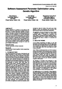
to slicing tree structures can be found in the literature, they do not use normalized expressions. Schnecke and Vornberger [13], for example, used a GA to manipulate the slicing tree directly for VLSI floorplanning problems. However the crossover involves complex repair mechanisms simply to ensure that the final product (or offspring) represents a legal slicing floorplan, with no duplications or deletions of modules. Cohoon et al. [2], in what is probably the best known study of its type, used a collection of four different crossovers and applied them to postfix expressions that were not normalized. In a more recent study Kado et al. [5] compared the approach of Cohoon et al. with some other techniques from the literature and also some new approaches, based on seeding the initial population. Kado et al. were able to improve on published results for several facility layout problems using a variety of non-normalized representations and further improvements have since been made to some of these results by Garces-Perez et al. [4] using Genetic Programming . Kr¨oger [3], working on two-dimensional bin packing problems, also used non-normalized postfix expressions and devised a crossover that searches the parental expressions for subtrees that do not have any rectangles in common, and combines subtrees from both parents into the offspring. Although Kr¨oger’s GA outperformed his SA algorithm, the processing involved with the crossover he used was both complex and time consuming. We view our main contribution to the field of slicing tree optimization as the extension of the ideas of [19] which used a normalized postfix representation for SA. Through the addition of an encoding system, we have adapted the approach to produce a simple but effective GA. We test our GA on soft modules from the benchmark MCNC data sets, ami33, ami49, and playout and also on a larger data set that we independently generated. The objective of our present study is a ‘proof of concept’ and we limit our objective function to the construction of a floorplan of minimum area. Other elements, such as the minimization of the total wire length, will be included in the cost function at a later date. To complement our GA, we have written some supporting software that checks the final floorplan for correctness and draws a picture of the layout. Figure 1 shows the roles played by the different software components. The process by which the GA evaluates individual postfix expressions is complicated when soft modules are involved. Each time a pair of rectangles or subassemblies is combined, a range of possibilities is stored for heights and widths. At the end of the construction process the best floorplan (i.e., the one with the smallest 2

Figure 1: Schematic showing the relationships between the software and data components of the system. In Section 4 we outline our GA and explain the order based genetic operators we have used. Section 5 describes our simulated annealing implementation and Section 6 defines the data sets we have used. Section 7 presents our results and, finally, we provide a summary of our achievements and outline our plans for future work in Section 8. The present paper expands the work presented in [16].

percent dead space) is chosen from a range of candidate solutions. The backtrack program receives the postfix expression from the GA and re-evaluates the floorplan (i.e postfix string) using the same procedure as the original GA, only this time vital intermediate stages are saved. Once the postfix expression has been evaluated and the dimensions of the enclosing rectangle established, the backtrack program traces through the saved intermediate stages, retrieving the exact heights and widths of all the component rectangles. In addition to its vital role in calculating dimensions for the basic rectangles as input to the drawing tool, the backtrack program carries out several verification procedures. First, it checks that all the modules are present in the final floorplan. Second, it checks that the module dimensions are correct given their areas and shape flexibilities. Finally it verifies the percentage of dead space produced by the GA. The backtrack program terminates when it has finished all its checking and established the precise dimensions of the basic modules and stored all of these in a file. It is this file, now a file of hard modules, that provides the data for the drawing tool. The drawing tool produces a diagram of a floorplan by re-evaluating the postfix expression, backtracking this time to establish relative placement positions for all the basic modules in the floorplan.

2

Slicing Structures and Postfix Representations

A slicing floorplan is a rectangular floorplan with n basic rectangles that can be obtained by recursively cutting a rectangle into smaller rectangles using a series of vertical and horizontal edge-to-edge (i.e., guillotine) cuts. A slicing floorplan can be represented in the form of a binary tree, called a slicing tree, in which each internal node of the tree is labelled either * or +, corresponding to a vertical or a horizontal cut respectively. Each leaf represents a basic rectangle and is labelled between 1 and n, where n is the total number of basic rectangles. A slicing tree can be represented, alternatively, using a postfix expression. The postfix expression is derived by carrying out a post-order traversal. There is a one-to-many relationship between slicSection 2 begins with a review of slicing floor- ing floorplans and slicing tree representations for plans and their postfix representations, and then slicing floorplans. If we restrict our representations describes our approach to shape-curve addition for to skewed slicing trees, however, we obtain unique the combination of soft modules. Section 3 de- depictions for slicing floorplans [19]. The postfix exscribes the representation used to encode our slicing pression derived from a skewed slicing tree is called floorplans and also the decoder, which interprets a normalized postfix expression, and provides a linthese structures as normalized postfix expressions. ear form of the representation. Figure 2 (a) il3

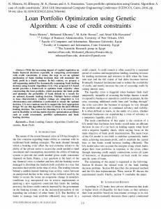
Figure 3: Binary operations for slicing floorplans.

We deal with the two main components of the floorplanning process separately in the two subsections that follow. Figure 2: Slicing floorplan (a), skewed slicing tree representation of floorplan (b) and corresponding normalized postfix expression (c).

A. The Placement Stage and the Binary ‘+’ and ‘*’ Operations In the discussion so far, we have viewed a slicing tree as a top-down description of a slicing floorplan in which the slicing tree specifies how a given rectangle is cut into smaller rectangles by vertical and horizontal cuts. An alternative is to view a slicing tree as a description of a bottom-up procedure. From a bottom up point of view the slicing tree describes how pairs of rectangles can be combined recursively to yield larger rectangles. Figure 3 shows the actions of the binary operations + and * on the two rectangles A and B: ‘+’ puts B on top of A, and ‘*’ puts B on the right of A. In the example depicted in Figure 3, the two rectangles A and B combine under + and * to form L-shaped modules. When following a bottom up slicing tree description however, each L-shaped module (and any other shaped modules which are not rectangular) will be replaced by the smallest possible enclosing rectangle, resulting in the creation of dead space (or waste) in the floorplan. Determining exactly where to position each rectangle is frequently referred to as the placement problem, and is NP-Hard. A simple lower bound for a brute-force algorithm that searches the solution space of normalized postfix expressions can be obtained if we make a simplifying assumption that places a single operator between each pair of operands in the expression, from the second to the nth on the postfix list, (i.e., either a ‘*’ or ‘+’), giving 2n−1 choices for the whole postfix string. Thus, considering the n! orderings of the rectangles and the choices for the operators, a lower bound on the total number of distinct postfix strings is 2n n! giving the following lower bound for the run time complexity of the brute-force algorithm

lustrates a typical slicing floorplan, (b) shows the skewed slicing tree, and (c) the normalized postfix expression representing the floorplan in (a). A skewed slicing tree is a slicing tree in which no node and its right child have the same label in { *, + } and it is obtained by making consecutive vertical cuts from right to left, and making consecutive horizontal cuts from top to bottom. A normalized postfix expression is obtained by traversing a skewed slicing tree in post-order and is characterized by chains of {*, + } operators in which the operators alternate. For example, the postfix expression 1 2 3 + * 4 * is normalized, but the expression 1 2 3 + + 4 * is not (because of the two adjacent + symbols). A slicing floorplan with n-1 cuts will produce n basic rectangles. Thus a postfix expression consists of exactly 2n - 1 entries. A normalized postfix expression which characterizes a slicing floorplan can be written: π1 c1 π2 c2 π3 c3 π4 c4 ,.......,πn cn where π1 π2 π3 π4 .......πn represent a permutation of the 1,2,...,n basic rectangles, and the ci ’s are chains of operators, either + * + * + *...., or * + * + * ...... (see [19] for more details). If we let P l(ci ) represent the length of the chain, ci , then i l(ci ) = n - 1, and l( c1 ) = 0. Also the maximum length of any chain of operators, ci , is constrained by the balloting property as follows: for any position, i : 1 ≤ i ≤ n, l(ci ) ≤ i - 1. For slicing floorplans, postfix expressions provide a convenient mechanism with which to represent various placements alternatives. The process of floorplan design requires a further stage, however, when soft modules are involved – area optimization. 4

T (n) = Ω(2n n!n), assuming that it takes a time of Θ(n) to process each individual string. In order to derive a simple upper bound for a similar brute-force algorithm, we examine all the individual possibilities for the operator chains lying between each pair of operands in a normalized postfix expression. The length of the operator chain is zero following the first rectangle, but from the second rectangle in the list onwards the length of the chain following the ith rectangle can take any integral value from the set { 0, 1, 2,..., (i-1) }. Furthermore, an operator chain of any given non-zero length can exist in one of two possible forms: either * + * + * ... or + * + * +.... Following the second operand in the postfix expression, for example, the possibilities for operator chains are either no operators (i.e., the empty chain), or a single operator selected from {*, + }, giving three possibilities. Following the third operand are five possible chains: the empty chain, *, +, * + or + *. Following the ith operand are 2*(i-1) + 1 possible operator chains; however the total number of operators for the entire postfix string is constrained to n - 1. A simple upper bound can be obtained by considering the n! orderings of rectangles, together with the above mentioned 2*(i-1) + 1 possible operator chains following the ith operand. Once again we assume that it takes Θ(n) time to process each string. T(n) ≤ Cn!*(1 * 3 * 5 *.....*(2*(i-1) + 1) *.....* (2*(n-1) + 1)n < Cn!*(2 * 4 * 6 * * 2i * .... * 2n)n = Cn!2n n!n where C is a positive constant, giving the simple upper bound O(n!n!2n n) (Note: our upper bound and lower bound differ by a factor of n!.) For problems such as these, where very large search spaces are involved, meta-heuristics, such as GAs may provide the only viable options.

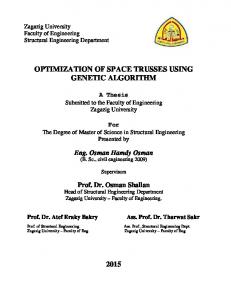
Figure 4: Shape curve for a module with shape flexibility 3.

For the purposes of our present study we adopt the definition of shape flexibility from [20] as it provides a continuous range of candidate aspect ratios for our soft modules. For a soft module with aspect ratio, ρ, such that 1/r ≤ρ ≤ r, various vertical (y coordinate) and horizontal (x coordinate) dimensions are possible and these can be modelled by a shape curve, Γ. Γ is a continuous non-increasing curve lying entirely within the first quadrant, such that the x and y coordinates of points lying on or above the curve define the feasible region. Figure 4 illustrates a typical shape curve for a rectangle of area 3 and shape flexibility 3. The two points on the curve mark the limits of flexibility for the rectangle, which means that the rectangle can only be made taller or wider than 3 units if dead space is added. The feasible region depicted in the diagram indicates possible height and width dimensions for an enclosing rectangle and covers all points on and above the curve. Pairs of soft modules, A and B, can be combined into super modules by adding their shape curves: A B +, by adding along the y direction and A B *, by adding along the x direction. Figure 5 and Figure 6 illustrate examples of the vertical (+) and horizontal (*) combinations of pairs of modules. When a pair of soft modules is combined, the new shape curve can be computed simply by adding the curves at the points which correspond with the so-called ‘corners’ on the curves of the component modules. The diagrams show clearly that the shape curves for basic modules of fixed orientation (i.e. no rotation is allowed) are each completely characterized by two ‘corners’. (Note: a hard module of fixed orientation is characterized

B. Area Optimization Using Soft Modules Flexible circuit modules or soft modules are characterized by their aspect ratios. Let a given rectangle, R, have height h(R), width w(R), and area A(R). The aspect ratio of R is the ratio h(R)/w(R). A soft rectangle is one that can have different shapes as long as the area remains the same. The shape flexibility of a soft rectangle specifies the range of its aspect ratio. A soft rectangle of area A(R) is said to have a shape flexibility r if and only if R can be represented by any rectangle of area A(R) for which: 1 r

≤

h(R) w(R)

≤r 5

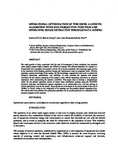
Figure 6: Adding shape curves for A B *. Shape flexibility of A is 2 and B, 3.

Figure 5: Adding shape curves for A B +. Shape flexibility • Case 2: One module has a ‘corner’ at this position, and the width position lies between two corners on the curve for the other module.

for A is 2 and for B, 3.

completely by a single point or ‘corner’.) Figure 5 illustrates the addition of two shape curves for a vertical combination, where module B is placed on top of module A to produce a new enclosing rectangle, C. The shapes curves for modules A and B each consist of two ‘corners’, A[1] and A[2] for modules A and B[1] and B[2] for module B. A[1] and B[1] define the minimum widths for A and B, and A[2] and B[2] define their maximum widths. The parts of the curves laying between the minimum and maximum widths for A and B give all the possible height and width combinations for area(A) = 2 and area(B) = 3. The minimum width of the enclosing rectangle for the vertical combination of any two modules X and Y can never be narrower than the larger of the two minimum widths,X[1] or Y [1], and so if X[1] 6= Y [1] the smaller is discarded in calculating the shape curve for combined module. In Figure 5, however, A[1] = B[1] , thus no points are discarded. The maximum width of the new enclosing rectangle C is the same as the larger of the two maximum widths (B is this case). Dead space is added to the narrower module (A) to make C into the required rectangular shape. When adding together two shape curves in a vertical direction we only add at positions corresponding to ‘corners’ on one or other of the component shape curves. We identify three cases which can occur when adding such pairs of points at a given width position:

• Case 3: One module has a ‘corner’ at this position, and the width position lies beyond the last corner for the other module.

The ‘corners’, C[1], C[2], and C[3], for the combined module, C, in Figure 5 illustrate cases 1, 2 and 3 respectively, and can be obtained as follows: Case 1 C[1].width = A[1].width (=B[1].width) C[1].height = A[1].height + B[1].height Case 2 C[2].width = A[2].width C[2].height = A[2].height + Area(B)/A[2].width Case 3 C[3].width = B[2].width C[3].height = B[2].height + A[2].height Note that the shape curve addition process shown in Figure 6 for horizontal combination can be obtained in the same way as for Figure 5 by simply reversing the heights and the widths. In order to produce a slicing floorplan from a normalized postfix expression it is necessary to create a repetitive process that combines modules that result from previous combinations (called super modules) with a mix of basic modules and other super modules, adding together their shape curves in the bottom-up procedure. Fortunately, the process of adding shape curves for super modules is essentially the same as the procedure for combining two basic modules, only with more ‘corners’ to add. Our • Case 1: Both component modules have ‘cor- general calculation routines for adding points on ners’ at this width position, pairs of shape curves extend the ideas illustrated 6

in Figure 5. The details are based on the following observation:

lists are simple to maintain; the one sorted on x coordinates is the exact reverse of the list sorted on y coordinates. This has important run-time consequences: no sorting algorithm is needed to update either of the lists. As described above, a basic module of fixed orientation has a maximum of two ‘corners’. Thus, when two basic modules are combined by our methods the resulting combined module will have at most four ‘corners’ on its shape curve. After combining n modules following an arbitrary slicing tree, an upper bound on the number of points is 2n. Currently the run time for our shape curve combination routine is rather long because we have not as yet incorporated approximations as suggested in [19] to reduce the number of ‘corners’ accumulated by our shape curves. The worst case run-time for our routine, assuming that one module is added at a time to a single super module, (e.g., the postfix expression1 2 + 3 + 4 + 5 + 6 +) is given by:

• For any given shape curve, the area between two consecutive ‘corners’, either along the width or along the height axis, varies in a uniform fashion. Thus if point Z lies half way between ‘corners’ X and Y along, say, the width axis, the area at point Z will lie half way between the areas at X and Y . This simple relationship holds because each ‘corner’ on a curve, except for the first, represents the maximum width (height) possible for one of the basic modules contained within the curve. Thus between any two ‘corners’, dead space is added at a uniform rate This simple observation makes it easy to calculate heights and widths exactly for any position on a given shape curve, whether or not that position corresponds to a ‘corner’ and no matter how many basic modules have been included to produce the shape curve. The pseudocode of the main routine for vertical combination is presented in Algorithm 1. Details for the three alternative methods of combination, case 1, case 2, and case 3, referred to in the algorithm, are as described earlier in the present section. For each basic module and super module the ‘corners’ are stored in a simple list of coordinate pairs sorted on increasing value of the x (or width) coordinate. In addition to the height and width values, a third variable is stored with each coordinate pair: the amount of dead space. The list of coordinate pairs represents the ‘corners’ of the shape curve for a module. The algorithm proceeds by stepping through a pair of lists (one list for each of the modules to be combined) in ascending sequence of x coordinates value, adding the two curves together as it proceeds, producing a new list for the resulting combined module. As explained the ‘corner’ selected as a starting point for the addition process is the earliest point on the module with the larger of the minimum x values as its first ‘corner’. Any ‘corners’ from the other module with x values smaller than this minimum are discarded. The routine for horizontal combination is obtained by interchanging the x and the y coordinates in the code and working through simple lists of shape curve points, this time sorted on ascending y value. To facilitate both vertical and horizontal combinations, we maintain two sorted lists of coordinates for each module and super module: one sorted on ascending x values, and the other on ascending y values. If redundant points (i.e., points that lie in the feasible region but above the shape curve) are eliminated as soon as they are generated, the two

T (n) = O(n2 ). The best and the average case, however, are given by: T (n) = O(n lg n) [14]

3

The Representation and Decoder

Our representation for the GA is order based and consists of an array of records, with one record for each of the basic rectangles of the data set. Each record contains three fields: • a rectangle ID field : this identifies one of the rectangles from the set {1, 2, 3,..., n} • an op-type flag: this boolean flag distinguishes two types of normalized postfix chains, T = + * + * + * +...., and F = * + * + * + *..... • a chain length field : this field specifies the maximum length of the operator chain associated with the rectangle identified in the ID field. Our decoder converts a given instantiation of the array of records into a legal normalized postfix expression by writing down the rectangle IDs in the order given, and inserting the type of normalized chain of operators (either T = + * +... or F = * + *...) as indicated by the op-type flag associated with that rectangle ID. The length of each chain of operators is given in the chain length field. For 7

Figure 7: Algorithm 1. Add shape curves algorithm. Main routine for the vertical combination of two soft modules. Details for Cases 1, 2, and 3 combinations are given.

8

The GA breeds permutations of records from which our decoder produces normalized postfix expressions. These expressions are, in turn, processed by adding the shape curves together (as described in Section 2) for each horizontal or vertical combination, recording the percent of dead space at the end. The initial population consists of random permutations of records with each basic rectangle represented exactly once in each list. The op-type flag for each record is set to ‘+’ or ‘*’ with equal probability, and the value in the length field is generated in two stages: Stage 1: length = 0, with a probability of 0.5 Stage 2: if the length is not set to zero, then it is generated from a Poisson distribution with mean 3.

example, for a length = 5 we would get an operator chain of either + * + * + or * + * + * , depending on the value of the op-type flag. However, if a chain of operators produced in this way turns out to be too long and violates the balloting property (i.e. if we are currently processing the ith rectangle in the list the total number of operators in the postfix expression constructed so far must be less than or equal to i - 1), the decoder will shorten the chain and maintain legality. If the decoder reaches the end of the sequence of records and the resulting postfix string has less than n 1 operators, extra operators are added on to the end of the string maintaining the normalized pattern of ..+ * + *... etc. The decoder algorithm is presented in Algorithm 2. Below is an example showing an encoded string and its normalized postfix interpretation: rect5 op-type* length 2

rect2 op-type+ length 1

rect4 op-type* length 0

rect1 op-type* length 2

rect3 op-type+ length 0

A. Genetic Operators for Permutations

Postfix expression generated: 5 2 + 4 1 * + 3 +

4

We use three different mutation operators, one for each of the fields in our encoding structure (rectangle ID, op-type, and op length):

The Genetic Algorithm

• M1 Swap positions of two rectangle IDs. Our GA, presented in Algorithm 3 is an example of a steady state GA based on the classification given in [15]. It also uses the weaker parent replacement strategy first described in [1]. As outlined in Algorithm 3, our GA applies genetic operators to permutations of rectangle records. The fitness values are based on the amount of dead space produced in each floorplan, F , defined by the individual normalized postfix expressions encoded in the population. The percentage of dead space is defined as follows: A(RF )−

Pn

Pn i=1

i=1

A(Ri )

A(Ri )

• M2 Invert op-type flag, + to * or vice versa. • M3 Mutate length by incrementing or decrementing (i.e. length = length + 1, length = length - 1) with equal probability. (If length is zero we always increment). M1 and M2 produce an identical effect to the M1 and M2 operators defined in [19]. Our M3 operator, on the other hand, is different from theirs, although its effect is similar. But M3 will never produce an illegal postfix string. In the very early stages of our study we chose some non-problem specific position-based and order-based crossovers for testing and carried out some extensive tests to compare the performance of four permutation crossovers on our data sets. Overall cycle crossover (CX) [10] came out best. Our implementation of CX is efficient and runs in linear time.

× 100

where A(RF ) is the area of the enclosing rectangle for the floorplan and A(Ri ) is the area of the ith basic rectangle. In Algorithm 3 the first parent is selected deterministically in sequence, but the second parent is selected in a roulette wheel fashion, the selection probabilities for each genotype being calculated using the following formula:

5

(Rank) selection probability = P Ranks

Our Simulated Annealing Implementation

Our simulated annealing implementation is similar to that which is described in [19]. It is based on the routine developed in [6]. A generic simulated annealing procedure is outlined in Algorithm 4. In the outer loop the temperature is reduced gradually. At

where the genotypes are ranked according to the values of the waste that they have produced, with the worst ranked 1, the second worst 2, etc., and the best ranked highest. 9

Figure 8: Algorithm 2. Outline decoder algorithm.

Figure 9: Algorithm 3. Simple steady-state GA.

Figure 10: Algorithm 4. Generic SA.

10

each step of the inner loop a small perturbation, S 0 , of the configuration, S, is chosen and the resulting change in the cost function, ∆ = C(S 0 ) − C(S), is computed. The new configuration is accepted with probability 1 if ∆ ≤0, and with probability e−∆/T if ∆ > 0. The higher the temperature, the more likely it is that a poorer solution than S is accepted. We use the same representation and decoder for our SA as for our GA. The perturbations are selected from M1, M2, and M3, the mutations from the genetic algorithm in the previous section, with one of the three moves selected at random each time. M1 and M3 are each selected with 40% probability, whilst M2 (which is more disruptive) is selected with 20% probability, the same proportion as we use in our GA. As we previously mentioned, our M1 and M2 are identical with the M1 and M2 operators used in [19], and M3 produces a similar effect to the M3 used in their work. We use a temperature schedule of the form Tk = r*Tk−1 , k = 1, 2, 3, .... and set r = 0.9. The initial temperature, T0 is determined by computing a sequence of random moves, using M1, M2, and M3, and computing the quantity ∆avg, the average value of the magnitude of change in cost per move. We should have e∆/T = P '1, for T = T0 , so that there is a reasonable probability of acceptance at high temperatures. We start with a temperature of 2.5*∆avg , which equates to P '0.7. The starting parameters r and P , were set following extensive experimentation. At each temperature we attempt 20n moves (inner while loop), following [21, 22]. 20n is also the size of the population we use for our GA. The annealing process is halted when the temperature has been lowered 20 times since the last improvement was recorded in the best-so-far (outer while loop). Experimentation indicates that the SA is unlikely to produce any further improvements at this stage. In our implementation M3, which increments or decrements the length of a selected normalized operator chain, frequently produces perturbed solutions that result in floorplans identical to their precursor. This happens because our decoder ‘corrects’ information in the operator ‘chain length’ field whenever it contradicts the balloting property, by adding or subtracting operators where required. Thus we find that quite a large number of moves involving no change in cost are produced throughout the execution of the SA, and all such moves are accepted in our implementation. Nevertheless it would appear that these ‘sideways’ moves are beneficial to the SA process overall, introducing variability which may lie dormant for a period and yet can be expressed physically at a later time, following further M3 mutations at different locations in the 11

postfix expression: if we prevent our SA from accepting moves where no change in cost is involved, our results deteriorate considerably. We find that it can be beneficial if we refocus the SA search, from time to time, onto the global best floorplan so far discovered. We do this whenever three consecutive temperature reductions have failed to produce any improvements to the global best.

6

The Data Sets

We use the basic modules of the MCNC benchmarks ami33, ami49, and playout, and model the shape flexibility as continuous curves in a manner similar to [21, 22]. An additional problem, f 100, was randomly generated following the guidelines of [19]. The areas of the modules for f 100 were chosen from a uniform distribution of floating point numbers between 1 and 20. Details for the individual data sets are given in Table 1.

7

Results

In this section we compare the performance our GA and the related SA on a range of problems consisting of between 33 and 100 soft modules. It is unfortunate that despite using modules taken from the three larger MCNC benchmark problems, ami33, ami49, and playout, we are unable to make direct comparisons with published results in [21, 22, 23], because of the extra constraints on that have been imposed by these authors on selected modules in each data set. For example, in [21] 2 - 4 of the modules are pre-placed in fixed positions, and in [22] 1 -5 of the modules are restricted to the chip boundary. In [23] the authors mix hard and soft modules, allowing no flexibility in the shapes of 2 - 5 of the modules in each data set. Although at the start of [21] and [22] the authors outline some rather more straightforward experiments on ami33 and ami49, and report results of less than 1 % dead space, no details of shape flexibility are given. Additionally, an estimate of wire length is included in their objective function, although this is not quoted in their results, which is stated only in terms of percentage dead space. We will discuss these points further in the following section, after we have presented our results. As we have mentioned, we choose a population size of 20n for our GA where n is the number of modules in the problem. The GA is halted when 40 generations have passed since the last improvement was recorded in the best-so-far, as it seems to have converged by then.

For the GA and SA, we set the limits on the aspect ratio for the final enclosing rectangle (i.e. the chip aspect ratio) to those used in [19]: 1/2 ≤ chip aspect ratio ≤ 2. Unfortunately, there does not appear to be a way to predict a chip aspect ratio in advance of a full evaluation of a postfix expression. To ensure that we obtain acceptable solutions, we automatically reject all moves for the SA and offspring for the GA in which the best point on the final shape curve does not correspond to a legal chip aspect ratio. Following rejection, crossover and mutation operators are reapplied at new random positions until an individual with a suitable aspect ratio is produced. In the rare event of 25 consecutive attempts failing to produce a suitable individual in the GA, one of the parents is replaced and the process attempted again. It is interesting to note that both the GA and the SA appear to favour floorplan solutions with chip aspect ratios close to the boundaries, and the production of neighbourhood solutions which lie outside of these boundaries are a frequent occurrence, especially for the SA. (When we removed the chip aspect ratio constraint, the results were even more extreme, producing only very long and skinny layouts.) The results for our GA and SA are summarized in Table 2. Where possible we have carried out 100 replicate GA or SA runs, each with different random starts, and averaged the results. The data sets in column 1 are as detailed in Section 6 of this paper. The value in brackets in column 1 gives the shape flexibility of the basic rectangles for the experiments in the row. Column 2 specifies the number of replicate runs used for averaging the GA and SA results in each row. We used 100 experiments for the smaller problems (ami33 and ami49 ), and less for the larger problems. Columns 3 and 6 summarize the dead space obtained by the GA., and columns 7 and 9 summarize the results for the SA. The average percentage of dead space of the best floorplan is recorded for the GA and SA in columns 3 and 7 respectively, and the overall best from the replicate runs is recorded in columns 6 and 9. The total number of postfix expression evaluations (including those individuals subsequently rejected because of illegal chip aspect ratios) averaged over all the replicate runs is noted in columns 4 and 8, and the average run times for the GA appear in columns 5. Run times for the GA were recorded on a Pentium III computer running at 600 MHz with 128 Mbyte RAM. Run times for our SA have not been included, but they are directly proportional to the total number of evaluations, and are thus similar to the run times for the GA. However, we note that, evaluation for evaluation, the SA has the potential to run very much faster than the GA because it is 12

better suited to storing and re-using partial floorplan results. We have, as yet, made no attempt to optimize our SA code, and our present implementation recomputes each newly generated neighbourhood floorplan in its entirety, in the same fashion as for the GA. The grey shaded cells in the table indicate situations where floorplans have been found that are known to be optimal (because they have zero percent dead space). The results presented in Table 2 indicate that the GA is better than the SA for the data sets under consideration. Statistical tests bear this out, showing significant differences between the GA and SA means for the ami33, ami49 and playout data sets at the 0.02 % level. It is clear, however, that relaxing the shape flexibility of the basic modules from 2 to 4 makes it easier for the both algorithms to find good floorplans. Throughout the study we found that the GA was much more robust and easier to tune than the SA: the SA producing much more variable and unpredictable results. The average performance of the SA on the three variants of the 100 module problem was particularly poor, and comparing the total number of evaluations for the SA with the GA for the 100 module problems, the SA appears to become trapped in a poor suboptimal region early on. Some caution is needed in interpreting the results for 100 modules, however, because we carried out only 5 replicate experiments in each case. Figure 13 and Figure 14 show typical floorplan designs found by our GA for ami33 and ami49 respectively. These pictures were constructed using our drawing tool, which is part of our supporting software described in the introduction to the present paper.

8

Conclusions Work

and

Further

This paper describes a GA that uses a novel encoding and a simple order-based approach to breed normalized postfix expressions for macro cell placement and area optimization in VLSI floorplan design. Our experiments confirm that simple orderbased genetic operators are effective in guiding the genetic search for floorplanning. Results presented for floorplanning problems with up to 100 modules frequently achieve optimal solutions: and this is something that we have not observed in related published work. Comparisons between our GA and a related simulated annealing (SA) implementation clearly demonstrate the superiority of the GA for solution quality and robustness.

Figure 11: Table 1 Characteristics of the data sets.

Figure 12: Table 2 Means of sets of replicate runs for % dead space for genetic algorithm and simulated annealing.

13

The only recent related work, of which we are aware, is that reported in [20, 21, 22, 23], which uses soft modules and normalized postfix expressions with a simulated annealing algorithm. In [20] experiments using test problems with 100 modules are briefly described in the introduction to the paper. Each module has a shape flexibility 2, and the SA yields, on average, 2.2 % dead space. Our result of 1.98 % on our 100 module data (shape flexibility 2) would appear to be very similar, although the other authors do not state whether or not any constraint is imposed upon the final aspect ratio for the chip (we constrain our solutions to chip aspect ratios between 1/2 and 2). In the introduction to another paper [22], results are reported of less than 1 % dead space for several MCNC benchmarks including ami33 and ami49. Once more it would appear that these results are very similar to ours: we mostly achieve zero percent dead space for the same problems. However, Young and Wong do not state the range of aspect ratios which they allow for the soft modules in their experiments. Although we are not yet able to match the runtimes reported in [20, 21, 22, 23], we expect to achieve a significant speedup when we introduce piecewise linear approximations and reduce the number of ‘corners’ we accumulate during the construction process. We currently perform exact calculations when adding our shape curves. Our plans include extensive experimental studies to assess the effect that reducing the maximum number of ‘corners’ that a shape curve is allowed to have on the accuracy of the dead space calculation. Our supporting software will provide all the verification and crosscheck tools that we require to carry out these studies. We have shown that our novel genetic representation for normalized postfix expressions can be applied successfully to slicing floorplans. Not only do our algorithms produce excellent results but the slicing tree construction process used by our GA to generate the floorplans has a run time scaling of O(n) for hard modules, and O(n lg n) for soft modules. This compares very favourably with the bounded-sliceline grid (BSG), that has been used in GAs and SA for VLSI placement in recent papers. The BSG packing algorithm scales at O(n2 ) for hard rectangles, given the n x n grid size suggested by the authors. Work in progress is currently focussed on floorplan design using soft modules with free orientation (as opposed to fixed orientation), and also on adapting some simple bin packing heuristics for floorplanning problems. We have recently succeeded in incorporating wire length into the objective function for our GA, and early experi-

Figure 13: Ami33 floorplan with shape flexibility 2, and dead space 0 %.

Figure 14: Ami49 floorplan with shape flexibility 2, and dead space 0 %.

14

ments have produced some promising results. The planned incorporation of shape curve approximations into our area optimization code has already been mentioned. In addition we have adapted our floorplanning techniques and applied them to some facility layout problems [17].

Acknowledgements We should like to thank the editor and the anonymous referees for their helpful comments and suggestions. We believe the paper has been much improved due to their insight.

[11] Peichen Pan and C. L. Liu, Area Minimization for Floorplans, IEEE Transactions on Computer Aided Design of Integrated Circuits and Systems, Vol. 14, No 1, January 1995., pages 123-132. [12] M. Rebaudengo and M. Sonza Reorda, Floorplan Area Optimization Using Genetic Algorithms, Proceedings of Fourth Great Lakes Symposium on VLSI, March 1994, pages 22-25. [13] V. Schnecke. and O. Vornberger, Genetic Design of VLSI-Layouts, the First International Conference in Genetic ALgorithms in Engineering Systems: Innovations and Applications (GALESIA), IEE 1995, pages 430-435. [14] L. Stockmeyer, Optimal Orientations of Cells in Slicing floorplan Designs, Information and Control, vol. 59, pages 91-101, 1983.

References [1] D. J. Cavicchio. Adaptive search using simulated evolution. Unpublished doctorial dissertation, University of Michigan, Ann Arbor, 1970. [2] J. P. Cohoon, S. U. Hedge, W. N. Martin and D. S. Richards. Distributed Genetic Algorithms for the Floorplan Design Problem. IEEE Transactions on Computer Aided Design, Vol. 10, No. 4, April 1991, pages. 483-492. [3] Berhold Kr¨ oger, Guillotineable bin packing: A genetic approach, European Journal of Operational Research 84, pp 645-661, 1995. [4] Jaime Garces-Perez, Dale A. Schoenefeld and Roger L. Wainwright, Solving Facility Layout Problems Using Genetic Programming. Proc. 1st Annual Conference in Genetic Programming, pages 182-190, 1996. [5] Kazuhiro Kado, Peter Ross and David Corne, A Study of Genetic Algorithm Hybrids for Facility Layout Problems. Proc. 6th International Conference on Genetic Algorithms, pages 498-505, 1995. [6] S. Kirkpatrick, C. D. Gelatt Jr. and M. P. Vecchi, Optimization by simulated annealing. Science (220), pages 671-680, 1983. [7] H. Murata and Ernest S. Kuh, Sequence-pair based placement method for hard/soft /pre-placed modules, International Symposium on Physical Design, pages 167-172, 1998. [8] S. Nakatake, H. Murata, K. Fujiyoushi. and Y. Kajitani. Rectangle-packing-based module placement. Proceedings IEEE International Conference on Computer-Aided Design, pages 143-145, 1995. [9] S. Nakatake, K. Fujiyoshi, H. Murata and Y. Kajitani. Module Placement on BSG-Structure and IC Layout Applications, Proceedings of ICCAD, pages 484-491, 1996 [10] I. M. Oliver, D. J. Smith, and J. R. C. Holland, A study of permutation crossover operators on the traveling salesman problem. Genetic Algorithms and their Applications: Proceedings of the Second International Conference on Genetic Algorithms, pages 224-230, 1987.

15

[15] G. Syswerda, Uniform Crossover in Genetic algorithms. Proceedings of the Third International Conference on Genetic Algorithms. Hillsdale, NJ: Lawrence Erlbaum Associates, 1989. [16] Christine L. Valenzuela, and Pearl Y. Wang. A Genetic Algorithm for VLSI Floorplanning. Parallel Problem Solving in Nature - PPSN VI. Lecture Notes in Computer Science 1917, pages 671-680 September 2000. [17] Christine L. Valenzuela, and Pearl Y. Wang. Breeding Normalized Postfix Expressions for the Facility Layout Problem. Fourth Metaheuristic International Conference (MIC 2001), Porto, Portugal, July 16-20, pages 261- 265, 2001. [18] Ting-Chi Wang and D. F. Wong, Optimal Floorplan Area Optimization, IEEE Transactions on Computer Aided Design. Vol. 11, No. 8, pages 9921002 August 1992. [19] D. F. Wong, H. W. Leong and C. L. Liu, Simulated Annealing for VLSI Design, Kluwer Academic Press, Boston MA, 1988. [20] F.Y. Young and D.F. Wong, How Good are Slicing floorplans, Integration, the VLSI Journal, Vol 23, pages 61-73, 1997. [21] F. Y. Young and D. F. Wong, Slicing floorplans with pre-placed modules. Proceedings IEEE International Conference on Computer-aided Design, pages 252-258, 1998. [22] F. Y. Young and D. F. Wong, Slicing floorplans with boundary constraints. IEEE Asia South Pacific Design Automation , pages 17-20, 1999. [23] F. Y. Young and D. F. Wong, Slicing floorplans with range constraints. International Symposium on Physical Design, pages 97-102, 1999.