Well Placement Optimization Using a Genetic Algorithm With ...

SPE 118808 Well Placement Optimization Using a Genetic Algorithm with Nonlinear Constraints Alexandre A. Emerick, SPE, Petrobras S.A., Eugênio Silva, Bruno Messer, Luciana F. Almeida, Dilza Szwarcman, Marco Aurélio C. Pacheco and Marley M.B.R. Vellasco, PUC-Rio

Copyright 2009, Society of Petroleum Engineers This paper was prepared for presentation at the 2009 SPE Reservoir Simulation Symposium held in The Woodlands, Texas, USA, 2–4 February 2009. This paper was selected for presentation by an SPE program committee following review of information contained in an abstract submitted by the author(s). Contents of the paper have not been reviewed by the Society of Petroleum Engineers and are subject to correction by the author(s). The material does not necessarily reflect any position of the Society of Petroleum Engineers, its officers, or members. Electronic reproduction, distribution, or storage of any part of this paper without the written consent of the Society of Petroleum Engineers is prohibited. Permission to reproduce in print is restricted to an abstract of not more than 300 words; illustrations may not be copied. The abstract must contain conspicuous acknowledgment of SPE copyright.

Abstract Well placement optimization is a very challenging problem due to the large number of decision variables involved and the nonlinearity of the reservoir response as well as of the well placement constraints. Over the years, a lot of research has been done on this problem, most of which using optimization routines coupled to reservoir simulation models. Despite all this research, there is still a lack of robust computer-aided optimization tools ready to be applied by asset teams in real field development projects. This paper describes the implementation of a tool, based on a Genetic Algorithm, for the simultaneous optimization of number, location and trajectory of producer and injector wells. The developed software is the result of a two-year project focused on a robust implementation of a computer-aided optimization tool to deal with realistic well placement problems with arbitrary well trajectories, complex model grids and linear and nonlinear constraints. The developed optimization tool uses a commercial reservoir simulator as the evaluation function without using proxies to substitute the full numerical model. Due to the large size of the problem, in some cases involving more than 100 decision variables, the optimization process may require thousands of reservoir simulations. Such a task has become feasible through a distributed computing environment running multiple simulations at the same time. The implementation uses a technique called Genocop III – Genetic Algorithm for Numerical Optimization of Constrained Problems – to deal with well placement constraints. Such constraints include grid size, maximum length of wells, minimum distance between wells, inactive grid cells and user-defined regions of the model, with non-uniform shape, where the optimization routine is not supposed to place wells. The optimization process was applied to three full-field reservoir models based on real cases. It increased the net present values and the oil recovery factors obtained by well placement scenarios previously proposed by reservoir engineers. The process was also applied to a synthetic case, based on outcrop data, to analyze the impact of using reservoir quality maps to generate an initial well placement scenario for the optimization routine without using an engineer-defined configuration. Introduction The definition of a well placement is a key aspect with major impact in a field development project. In this sense, the use of reservoir simulation allows the engineer to evaluate different placement scenarios. However, the current industry practice is still, in most cases, a manual procedure of trial and error that requires a lot of experience and knowledge from the engineers involved in the project. Considering that, the development of well placement optimization tools which can automate this process is a high desirable goal. Well placement optimization is a very challenging problem due to the large number of decision variables involved and the nonlinearity of the reservoir response as well as of the well placement constraints. Over the years, a lot of research has been done on this problem, most of which using optimization routines coupled to reservoir simulation and economical models. In 1995, Beckner and Song1 applied a Simulated Annealing algorithm to optimize the location and scheduling of 12 wells with fixed orientation and length. In 1997, Bittencourt and Horner2 applied a Genetic Algorithm (GA) hybridized with Polytope and Tabu Search methods to optimize the location of 33 vertical and horizontal wells, including wells, producers and injectors. In 1998, Pan and Horner3 investigated the use of multivariate interpolation algorithms, Least Squares and Kriging, as proxies to reservoir simulations for optimization problems including well placement. In 1999, Cruz et al.4 introduced the concept of “quality map”, which is a two-dimensional representation of the reservoir responses. They suggested that quality

2

SPE 118808

maps could be a helpful tool for choosing well locations, with fewer full field simulation runs. In 2001, Montes et al.5 applied GA to optimize the location of vertical wells and analyzed the effects of internal parameters on the performance of the GA. In 2003, Yeten et al.6 proposed a methodology for the optimization of type, location and trajectory considering multilateral wells. Their methodology is based on a GA and includes hill climber, artificial neural network and near well scale up algorithms to accelerate the optimization. In the same year, Badru et al.7 applied a hybrid GA to optimize vertical and horizontal wells. In 2005, Ozdogan et al.8 proposed a methodology called Fixed Pattern Approach which uses a hybrid GA to locate wells on user-defined patterns. To our knowledge, they were the first to attempt on geometrical constraints of the well placement problem considering non-uniform shape of the reservoir. Recently, Handels et al.9, Wang et al.10 and Sarma and Chen11 proposed different approaches for well placement optimization using gradient-based optimization techniques. The application of gradient-based methods seems promising due to the efficiency of these methods in terms of number of simulation runs. However, there are some issues, such as possible discontinuities in the objective function and nonlinearities in well placement constraints, which make the application of gradient-based methods very difficult, especially to problems with arbitrary well trajectory in complex model grids. Most of the researches focused on the performance of the optimization process, trying to minimize the number of required simulation runs. However, the development of computer hardware and software has been changing the execution scenario of reservoir simulators. The use of clusters with a large number of CPUs currently allows several reservoir simulations to be executed at the same time, which makes the optimization process using the full numerical model as the evaluation function a feasible task. Furthermore, despite the large number of researches about well placement optimization, there is still a lack of robust computer-aided optimization tools ready to be applied by asset teams into real field development projects. This paper describes the implementation of a tool based on a Genetic Algorithm for the simultaneous optimization of number, location and trajectory for producer and injector wells. The developed software is the result of a two-year project focused on a robust implementation of a computer-aided optimization tool to deal with realistic well placement problems with arbitrary well trajectories, complex model grids and linear and nonlinear constraints. The developed optimization tool uses a commercial reservoir simulator as the evaluation function without using proxies to substitute the full numerical model. Due to the large size of the problem, in some cases involving more than 100 decision variables, the optimization process may require thousands of reservoir simulations. Such a task has become feasible through a distributed computing environment running multiple simulations at the same time. The implementation uses a technique called Genocop III – Genetic Algorithm for Numerical Optimization of Constrained Problems (Michalewicz and Nazhiyath12) – to deal with well placement constraints. Such constraints include grid size, maximum length of wells, minimum distance between wells, inactive grid cells and user-defined regions of the model, with non-uniform shape, where the optimization routine is not supposed to place wells. Background Genetic Algorithm Genetic Algorithm (GA) is a robust optimization technique based on analogies to natural selection and genetics. GA combines concepts such as survival of the fittest individual and random crossing information. The first application of GA to optimize a complex problem was presented by Holland13 (1975). In his work, he demonstrated the ability of bit chains to represent complex problems and that those chains can be improved by simple transformations. The modeling of a GA consists in codifying each possible solution of a problem on a structure denominated chromosome, which is composed by a chain of variables denominated genes. These chromosomes represent individuals. The search process for an optimal solution consists in the submission of a collection of individuals, or a population, to an evolutionary process that occurs in cycles. Each evolutionary cycle is called a generation and includes the following stages: evaluation, selection, crossover and mutation. During evaluation, a fitness value is associated to each individual, which quantifies how well the solution represented by that individual solves the problem, when compared to other individuals in the population. Based on the fitness values, on the selection stage, a group of individuals is elected for reproduction. The most fitted individuals, on a generation, have greater chances to be selected. Reproduction can be done by two different operators: crossover and mutation. The crossover operation combines genes from two individuals to generate new individuals as a mix of genes from the original individuals. The mutation operation is applied at selected individuals separately. The mutation operator sets a random value to a gene; this operation inserts new genetic information in the population. Hence, reproducing the natural processes of evolution, it is possible to assume that, after several generations of evolution, the population will have individuals with better fitness than the ones on the first generation. A special operator used in this work is the controlled mutation, which selects one individual and then operates only onto its wells’ positions genes. Instead of selecting a random value for a gene, like in a normal mutation operation, the well’s position is moved by exactly one grid block. As in Faletti14,15 and Túpac16 the evolution process starts with the creation of random individuals to form an initial population. The new individuals are inserted into the population, removing the less fitted individuals from the previews generation. The new population is then evaluated and the cycle (evaluation, evolution) is restarted. The stop condition for the cycling is a maximum number of generations.

SPE 118808

3

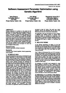
Genetic Algorithms for Constrained Problems Most of the methods proposed for handling nonlinear constraints in Genetic Algorithms for optimization problems are based on penalty functions. However, the performance of these methods is highly problem-dependent. Moreover, many methods require additional tuning of several parameters. In 1995, Michalewicz and Nazhiyath12 proposed an alternative method called Genocop III – Genetic Algorithm for Numerical Optimization of Constrained Problems – to deal with linear and nonlinear constraints. The Genocop III method uses two separate populations, but an evolution in one of them influences evaluations of individuals in the other one. The first one is called search population and consists of individuals which satisfy the linear constraints of the problem. The second population, called reference population, consists only of fully feasible individuals, i.e., individuals who satisfy all constraints (linear and nonlinear). The reference individuals are directly evaluated in the beginning of the optimization process and so are the feasible search individuals. However, unfeasible search individuals are "repaired" prior to the evaluation. This repairing process consists of the random selection of a reference individual (Ri) and the application of a crossover operator between the unfeasible search individual (Si) and Ri until a new feasible individual (Z) is found and then evaluated. Additionally, if the evaluation of Z is better than the evaluation of Ri, this individual replaces Ri in the reference population. Also, Z can replace Si with some probability pr. Figure 1 illustrates the Genocop III procedure.

S1

R1

S2

Z

R2 S4 R4 R3 Feasible region

S3

begin P = pr; // replacement probability if feasible(S) == false Z = aS + (1 – a)R; // a ∈ [0, 1] while feasible(Z) == false Z = aZ + (1 – a)R; // a ∈ [0, 1] end while if evaluation (Z) > evaluation(R) R = Z; end if if rand() ≤ P S = Z; // S is replaced by Z else evaluation(S) = evaluation(Z); end if end if end.

Ri – reference individuals Si – search individuals Figure 1 – Genocop III procedure.

Using this Genocop III procedure, it is possible to deal with the following well placement constraints in the optimization process: ƒ Grid size: I ij ∈ ⎡⎣1,I grid ⎤⎦ ; J ij ∈ ⎡⎣1,J grid ⎤⎦ and K ij ∈ ⎡⎣1,K grid ⎤⎦

( xi 2 − xi1 )

2

+ ( yi 2 − yi1 ) + ( zi 2 − zi1 ) ≤ Lw max 2

2

ƒ

Maximum length of wells:

ƒ

Minimum distance between wells: Dist ( welli ; well1..Nwell ) ≥ Dw min

ƒ

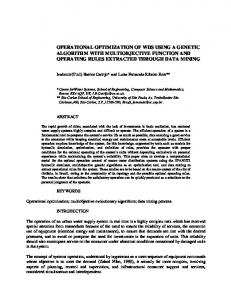
Inactive grid cells. In this case we have defined that a well cannot have the heel point and toe point in an inactive grid cell. However, a well may cross inactive cells (Figure 2).

ƒ

User-defined regions of the model, with non-uniform shape, where the optimization routine is not supposed to place wells. In this case, any part of the well may not cross this region (Figure 2).

With this set of constraints the optimization algorithm becomes applicable to reservoir models with non-uniform geometry. These constraints also allow some flexibility in the definition of the optimization problem. For instance, the engineer can define just a small region of the model and optimize the location of some infill drilling wells while keeping the minimum allowed distance to wells already drilled in the field.

4

SPE 118808

Inactive grid cell Unfeasible well Feasible well

Porosity 0.36

Unfeasible well Well-1

Well-2

Well-3

User-defined region without wells

0.08 I-J Section view

Well-1

I-K Section view

Figure 2 – Well placement constraints. In this figure, Well-1 crosses a region with inactive grid cells, but it is still a feasible well because the heel and toe points are inside active cells. Well-2 is an unfeasible well because it starts in an inactive grid cell. Well-3 is also an unfeasible well because it crosses an user-defined region where wells are not supposed to be placed (blue region in the figure).

Methodology Problem parameterization This work defines 8 decision variables to characterize each well: ƒ Three variables define the starting point (heel point) of the well (I, J and K coordinates). ƒ Three variables define the ending point (toe point) of the well (I, J and K coordinates). ƒ One binary variable define the well type: producer or injector. ƒ One binary variable define the well status: active or inactive. Due to this parameterization, with 8 decision variables per well, the optimization problem becomes large. For instance, considering a case with a maximum number of 15 wells, the problem will require 120 variables to be optimized. On the other hand, this parameterization allows the simultaneous optimization of well location, trajectory, type and, once the maximum number of wells is defined, the optimization of the number of active wells as well. Figure 3 shows a schematic representation of the chromosome used in the GA. A chromosome represents an individual of the population and each individual corresponds to a different well placement scenario. Well 1

I11

J11

K11

Heel point

I12

Well N

J12

K12

Toe point

T1

S1

...

IN1

JN1

KN1

Type Status

Figure 3 – Representation of the chromosome.

IN2

JN2

KN2

TN

SN

SPE 118808

5

The given parameterization also allows some flexibility in the definition of the optimization problem. For example, instead of optimizing all attributes (well’s location, trajectory, type and number), it is possible to optimize only some of them. For instance, one can optimize only the trajectory of the wells by optimizing the toe point and keeping constant all other decision variables. In this case, the problem will, in fact, be smaller, with only 3 decision variables per well (Figure 4). Actually, one can imagine several different optimization problems to be worked out, such as: to optimize only producers or only injectors, to optimize only a group of wells and keep constant the other wells, to optimize only the number of wells, etc.. Well 1

I11

J11

K11

Heel point constant

I12

J12

Well N

K12

T1

S1

...

IN1

JN1

KN1

IN2

JN2

KN2

TN

SN

Toe point Type Status constant To be optimized

(a) Initial case

(b) After trajectory optimization

Figure 4 – Optimization of only the trajectory of wells.

Definition of the Initial Population The definition of the initial population may impact on the performance of the optimization process. It is likely that a population of poor individuals will require several generations until it produces a good solution. In this sense, employing the engineer´s knowledge to set up the initial population is highly desirable. In the implementation being presented, two different approaches are taken to generate the initial population, depending on whether the engineer defines or not some initial well placement scenarios: Initial population with no engineer-defined well placement scenario In this case, the whole initial population is defined randomly, including the search population and the reference population (which satisfies all linear and nonlinear constraints). Tests made have shown that, in this case, it is necessary to increase the population size and number of generations in order to obtain good results. Initial population with engineer-defined well placement scenarios If the engineer defines some initial well placement scenarios, the following heuristic is used to generate the search population and the reference population: ƒ The engineer’s suggested scenarios will represent 10% of the initial search population and the other individuals will be generated randomly. ƒ The engineer’s suggested scenarios will represent 50% of the reference population and the other individuals will be generated randomly. With this approach there is a large probability that, after the optimization process, the final solution will be an offspring of the engineer’s cases. In fact, this is the aim of this approach. The idea is to search for solutions around the engineer’s suggested scenarios. It is likely that, if the engineer defines a good initial case, the final solution, obtained by the optimization process, will be an “improved engineer’s defined case” and probably will resemble the initial one. However, if the engineer’s defined case is not a good initial solution, it might influence negatively the performance of the optimization process. In these cases, probably the optimization would get better results by initializing the whole population randomly. Tests made to date have shown that, at least for more complex cases, using this approach will lead to better solutions than using the engineer’s defined cases just as single individuals of the search population and also better than starting the process with the whole population defined randomly.

6

SPE 118808

Limitations of Methodology Deterministic simulation-based optimization The optimization process is based on a deterministic realization of the simulation model. In fact, some authors17,18,19 have shown that the uncertainties have an important impact on the result of optimization. However, due to the large size of this optimization problem and the required computation cost of the implementation in question, it is not feasible to perform optimizations for a large number of reservoir realizations. This is a very important limitation of the given approach. In order to reduce this problem, it is suggested that, before the optimization, the engineer performs an uncertainty analysis with an initial well placement scenario to define a “most likely” or P50 model, and then performs the well placement optimization with this P50 model. After that, it is possible to perform another uncertainty analysis to evaluate the impact of the uncertainties on the result of the optimization. Depending on the results, the engineer can also define a new P50 model and perform another optimization and so on. Note that this approach is not different from the current practice on field development projects. Well scheduling The well placement optimization assumes that all wells start producing and injecting at the same time. There is no schedule optimization. Also, the production constraints, such as bottom-hole pressure and fluid production limits, are assumed to be constant during the simulation. Features of the Optimization Tool Well representation The well representation used in the optimization process makes no explicit distinction between vertical, horizontal or deviated wells. All wells are defined as a straight line in a 3D space. To accurately represent the well in the simulation model, a routine which identifies the grid cells crossed by each well and calculates the Cartesian coordinate of the entry point and exit point of the well in each cell was implemented. This information allows the calculation of the well indices using a feature of the reservoir simulator20. Distributed simulations Due to the large size of the problem, in some cases with more than 100 decision variables, the optimization process may require thousands of reservoir simulations. In order to deal with this large number of simulations, it was also developed, as part of this work, a system to distribute and manage the simulations in a computer cluster . This system is based on two types of XML Web services: the Distributor and the Executor. The Distributor receives from the optimization algorithm a description of the group of simulations to be executed and it takes care of allocating these simulations to several Executors. Net present value calculation The objective function of the optimization process is the net present value (NPV) of the field development project. So, a simplified NPV calculation, which considers the following parameters, was implemented: ƒ Oil and gas sale prices. ƒ Oil, gas and water production costs. ƒ Water injection cost. ƒ Production unit (platform) cost. ƒ Relative position among wells and the platform to calculate the total cost of risers and flow lines. ƒ Three different prices for wells, according to its deviation degree. ƒ Taxes and royalties. Production controls For each simulation, all wells are attached to the same production group. To that group, several production controls can be specified, such as maximum liquid and oil production rate, maximum water injection rate, void replacement control, etc. Adaptative genetic operator parameters Generally, a genetic algorithm will produce better results if the crossover and mutation rates are adaptative, that is, if they are dynamically adjusted as the evolution proceeds. Usually, the crossover rate should be high and the mutation rate low at the beginning of the evolution, which tends to make better use of the initial genetic material in the population without moving to randomly through the solution space. Accordingly, as the number of generations increase, the population tends to converge to a reduced variety of individuals and the mutation rate should be increased in order to favor the introduction of new genetic material. In this work, the crossover rate decreases and the mutation rate increases linearly, with the generations, from an initial given value to a final one.

SPE 118808

7

Applications Field 1 The first case study is an off-shore field in Campos Basin. The simulation model for this field has 83 × 45 × 23 grid cells (31,486 actives) and two wells with fixed location, one producer (P1) and one injector (I1). Based on this model, a reservoir engineer proposed a well placement scenario adding more 13 wells, 8 producers and 5 water injectors, using high deviated wells with a maximum length of 800 meters (Figure 5).

P1 I1

Inactive grid cells Figure 5 – Base case – Field 1. Producers are in black and water injectors in blue. Notice that this figure shows the projection of the wells in the first layer of the model. In fact, these wells are not necessarily completed in the same grid layer.

For this field, two optimizations were performed, the first one using the well placement scenario proposed by the engineer in the initial population of the GA, and the second one starting the whole population randomly. The maximum number of wells was set equal to 13, which corresponds to an optimization problem with 104 decision variables. Table 1 shows the GA parameters and Table 2 shows the well constraints used in both optimizations. Table 1: GA parameters – Field 1.

Table 2: Wells constraints – Field 1.

Population size Number of generations

Producer wells Maximum liquid rate Minimum bottom hole-pressure Maximum water-cut Water injector wells Maximum water rate Maximum bottom hole-pressure Maximum number of wells Maximum length of wells Minimum distance between wells

Steady state Crossover Mutation Controlled mutation

100 50 Initial 20% 65% 8% 5%

Final 5% 8% 30% 25%

1,800 m3std/d 180 kgf/cm2 0.95 (shut-in well) 3,000 m3std/d 350 kgf/cm2 13 800 m Non-constrained

Figures 6 and 7 show the evolution of the NPV during the optimizations. In these figures, the NPV of each simulation was normalized with respect to the NPV of the base case (well placement scenario proposed by the engineer). The first optimization performed 4,209 reservoir simulations and obtained an increase of 28% over the base case NPV; an increase of 13% was achieved in the cumulative oil production. The second optimization performed 4,893 reservoir simulations and obtained a NPV 20% higher than the base case value; a cumulative oil production 6.5% higher was attained. Table 3 summarizes the results and Figure 8 shows the production curves. Table 3: Optimization results – Field 1.

Case

Simulations

Base case Optimized 1 (from base case) Optimized 2 (no initial guess)

4,209 4,893

Producers 9 8 9

Wells Injectors 6 6 6

NPV 1.000 1.282 1.199

Cumulative Oil Production 1.000 1.130 1.065

8

SPE 118808

1.282

Normalized NPV

1.30

1.30

1.10

1.10

0.90

0.90

0.70

0.70

0.50

0.50

0.30

0.30

0.10

0.10 SIMULATIONS

-0.10

-0.10

BASE CASE FINAL BEST NPV

-0.30

-0.30

BEST NPV -0.50

-0.50 0

500

1000

1500

2000

2500

3000

3500

4000

Simulation number Figure 6 – Evolution of NPV during optimization 1 (using the base case in the initial population) – Field 1.

1.30

1.30

Normalized NPV

1.199 1.10

1.10

0.90

0.90

0.70

0.70

0.50

0.50

0.30

0.30

0.10

0.10

SIMULATIONS BASE CASE

-0.10

-0.10

FINAL BEST NPV -0.30

-0.30

BEST NPV

-0.50 0

500

1000

1500

2000

2500

3000

3500

4000

4500

-0.50 5000

Simulation number Figure 7 – Evolution of NPV during optimization 2 (starting the whole population randomly) – Field 1.

1.00

Normalized Oil Rate and Water Cut

Normalized Cumulative Oil Production

1.20

1.00

0.80

0.60

Base case

0.40

Optimized 1 (from base case) 0.20

Optimized 2 (no initial guess)

Water Cut

0.80

0.60

0.40

0.20 Oil Rate 0.00

0.00 0

2000

4000

6000

8000

Time (days)

10000

12000

0

2000

4000

6000

8000

Time (days)

(a)

(b) Figure 8 – Normalized production curves – Field 1.

10000

12000

SPE 118808

9

Figure 9 shows the well locations for the base case and the optimized cases. The result of the first optimization resembles the base case in terms of well location. Basically, this optimization removed one producer well and changed the trajectory of most of the wells. One can understand this result as an “improved engineer’s proposed case”. In fact, this is due to the heuristic defined to generate the initial population. On the other hand, in the second optimization, with the whole initial population randomly defined, the result was a well placement scenario very different from the scenario proposed by the engineer. Despite representing a NPV 20% higher than the base case, the result of this optimization does not seem intuitive in terms of well placement. Probably an engineer would not accept this well configuration. Furthermore, the NPV of this case is lower than the NPV of the first optimization.

Net pay (m)

I P

I

P I P1

P I P

I1

P P

I

P P

(a) Base case.

Net pay (m)

I P I

P I P

P P

P1

I

I I1 P P

(b) Optimized 1 (using the base case in the initial population).

10

SPE 118808

Net pay (m)

I

I

P P1 P

I

I1

P

P

I

P P

P

P I

(c) Optimized 2 (starting the whole population randomly). Figure 9 – Well placement scenarios – Field 1. Producers are in black and water injectors in blue. Notice that these figures show the projection of the wells in the first layer of the model. In fact, these wells are not necessarily completed in the same grid layer.

Field 2 The second case study is also an off-shore field in Campos Basin. The simulation model for this field (Figure 10) has 83 × 101 × 10 grid cells (23,701 actives). Based on this model, a reservoir engineer proposed a well placement scenario with 9 wells (5 producers and 4 water injectors), using highly deviated wells with a maximum length of 1,000 meters (Figure 13a). For this field, an optimization using the well placement scenario proposed by the engineer in the initial population of the GA was performed. The maximum number of wells was set equal to 11, which corresponds to an optimization problem with 88 decision variables. Table 4 shows the GA parameters and Table 5 shows the well constraints.

Aquifer

Figure 10 – 3D view of reservoir model – Field 2.

SPE 118808

11

Table 4: GA parameters – Field 2.

Table 5: Wells constraints – Field 2.

Population size Number of generations

100 40 Initial 20% 65% 8% 5%

Steady state Crossover Mutation Controlled mutation

Producer wells Maximum liquid rate Minimum bottom hole-pressure Maximum water-cut Water injector wells Maximum water rate Maximum bottom hole-pressure Maximum number of wells Maximum length of wells Minimum distance between wells

Final 5% 8% 30% 25%

4,000 m3std/d 150 kgf/cm2 0.95 (shut-in well) 6,000 m3std/d 450 kgf/cm2 11 1,000 m 300 m

The optimization process performed 3,784 reservoir simulations. Figure 11 shows the evolution of the NPV during the optimization. In this figure, the NPV of each simulation was normalized with respect to the NPV of the base case (well placement scenario proposed by the engineer). Figure 12 shows the production curves of the optimized case and the base case. As one can observe, the optimization obtained an increase of 30% in the NPV over the case proposed by the reservoir engineer; it also attained an increase of 12.6% in the cumulative oil production. Figure 13 shows the well locations for the base case and the optimized case. The optimization reduced the number of water injector wells (2 wells) and changed the trajectories of all wells. 1.50

1.50

Normalized NPV

1.301 1.00

1.00

0.50

0.50

0.00

0.00

SIMULATIONS -0.50

-0.50

BASE CASE FINAL BEST NPV BEST NPV

-1.00 0

500

1000

1500

2000

2500

3000

-1.00 4000

3500

Simulation number Figure 11 – Evolution of NPV during the optimization – Field 2. 1.00

Normalized Oil Rate and Water Cut

Normalized Cumulative Oil Production

1.20

1.00

0.80

0.60 Base case 0.40

Optimized case

0.20

Water Cut 0.80

0.60

0.40

0.20 Oil Rate

0.00

0.00 0

2000

4000

6000

8000

10000

0

2000

Time (days) (a) Figure 12 – Normalized production curves – Field 2.

4000

6000

Time (days) (b)

8000

10000

12

SPE 118808

Water Saturation

I P

I

P I

I

P

P P Layer 1

Layer 10

(a) Base case.

Water Saturation

P I P

P

I P

P

Layer 1

Layer 10

(b) Optimized case. Figure 13 – Well placement scenarios – Field 2. Producers are in black and water injectors in red.

Field 3 The third case study is a heavy oil off-shore field in Campos Basin. The simulation model for this field (Figure 14) has 52 × 75 × 21 grid cells (25,712 actives) and the reservoir engineers just started to study a production strategy. One of the considered strategies is a well placement scenario with 10 producers and 6 water injector wells (Figure 18a). Using this well placement scenario in the initial population of the GA, an optimization with the parameters indicated in Tables 6 and 7 was performed.

SPE 118808

13

Aquifer

Figure 14 – 3D view of reservoir model – Field 3.

Table 6: GA parameters – Optimization 1 – Field 3.

Population size Number of generations Steady state Crossover Mutation Controlled mutation

100 40 Initial 40% 65% 8% 5%

Table 7: Wells constraints – Field 3.

Producer wells Maximum liquid rate Minimum bottom hole-pressure Maximum water-cut Water injector wells Maximum water rate Maximum bottom hole-pressure Maximum number of wells Maximum length of wells Minimum distance between wells

Final 20% 8% 30% 25%

5,000 m3std/d 140 kgf/cm2 0.995 (shut-in well) 5,000 m3std/d 350 kgf/cm2 16 1,500 m 300 m

The optimization process performed 2,458 reservoir simulations. Figure 15 shows the evolution of the NPV during the optimization. Figure 17 shows the production curves of the optimized case and the base case. It can be seen that the optimization obtained an increase of 86.4% in the NPV over the initial case proposed by the engineers; an increase of 19.3% in the cumulative oil production was achieved. Figure 18 shows the well locations for the base case and the optimized case. As one can observe, the optimization removed 5 injector wells and increased the number of producers from 10 to 14. Besides the optimization using the base case proposed by the engineers, a second one was performed starting the whole population randomly. Table 8 shows the GA parameters for this second optimization, while Figure 16 shows the evolution of the NPV and Figure 18c the final well locations. The second optimization proposed a well placement scenario with only production wells (14 wells), which implies a NPV 65% higher than the base case. Table 9 summarizes the results of both optimizations. Table 8: GA parameters – Optimization 2 – Field 3.

Population size Number of generations Steady state Crossover Mutation Controlled mutation

100 40 Initial 20% 65% 8% 5%

Final 5% 8% 30% 25%

SPE 118808

Normalized NPV

14

2.00

1.864 2.00

1.50

1.50

1.00

1.00

0.50

0.50

0.00

0.00

SIMULATIONS BASE CASE FINAL BEST NPV

-0.50

-0.50

BEST NPV -1.00 0

500

1000

1500

-1.00 2500

2000

Simulation number Figure 15 – Evolution of NPV during optimization 1 (using the base case in the initial population) – Field 3.

2.00

2.00

Normalized NPV

1.653 1.50

1.50

1.00

1.00

0.50

0.50

0.00

0.00

SIMULATIONS BASE CASE FINAL BEST NPV

-0.50

-0.50

BEST NPV -1.00 0

500

1000

1500

2000

2500

-1.00 3500

3000

Simulation number

1.20

1.50

1.00

1.25

1.00 Water Cut

0.75 0.80

0.60

Base case

0.40

1.00

0.75

0.50

0.50

Optimized 1 (from base case) 0.20

Optimized 2 (no initial guess)

0.25 0.25 Oil Rate 0.00

0.00 0

2000

4000

6000

Time (days)

8000

10000

0

2000

4000

6000

Time (days)

(a)

(b) Figure 17 – Normalized production curves – Field 3.

8000

0.00 10000

Water Cut

Normalized Oil Rate

Normalized Cumulative Oil Production

Figure 16 – Evolution of NPV during optimization 2 (starting the whole population randomly) – Field 3.

SPE 118808

15

Table 9: Optimization results – Field 3.

Case

Simulations

Base case Optimized 1 (from base case) Optimized 2 (no initial guess)

2,458 3,383

I

Producers 10 14 14

Wells Injectors 6 1 0

NPV 1.000 1.864 1.653

Cumulative Oil Production 1.000 1.193 1.052

I

I

Oil Saturation Layer 11

I I I I

I

(a) Base case

(b) Optimized 1 (using the base case in the initial population).

(c) Optimized 2 (starting the whole population randomly) Figure 18 – Well placement scenarios – Field 3. Producers are in black and water injectors in blue. Notice that these figures show the projection of the wells in the layer 11 of the model. In fact, these wells are not necessarily completed in the same grid layer.

Synthetic case The fourth considered model is a synthetic case based on outcrop data. This model reproduces a turbidite system deposited in deep water, the most important reservoir type found in the Brazilian coastal basins. The depositional elements modeled are channels, lateral deposits to the channels (denoted spills) and hemipelagical shales, which represent pauses in the sedimentation process. The value of the petrophysical parameters (porosity and permeability) are within the typical range found in some of the Brazilian reservoirs (Silva et al.21). A coarse version of this model (Figure 19), with three different geological units in a grid with 43 x 55 x 6 cells (14,168 actives), was taken as case study of this work.

16

SPE 118808

The aim of this application is to analyze the impact of using quality maps of the reservoir to generate an initial case for the optimization process. The quality map is a two-dimensional representation of the reservoir responses, obtained by running a flow simulator with a single well and varying the location of the well in each run to have a good coverage of the entire horizontal grid. The “quality” for each position of the well is the cumulative oil production after a long time of production (Cruz et al.4).

Geounit 1 (Layers 1-3)

Geounit 2 (Layers 4-5)

Geounit 3 (Layer 6)

Permeability

10

5000 Figure 19 – Synthetic case.

For this synthetic case, a quality map sampling 25% of the horizontal grid was generated. This process took 616 reservoir simulations. The grid cells sampled were uniformly distributed in the grid, and the quality was calculated as the cumulative oil production of each well normalized by the maximum calculated cumulative oil production. The grid cells not sampled had the quality calculated by a linear interpolation. Once the quality map was defined, 15 wells were placed in the grid looking for regions with best quality. These wells were defined trying to perforate the six grid layers and also constrained by a maximum length of 500 meters and minimum distance between wells of 500 meters. After that, we defined as water injectors the 7 wells located in regions with lower quality. Figure 20 shows the quality map and the well locations. I

P

Quality

P

P P

P

I

P

I

P

P I

I I I

Figure 20 – Quality map of the synthetic case. This figure shows the location of producers (in black) and injectors (in blue) defined using the quality map.

This kind of quality map may indicate good places to locate producer wells. However, it does not indicate places for injector wells. The wells located in regions with lower quality were chosen to become injectors, but there is no strong support for this choice. Considering that, an optimization was performed using the well locations defined by the quality map in the initial population, considering only the type and the number of wells as decision variables. In this case, the location and the trajectory of each well were kept constant. Table 10 shows the GA parameters for this optimization. Notice that this is a smaller optimization problem with 30 binary decision variables (two variable per well). Furthermore, a second optimization was performed using the well placement scenario defined by the quality map in the initial population. However, in this second optimization, all wells’ attributes (location, trajectory, type and number) were considered. Table 11 shows the GA parameters for this optimization. Tables 12 and 13 show the well constraints and NPV calculation parameters for both optimizations.

SPE 118808

17

Table 10: GA parameters – synthetic case – Optimization 1.

Population size Number of generations

50 10 Initial 20% 65% 8% 5%

Steady state Crossover Mutation Controlled mutation

Table 11: GA parameters – synthetic case – Optimization 2.

Population size Number of generations Final 5% 8% 30% 25%

Steady state Crossover Mutation Controlled mutation

Table 12: Wells constraints – synthetic case.

Producer wells Maximum liquid rate Minimum bottom hole-pressure Maximum water-cut Water injector wells Maximum water rate Maximum bottom hole-pressure Maximum number of wells Maximum length of wells Minimum distance between wells

100 50 Initial 20% 65% 8% 5%

Final 5% 8% 30% 25%

Table 13: NPV parameters – synthetic case.

Oil sales price Production unit Well drilling and completion Well deviation ∈ [0o,30o[ Well deviation ∈ [30o,60o[ Well deviation ∈ [60o,90o] Oil production cost Gas production cost Water production cost Water injection Operational cost Taxes Royalties Interest rate

2,500 m3std/d 110 kgf/cm2 0.95 (shut-in well) 2,500 m3std/d 400 kgf/cm2 15 500 m 500 m

40 US$/bbl US$ 1,000 (×106) US$ 50 (×106) US$ 55 (×106) US$ 60 (×106) US$ 3/m3 US$ 1/(1000m3) US$ 3/m3 US$ 2/m3 US$ 0,5 (×106)/well-year 34% 10% 10% per year

The first optimization performed 363 reservoir simulations while the second one performed 4,346 simulations. Figures 21 and 22 show the evolution of the NPV during the optimizations. Table 14 summarizes the results. As it can be observed, the first optimization obtained an increase of 22% in the NPV over the base case. This optimization also achieved an increase of 10.5% in the cumulative oil production. On the other hand, the second optimization obtained an increase of 31% in the NPV and 13.6% in the cumulative oil production. 2.50E+09

2.50E+09 2.18E+09

2.00E+09

2.00E+09

NPV ($)

1.79E+09

1.50E+09

1.50E+09

SIMULATIONS

1.00E+09

1.00E+09

BASE CASE FINAL BEST NPV BEST NPV

5.00E+08 0

100

200

300

5.00E+08 400

Simulation number Figure 21 – Evolution of NPV during the optimization – Optimization 1 – Synthetic case.

18

SPE 118808

2.50E+09

2.33E+09

2.50E+09

2.00E+09

2.00E+09

NPV ($)

1.79E+09 1.50E+09

1.50E+09

1.00E+09

1.00E+09

5.00E+08

5.00E+08 SIMULATIONS BASE CASE

0.00E+00

0.00E+00

FINAL BEST NPV BEST NPV

-5.00E+08

-5.00E+08 0

500

1000

1500

2000

2500

3000

3500

4000

Simulation number Figure 22 – Evolution of NPV during the optimization – Optimization 2 – Synthetic case. Table 14: Optimization results – Synthetic case.

Number of Simulations

Case

Cumulative Oil Production Total Increase (106 m3) (%)

NPV Total (106 US$)

Increase (%)

Oil Recovery Factor (%)

Base case (quality map)

616

1,788

-

38.17

-

37.2

Optimized 1 (from quality map, only type and number)

363

2,183

22.0

42.16

10.5

41.0

Optimized 2 (from quality map, location, trajectory, type and number)

4,198

2,327

31.1

43.36

13.6

42.2

50

20000

1.00

40

16000

0.80

12000

0.60

8000

0.40

3

30 25 20 Base case

15

Optimized 1

Water Cut

Water Cut

35

Oil Rate (m std/d)

6

3

Cumulative Oil Production (10 m )

45

Oil Rate

10

4000

Optimized 2

0.20

5 0

0 0

1000

2000

3000

Time (days)

4000

5000

6000

0

1000

2000

3000

4000

5000

0.00 6000

Time (days)

(a)

(b) Figure 23 – Production curves – synthetic case.

Figure 24 shows the final well locations for both optimizations. The first optimization kept the initial number of wells (8 producers and 7 injectors). However, it switched the type of most of the wells. This result could be expected if it is considered that the quality map does not indicate places for injector wells. This optimization performed only 363 reservoir simulations and obtained 22% of increase in the NPV. The second optimization attained the same number of producer and injector wells and changed a little bit the location and trajectory of some wells. However, this optimization chose different injector wells and got 31% of increase in the NPV. In this case, the optimization performed 4,198 reservoir simulations. Despite the first optimization obtaining a lower value in the NPV, the results suggest that this strategy of optimizing only the type and the number of wells may be an alternative approach, which could be applied as initial solution for complex cases or when there is no time to perform the full optimization. In terms of well location, the second optimization obtained a result close to the base case. This result may suggest that the quality map indicated good places for well locations.

SPE 118808

19

I

P

P

I Quality

I

P

P

P P

I

I

I

I

P

P

I

P

P

I

I

P

P

P

P

P P

I

I I

I

(a) Optimized 1

(b) Optimized 2

Figure 24 – Well placement scenarios after the optimizations. In black producers and in blue water injectors.

Conclusions This paper described the implementation of a computer-aided optimization tool based on a Genetic Algorithm for the simultaneous optimization of number, location and trajectory of producer and injector wells. The developed software is the result of a two-year project focused on a robust implementation to deal with realistic problems with arbitrary well trajectories, complex model grids, and linear and nonlinear well placement constraints. The optimization process was applied to three full-field reservoir models based on real cases. The results have shown significant increases in the NPV and cumulative oil production over well placement scenarios proposed by reservoir engineers. Two strategies were considered to define the initial population of the GA: the first one with the whole initial population defined randomly; and the second one using an engineer’s proposed base case in the initial population. For the second strategy, the base case was replicated in the reference population (50% of the individuals) and in the search population (10% of the individuals). The results showed better results for the second strategy. In this case, the result can be understood as an “improved engineer’s proposed case”, because it resembles the engineer’s suggested base case in terms of well locations, but with higher values of NPV. The optimizations defining the whole initial population randomly achieved values of NPV higher than the cases proposed by engineers, but lower than the results using the engineer’s suggested case in the initial population. The process was also applied to a synthetic case to analyze the impact of using reservoir quality maps to generate an initial well placement. The results suggested an alternative approach: to define the well locations using the quality map and optimize only the type and the number of wells. This approach could be applied as an initial solution for complex cases or when there is no time to perform the full optimization. Nomenclature

Iij Jij Kij Ti Si xij yij zij Nw max Lw max Dw min i

= I coordinate of well point (heel or toe) in the grid domain. = J coordinate of well point (heel or toe) in the grid domain. = K coordinate of well point (heel or toe) in the grid domain. = well type (producer or injector). = well status (active or inactive). = x Cartesian coordinate of well point (heel or toe). = y Cartesian coordinate of well point (heel or toe). = z Cartesian coordinate of well point (heel or toe). = maximum number of wells. = maximum length of wells. = minimum distance among wells. = well number: i ∈⎡⎣1; N w max ⎤⎦ .

j

= well point: j = 1 to heel point and j = 2 to toe point.

20

SPE 118808

Acknowledgments The authors would like to thank Petrobras and PUC-Rio for the permission to publish this paper and the Petrobras Advanced Oil Recovery Program (PRAVAP) for the support to this project. References 1.

2. 3.

4.

5.

6.

7. 8.

9.

10. 11.

12. 13. 14.

15. 16. 17. 18. 19.

20. 21.

Beckner, B.L and Song, X.: “Field Development Planning Using Simulated Annealing - Optimal Economic Well Scheduling and Placement”, paper SPE 30650 presented at the 1995 SPE Annual Technical Conference and Exhibition, Dallas, Texas, 22-25 October, 1995. Bittencourt, A.C. and Horne, R.N.: “Reservoir Development and Design Optimization”, paper SPE 38895 presented at the 1997 SPE Annual Technical Conference and Exhibition, San Antonio, Texas, 05-08 October, 1997. Pan, Y. and Horne, R.N.: “Improved Methods for Multivariate Optimization of Field Development Scheduling and Well Placement Design”, paper SPE 49055 presented at the 1998 SPE Annual Technical Conference and Exhibition, New Orleans, Louisiana, 27-30 September, 1998. Cruz, P.S.; Horne, R.N. and Deutsch, V.: “The Quality Map: A Tool for Reservoir Uncertainty Quantification and Decision Making”, paper SPE 56578 presented at the 1999 SPE Annual Technical Conference and Exhibition, Houston, Texas, 3-6 October, 1999. Montes, G.; Bartolome, P and Angel, L.: “The Use of Genetic Algorithms in Well Placement Optimization”, paper SPE 69439 presented at the SPE Latin American and Caribbean Petroleum Engineering Conference, Buenos Aires, Argentina, 25-28 March, 2001. Burak, Y.; Durlofsky, L.J. and Aziz, K.: “Optimization of Nonconventional Well Type, Location and Trajectory”, paper SPE 77565 presented at the 2002 SPE Annual Technical Conference and Exhibition, San Antonio, Texas, 29 September - 2 October, 2002. Badru, O. and Kabir, C.S.: “Well Placement Optimization in Field Development”, paper SPE 84191 presented at the 2003 SPE Annual Technical Conference and Exhibition, Denver, Colorado, 5-8 October, 2003. Ozdogan, U; Sahni, A; Yeten, B.; Guyaguler, B. and Chen, W.H.: “Efficient Assessment and Optimization of a Deepwater Asset Development Using Fixed Pattern Approach”, paper SPE 95792 presented at the 2005 SPE Annual Technical Conference and Exhibition, Dallas, Texas, 9-12 October, 2005. Handels, M; Zandvlier, M.J.; Brouwer, D.R. and Jansen, J.D.: “Adjoint-Based Well-Placement Optimization Under Production Constraints”, paper SPE 105797 presented at the 2007 SPE Reservoir Simulation Symposium, Houston, Texas, 26-28 February, 2007. Wang, C; Gaoming Li and Reynolds, A.C.: “Optimum Well Placement for Production Optimization”, paper SPE 111154 presented at the 2007 SPE Eastern Regional Meeting, Lexington, Kentucky, U.S.A., 11-14 October, 2007. Sarma, P and Chen, W.H.: “Efficient Well Placement Optimization with Gradient-Based Algorithms and Adjoint Models”, paper SPE 112257 presented at the 2008 SPE Intelligent Energy Conference and Exhibition, Amsterdam, The Netherlands, 25-27 February, 2008. Michalewicz, Z. and Nazhiyath, G.: “Genocop III: A co-evolutionary algorithm for numerical optimization problems with nonlinear constraints”. Proceedings of IEEE International Conference on Evolutionary Computation, 647–651, 1995. Holland, J.H.: “Adaptation in Natural and Artificial Systems”, University of Michigan Press., 1975. Faletti L. A.: Otimização de Alternativas para Desenvolvimento de Campo de Petróleo utilizando Computação Evolucionária, Master’s Dissertation, Pontifical Catholic University of Rio de Janeiro, Department of Electrical Engineering, 2003 (in Portuguese). Faletti L. A.: Sistema Híbrido de Otimização de Estratégias de Controle de Válvulas de Poços Inteligentes sob Incertezas, Doctoral Thesis, Pontifical Catholic University of Rio de Janeiro, Department of Electrical Engineering, 2007 (in portuguese). Túpac, Y. J.: Sistema inteligente de otimização de alternativas de desenvolvimento de campos petrolíferos, Doctoral Thesis, Pontifical Catholic University of Rio de Janeiro, Department of Electrical Engineering, 2005 (in portuguese). Baris, G. and Horne, R.N.: “Uncertainty Assessment of Well Placement Optimization”, paper SPE 71625 presented at the 2001 SPE Annual Technical Conference and Exhibition, New Orleans, Louisiana, 30 September - 3 October, 2001. Ozdogan, U. and Horne, R.N.: “Optimization of Well Placement with a History Matching Approach”, paper SPE 90091 presented at the 2004 SPE Annual Technical Conference and Exhibition, Houston, Texas, 26-29 September, 2004. Jutlia, H.A. and Goodwin, N.H.: “Schedule Optimization to Complement Assisted History Matching and Prediction Under Uncertainty”, paper SPE 100253 presented at the SPE Europec/EAGE Annual Technical Conference and Exhibition, Vienna, Austria, 12-15 June, 2006. IMEX 2007.1 User Guide, Computer Modelling Group. Silva, F.P.T.; Rodrigues, J.R.P; Paraizo, P.L.B.; Romeu, R.K.; Peres, A.M.M.; Oliveira, R.M.; Pinto, I.A. and Maschio, C.: "Novel Ways of Parameterizing the History Matching Problem", paper SPE 94875 presented at the 2005 Latin American and Caribbean Petroleum Engineering Conference, Rio de Janeiro, Brazil, 20-23 June, 2005.