cess
Biogeosciences
Open Access
Climate of the Past
Open Access
Biogeosciences, 10, 1529–1541, 2013 www.biogeosciences.net/10/1529/2013/ doi:10.5194/bg-10-1529-2013 © Author(s) 2013. CC Attribution 3.0 License.
Techniques
Open Access
Towards community-driven paleogeographic reconstructions: integrating open-access paleogeographic and paleobiology data with Earth System Dynamics plate tectonics ¨ N. Wright, S. Zahirovic, R. D. Muller, and M. Seton
Instrumentation Methods and Data Systems
Open Access
EarthByte Group, School of Geosciences, The University of Sydney, Sydney, NSW 2006, Australia
Correspondence to: N. Wright (
[email protected]) and S. Zahirovic (
[email protected]) Received: 12 July 2012 – Published in Biogeosciences Discuss.: 31 July 2012 Revised: 13 December 2012 – Accepted: 30 January 2013 – Published: 7 March 2013
Open Access
Published by Copernicus Publications on behalf of the European Geosciences Union.
Open Access
The geography of continents has varied considerably through time, driven by plate tectonic processes, crustal thickening and thinning, erosion, sedimentation, and global and regional
Open Access
Introduction
sea level fluctuations (Miller et al., 2005; M¨uller et al., 2008), driving both biological and occasional mass exModelradiations Development tinctions (Hallam and Cohen, 1989; Hallam and Wignall, 1999; Stanley, 1988). In particular, the Mesozoic amalgamation and subsequent dismemberment of the Pangean suand percontinent has playedHydrology a vital role in the paleogeographic, paleobiological, tectonic Earth and climatic evolution of the planet System as it resulted in the opening and closure of oceanic gateways Sciences that regulated and impacted climate patterns and the paleogeography of the planet (Cocks and Torsvik, 2002; Scotese et al., 1999; Torsvik and Van der Voo, 2002; Golonka et al., 2006; Seton et al., 2012). Creating interactive digital modScience els of paleogeographyOcean enables the estimation of land and ocean distributions that can be linked to paleoclimate simulations as demonstrated by Gyllenhaal et al. (1991), Ross et al. (1992), Donnadieu et al. (2006) and others. A variety of global and regional paleogeographic models have been constructed, but their differences and uncertainties are diffiSolid Earthreconstructions cult to assess. Conventional paleogeographic are static maps, often with poor temporal and spatial resolutions and usually tied to a specific plate motion model. Such models tend to fall short of documenting the wide range of source data and deductive reasoning for their interpretations. For example, the “decision tree” and input data that gives Themaps Cryosphere rise to a set of published is usually unknown, including the interpretative weighting of different data types leading to an interpretation of facies boundaries, environmental limits, paleocoastlines or outlines of mountain belts. Traditional paleogeographic maps are superimposed on specific plate tectonic reconstructions based on paleomagnetic data, faunal data (Cocks and Torsvik, 2002) or reinterpretations of Open Access
1
Open Access
Abstract. A variety of paleogeographic reconstructions have been published, with applications ranging from paleoclimate, ocean circulation and faunal radiation models to resource exploration; yet their uncertainties remain difficult to assess as they are generally presented as low-resolution static maps. We present a methodology for ground-truthing the digital Palaeogeographic Atlas of Australia by linking the GPlates plate reconstruction tool to the global Paleobiology Database and a Phanerozoic plate motion model. We develop a spatiotemporal data mining workflow to validate the Phanerozoic Palaeogeographic Atlas of Australia with paleoenvironments derived from fossil data. While there is general agreement between fossil data and the paleogeographic model, the methodology highlights key inconsistencies. The Early Devonian paleogeographic model of southeastern Australia insufficiently describes the Emsian inundation that may be refined using biofacies distributions. Additionally, the paleogeographic model and fossil data can be used to strengthen numerical models, such as the dynamic topography and the associated inundation of eastern Australia during the Cretaceous. Although paleobiology data provide constraints only for paleoenvironments with high preservation potential of organisms, our approach enables the use of additional proxy data to generate improved paleogeographic reconstructions.
M
1530
N. Wright et al.: Towards community-driven paleogeographic reconstructions
existing paleogeographic reconstructions (Ford and Golonka, 2003; Golonka, 2007). However, such maps quickly become outdated as plate motion models are refined and proxy data are improved. Paleogeographic maps are published infrequently and are typically difficult to replicate, modify and use to simulate the evolution of regional basins with numerical models. Using the interactive and open-source GPlates platereconstruction tool, we link paleobiological data to a global plate motion model that spans the entire Phanerozoic. We focus on Australia to test our methodology because a regional Palaeogeographic Atlas for Australia is publicly available in digital form (Totterdell, 2002), spanning the last 550 million years. An equivalent atlas with global coverage does not yet exist in the public domain. The Palaeogeographic Atlas of Australia (Totterdell, 2002) is a digital compilation where both the input data and the paleogeographic interpretation are provided, allowing this model to be tested and further refined. There are 70 paleogeographic time slices covering the entire Phanerozoic, with interpretations largely based on lithological indicators of paleoenvironments (Table 1), structural and tectonic histories and other geological arguments from outcrops and well data. The temporal coverage of the Phanerozoic in both the plate motion and paleogeographic model results in a consistent approach to interpreting the changing environments of the entire Australian continent. To complement the paleogeographic model, we use fossil indicators embedded in the open-access community Paleobiology Database, which contains entries for over 130 000 fossil collections and over one million individual fossil occurrences with global coverage for the Phanerozoic. It is an expanding and regularly updated dataset that can be used to construct adaptable and interactive paleogeographic models that address the shortcomings of static maps. We link the paleogeographic and Phanerozoic plate reconstruction models using GPlates in order to uncover spatiotemporal correlations to test the fidelity of the existing paleogeographic model in the context of paleoenvironmental indicators from fossil evidence. GPlates allows paleogeographic data to be easily linked to alternative relative and absolute plate motion models, allowing for flexible spatial and temporal resolutions, that can be updated interactively as they are provided in digital form (see Supplement). We use a data mining approach to expose the relationships between the fossil collections and the underlying paleogeography in order to identify inconsistencies and therefore help improve the paleogeographic model. The approach can also be used to refine plate fragmentation models by highlighting continental rifting episodes linked to inundations recorded in the sediments and distribution of marine fossils indicative of syn-rift basin formation.
Biogeosciences, 10, 1529–1541, 2013
2 2.1
Methods Phanerozoic plate reconstructions
We base our Phanerozoic relative plate motions on the rotation model made available in the Supplement of Golonka (2007), and use block outlines based on terrane boundaries used in Seton et al. (2012) and interpretations of magnetic and gravity anomalies. The relative plate motions in this model are similar to those in Scotese (2004). Paleozoic plate motions are based on continental paleomagnetic data due to the absence of preserved seafloor spreading histories. Although paleomagnetic data on continents do not provide paleolongitudes, the relative plate motions and tectonic unity of two continental blocks can be inferred from commonalities in the apparent-polar wander (APW) paths (Van der Voo, 1990). If two or more continents share a similar APW path for a time period, then it can be inferred that these continents were joined for these times. In the ideal world such APW paths would coincide perfectly, but due to the inherent uncertainties and errors in paleomagnetic measurements, we assume that the clustering of paleopoles indicates a common tectonic history between two or more plates during Paleozoic times. Similarly, tectonic affinities can be deduced from the continuity of orogenic belts, sedimentary basins, volcanic provinces, biofacies and other large-scale features across presently isolated continents (Wegener, 1915). We assign absolute plate motions to Africa, as the base of our rotation hierarchy, for the Phanerozoic based on the smoothed APW spline path from Torsvik and Van der Voo (2002). All continents that moved independently in the absolute reference frame (i.e. relative to the spin axis) from the Golonka (2007) model were recalculated as equivalent relative rotations to a conjugate neighbouring plate, connected hierarchically in our plate circuit as described in Fig. 1. 2.2
Paleobiology database
The Paleobiology Database (http://paleodb.org) is a compilation of global taxonomic data covering deep geologic time. Fossil collections were downloaded in four groups on 6 October 2011: general (43 878), carbonate marine (34 542), siliciclastic marine (21 576) and terrestrial (22 385). Metadata for each fossil collection were preserved, including the source, present-day co-ordinate, temporal range, lithology of host rock, paleoenvironment, taxonomic descriptors, the collection method and many others (see Supplement). Only collections with temporal and paleoenvironmental assignments were included, for a total of 122 381 fossil collections. Fossil data were assigned GPlates Mark-up Language (GPML) (Qin et al., 2012) attributes such as appearance and disappearance ages based on the temporal range of the fossil collection (Fig. 2). Assemblages were assigned plate identification numbers (Plate IDs) based on their location www.biogeosciences.net/10/1529/2013/
N. Wright et al.: Towards community-driven paleogeographic reconstructions
1531
Table 1. Paleogeographic descriptors in the Palaeogeographic Atlas of Australia (Totterdell, 2002) and colour (RGB) values representing each environment.
Marine
Coastal
Land
Paleoenvironment
Descriptor
RGB Code
Bathyal-abyssal and abyssal
Deep water sediments including condensed sequences, turbidites and shales indicative of water depths exceeding 200 m.
22/253/255 and 20/209/253
Shallow
Sediments deposited on continental shelves including sand, mud and limestone indicative of 20 to 200 m watch depths.
159/255/255
Very shallow
Sediments deposited above wave base including oolitic and cross-bedded deposits indicative of 0 to 20 m water depths.
228/255/253
Coastal depositional deltaic
Protruding lobate outline of sedimentary extent.
224/247/218
Coastal depositional paralic
Environments representing land–sea interface including lagoonal, estuarine, beach and intertidal sediments. Facies including cross-bedded beach sands and finely laminated organic sediments.
224/247/142
Depositional intertidal supratidal
Tidal zone, indicated by finely interlaminated fine and coarse detritus, herring-bone, cross-bedding, flaser bedding, and evidence of periodic exposure.
114/242/163
Depositional fluvial
Alluvial river deposits of braided and meandering streams, dominated by sandy sediment and coarser sediment.
255/239/163
Depositional fluvial-lacustrine
Low energy depositional environments of fine grain sediment (including coal) such as in river channels, swamps, floodplains and shallow lakes.
234/201/162
Depositional lacustrine
River deposits such as alluvial fans, braided and meandering channel deposits and coarser overbank sediments; also sand-dominated continental sequences with no evidence of aeolian or lacustrine deposition.
245/255/206
Depositional playa
Saline lakes characterised by mudflats with polygonal mudcracks and crusts of minerals such as halite and gypsum. Sand and gravel around the margin as a result of stormwater runoff.
248/208/255
Depositional erosional
Erosional regions with higher relief based on paleocurrents, volcanic activity and tectonic setting.
237/185/174
Depositional unclassified
No preserved sediments of age representing paleogeographic reconstruction.
248/243/237
Depositional aeolian
Generally, sand deposited by wind action as dunes; characterised by large-scale cross-bedding, a high degree of sorting, and frosting of grains. Fossils rare. Local clay between dunes.
255/188/178
Glacial
Sediments including glacial tillite and dropstones indicative of glacier movement and transport.
255/207/237
within present day continental polygons in order to reconstruct their past positions using the plate motion model. The timescales used in the Palaeogeographic Atlas of Australia (Totterdell, 2002) and collections within the Paleobiology Database differed, and for comparative purposes the Palaeogeographic Atlas of Australia was standardised to the GTS2004 timescale (Gradstein et al., 2004; Gradstein and Ogg, 2004) (see Supplement). www.biogeosciences.net/10/1529/2013/
2.3
Data mining
The paleogeography and fossil localities of Australia were embedded within the global Phanerozoic plate reconstructions. Reconstructions were made in GPlates at 1 Myr intervals and the fossil collections were used as the seed dataset for extracting the paleogeography (Fig. 3). The spatiotemporal associations between the paleogeography and fossil Biogeosciences, 10, 1529–1541, 2013
1532
N. Wright et al.: Towards community-driven paleogeographic reconstructions
Fig. 1. Plate reconstruction of Pangea at 250 Ma in GPlates with plate velocity vectors, reconstructed present-day topography and coastlines for reference. Continental overlaps indicate post-breakup extension of continental crust. Dashed lines indicate our relative plate motion hierarchy in the Paleozoic based on Golonka (2007), with Africa as our reference plate that moves relative to the spin axis using rotations derived in GPlates from the spherical spline option from the Geocentric Axial Dipole (GAD) reference frame in Torsvik and Van der Voo (2002). Abbreviations: NC – North China, SC – South China, CIM – Cimmerian terranes, AUS – Australia, SIB – Siberia.
collections were analysed to highlight inconsistencies with the aim of improving the paleogeographic model. Inconsistencies between the paleogeographic maps and paleoenvironments suggested by fossil data were highlighted and applied to two case studies including the Emsian paleogeography of southeastern Australia and the Cretaceous inundation of eastern Australia using workflows in the statistical analysis package Orange (see Supplement). The fossil collection data were assumed to be a true representation of the paleoenvironment at the reconstructed time, while the paleogeography was treated as an interpretation of other input data, including lithofacies and volcanic histories. For example, paleogeographic regions that indicated land environments where multiple biofacies robustly suggested a marine environment were treated as inconsistencies requiring refinement in the paleogeographic model. 3
Results
The linked plate tectonic, paleogeographic and biofacies reconstructions are presented for the Phanerozoic (Fig. 4). By the end of the Cambrian, Australia was part of the eastern Biogeosciences, 10, 1529–1541, 2013
Fig. 2. Generalised workflow of converting Paleobiology Database query results into GPlates-compatible files using QGIS. Continental Plate IDs are assigned to each fossil collection using continental block outlines, and the data is rotated in GPlates using our plate motion model for the Phanerozoic. Geometries were exported as simple ASCII and ESRI Shapefiles using the WGS 84 datum.
Gondwana continent and spanning equatorial latitudes. The easternmost Australian continent developed in the Paleozoic, marked by the Tasman Line that separates the western cratonic portion of the continent from the younger lithosphere to the east (Direen and Crawford, 2003). The northern margin of Gondwana was composed of the east Asian terranes, including North China, South China, Tarim, Tibet, Indochina and the Cimmerian superterrane. These terranes consecutively detached from the northern Gondwana margin, to open and subsequently consume successive paleo-Asiatic and Tethyan ocean basins, and amalgamated in the Northern Hemisphere to form the Eurasian continent (Metcalfe, 1994). The breakup of Pangea continued with the dispersal of Gondwana continents, with India and Australia detaching from Antarctica in the Cretaceous in a generally northward trajectory (Fig. 4).
www.biogeosciences.net/10/1529/2013/
N. Wright et al.: Towards community-driven paleogeographic reconstructions
1533
Fig. 3. Fossil collections (a) and the Australian paleogeography (b) are reconstructed in GPlates (c) using a Phanerozoic plate motion model, from which reconstructed paleogeographies (d) and data associations (e) are derived in order to test and refine the paleogeographic and plate motion model.
3.1
Plate tectonic reconstructions
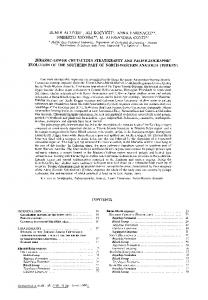
During the earliest Phanerozoic, Australia is located at equatorial latitudes. Fossil data are sparse globally in the Cambrian and Ordovician (Fig. 4a, b and c) as well as data constraining the corresponding maps of the Palaeogeographic Atlas of Australia (Totterdell, 2002). The eastern shelf of Australia transforms from an abyssal environment (Fig. 4a) to bathyal-abyssal sea (Fig. 4b and c) with an east–west band of shallow marine and coastal depositional environments through the central portion of the continent forming the westernmost limit of the Tasman Line (Fig. 5). Fossil assemblages indicate marine environments such as carbonate and reef, buildup or bioherm environments, which correlate with the shallow marine environment from the paleogeographic model. Numerous erosional and non-depositional areas are present within the Australian continent from the late Silurian (Fig. 4d). Paleoenvironments inferred from fossil assemblages indicate and correlate with bands of marine environments along southeastern Australia (Fig. 4d). During the early Silurian, the deep-water environments previously observed along eastern Australia retreated and deformation and regional uplift occurred, associated with the Benambran Orogeny (Collins and Hobbs, 2001; Totterdell, 2002), followed by crustal extension in areas of eastern Australia, which occurred through the Silurian. Similarly, biofacies data correlate well with Australian paleogeography during the Early to Middle Devonian (Fig. 4e); the eastern margin is classified as marine bathyal-abyssal and marine shallow (Fig. 4e), and fossil assemblages similarly indicate a marine depositional environment at this time, including carbonate and basinal (siliciclastic) settings. Fossil data are available for most of the eastern inundated areas of the Australian margin but sparse for the remainder of the continent, largely due to the erosional conditions on land.
www.biogeosciences.net/10/1529/2013/
During the latest Devonian to early Carboniferous, the Palaeogeographic Atlas of Australia indicates the retreat of shallow marine environments along eastern Australia (Totterdell, 2002), and spatially corresponding fossil paleoenvironmental data support a marine environment, based on shallow subtidal, carbonate and marine indicators (Fig. 4f). The remaining paleogeography of Australia is unclassified, with an erosional region in central Australia. Global fossil data coverage for this time slice is poor and may be related to the Late Devonian major extinction event (Golonka et al., 2006). A global oceanic anoxic event (OAE) and icehouse conditions, initiated in the Devonian, prevailed into the Carboniferous (Golonka et al., 2006). The erosional conditions associated with the paleogeographic model continue into the late Carboniferous and early Permian. Fossil data coverage is poor during the Carboniferous, with only one fossil data point located within the Australian continent and indicating a lacustrine setting, which may be the local base level (sedimentary depocentre) (Fig. 4g). However, insufficient paleobiology data are available to define the extent of the lacustrine environment. Icehouse conditions continued into the late Carboniferous, where the southern polar ice cap reached its maximum, covering regions of Australia, Antarctica, southern India and Arabia, Madagascar, Africa, and southeastern South America (Golonka et al., 2006). Fossil data coverage during the early Permian correlates with the shallow marine environments present along eastern Australia and pockets of western Australia during the early Permian (Fig. 4h). Paleogeography is predominantly unclassified during the Triassic and Jurassic (Fig. 4i, j and k), and fossil assemblages located within Australia are sparse, possibly attributed to the late Permian extinction event (Benton and Twitchett, 2003), environmental conditions and/or biased sampling. Increased fossil data or further proxies are required to infer the extent paleoenvironments from fossil. Available biofacies during the Cretaceous are more expansive and suggest terrestrial and shallow
Biogeosciences, 10, 1529–1541, 2013
1534
N. Wright et al.: Towards community-driven paleogeographic reconstructions
A. Early Cambrian (520 Ma)
C. late Middle - Late Ordovician (452 Ma)
B. Latest Cambrian - Early Ordovician (488 Ma)
30°N
30°N
20°E
30°N
180°
0°
0°
0°
1,000 2,000
0
30°N
30°N
30°N
20°E
0°
0°
0
30°N
30°N
30°N
0°
0°
0°
0°
160°W
30°S
0°
30°S
0°
4,000 Kilometers
0
1,000 2,000
0
N. Thanetian - Ypresian (53 Ma)
M. Late Cretaceous (90 Ma)
30°N
0°
0°
0°
0°
0°
160°W
30°S
1,000 2,000
0
1,000 2,000
180°
0°
0°
30°S
1,000 2,000
30°N
0°
160°W
30°S
0
4,000 Kilometers
20°E
0°
4,000 Kilometers
1,000 2,000
30°N
180°
0°
30°S
4,000 Kilometers
30°N
0°
160°W
30°S
30°S
0
0°
0
P. Tortonian - Gelasian (6 Ma)
20°E
180°
160°W 30°S
4,000 Kilometers
30°N
30°N
20°E
180°
0°
30°S
O. Priabonian - Rupelian (33 Ma)
30°N
30°N
20°E
1,000 2,000
180°
0°
30°S
4,000 Kilometers
30°N
0°
160°W
30°S
4,000 Kilometers
30°N
0°
30°S
1,000 2,000
20°E
180°
0°
160°W
30°S
0
L. Early Cretaceous (126 Ma)
30°N
20°E
0°
160°W 30°S
4,000 Kilometers
30°N
180°
0°
30°S
K. Middle Jurassic - Late Jurassic (152 Ma)
30°N
20°E
180°
180°
0°
30°S
1,000 2,000
30°N
0°
160°W
30°S
0
4,000 Kilometers
20°E
0°
4,000 Kilometers
1,000 2,000
30°N
180°
0°
J. Early Jurassic - earliest Middle Jurassic (195 Ma)
20°E
1,000 2,000
1,000 2,000
30°N
0°
30°S
4,000 Kilometers
I. Early - earliest Late Triassic (232 Ma)
0
H. Early Permian (277 Ma)
30°N
160°W
30°S
30°S
30°S
4,000 Kilometers
20°E
0°
0°
160°W
30°S
1,000 2,000
160°W
30°S
G. Late Carboniferous (302 Ma)
180°
0°
0°
0
0
0°
0°
30°S
4,000 Kilometers
30°N
20°E
180°
1,000 2,000
1,000 2,000
180°
0°
160°W
30°S
F. latest Devonian - Early Carboniferous (348 Ma)
E. Early - Middle Devonian (396 Ma)
0
0°
30°N
20°E
0°
30°S
4,000 Kilometers
30°N
180°
0°
160°W
30°S
30°N
20°E
0°
0°
30°S
0
180°
0°
160°W
30°S
30°N
30°N
20°E
D. Late Silurian (425 Ma)
160°W
30°S
4,000 Kilometers
30°S
0
1,000 2,000
4,000 Kilometers
Legend Biofacies
Paleogeography Crater lake
Dune
Interdune
Loess
Platform/shelf-margin reef
Submarine fan
Basin reef
Crevasse splay
Eolian indet.
Intrashelf/intraplatform reef
Marginal marine indet.
Pond
Tar
Basinal (carbonate)
Deep subtidal indet.
Estuary/bay
Karst indet.
Marine indet.
Prodelta
Terrestrial indet.
Basinal (siliceous)
Deep subtidal ramp
Fine channel fill
Lacustrine - large
Mire/swamp
Reef, buildup or bioherm
Transition zone/lower shoreface
Basinal (siliciclastic)
Deep subtidal shelf
Fissure fill
Lacustrine - small
Offshore
Sand shoal
Wet floodplain
Land depositional fluvial-lacustrine
Carbonate indet.
Deep-water indet.
Floodplain
Lacustrine delta front
Offshore indet.
Shale
Data Coverage
Land depositional glacial
Cave
Delta front
Fluvial indet.
Lacustrine delta plain
Offshore ramp
Shallow subtidal indet.
Fluvial-deltaic indet.
Lacustrine deltaic indet.
Offshore shelf
Shoreface
Land depositional unclassified
Fluvial-lacustrine indet.
Lacustrine indet.
Open shallow subtidal
Sinkhole
Land environment erosional
Foreshore
Lagoonal
Paralic indet.
Slope
Land environment unclassified
Alluvial fan
Channel
Delta plain
Channel lag Coarse
Deltaic indet.
Coarse channel fill
Dolomitic
Glacial
Lagoonal/restricted shallow subtidal
Perireef or subreef
Slope/ramp reef
Coastal indet.
Dry floodplain
Interdistributary bay
Levee
Peritidal
Spring
Coastal depositional deltaic Coastal depositional intertidal-supratid Coastal depositional paralic Land depositional aeolian Land depositional fluvial
Land depositional lacustrine Land depositional playa
Marine abyssal Marine bathyal-abyssal Marine shallow Marine very shallow
Fig. 4. Phanerozoic global plate reconstructions with Australian paleogeography and fossil indicators documenting the equatorial position of Australia in the Cambrian, followed by a south polar position by the end of the Paleozoic. The breakup of Pangea resulted in the northward motion of Australia back towards the equator. Increments are based on time slices presented by Golonka et al. (2006). Ages in the figure refer to the reconstruction time of each map.
Biogeosciences, 10, 1529–1541, 2013
www.biogeosciences.net/10/1529/2013/
N. Wright et al.: Towards community-driven paleogeographic reconstructions
1535
a)
b)
30°S
30°S
35°S
35°S
125°E
130°E
135°E
125°E
c)
130°E
135°E
d) ?
?
? ?
30°S
30°S
?
Interpreted
? ?
?
?
Snowy Mountains Block 35°S
35°S
125°E
130°E
135°E
125°E
130°E
135°E
Legend Lithology
Biofacies Carbonate indet.
Frog Hollow Formation
Marine indet.
Jesse Limestone
Reef, buildup or bioherm
Humevale Siltstone
Slope
Formation
McIvor Sandstone Mount Ida Formation
Bell Point Limestone
Taemas Limestone
Brogans Creek Limestone
Taravale Mudstone
Buchan Caves Limestone
Unspecified
Coopers Creek Limestone
Waratah Limestone
marine environments within Australia (Fig. 4l and m), and predominately correlate with the withdrawing sea in northeast Australia indicated by the Palaeogeographic Atlas of Australia (Totterdell, 2002). During the Cenozoic, the paleogeography of Australia is predominantly an erosional land environment with variations in fluvial environment distribution (Fig. 4n, o and p). Biofacies within Australia are sparse, however their distribution corresponds with paleogeographic descriptors.
www.biogeosciences.net/10/1529/2013/
Framestone Grainstone
Land depositional fluvial Land environment erosional Land environment unclassified Marine abyssal
Lime mudstone
Marine bathyal-abyssal
Limestone
Marine shallow
Not reported
Devonian Outcrops (present-day)
Sandstone
Political Boundaries (for reference)
Shale Siltstone
Fair Hill Formation
Fig. 5. (a) Data coverage with 100 km buffer (green) from the Paleobiology Database for Australia, with basin outlines and political boundaries as reference. Temporal coverages of fossil collections are for (b) general, (c) carbonate, (d) siliciclastic marine, and (e) terrestrial fossil collections, showing that the dataset sufficiently represents Phanerozoic biofacies.
Conglomerate
Paleogeography
Fig. 6. (a) Paleogeographic reconstruction at 402 Ma (Early Devonian/Emsian) from Geoscience Australia Palaeogeographic Atlas of Australia with inferred paleoenvironments from fossils, present-day Devonian outcrops and reconstructed political boundaries for reference. Fossil specimens (including echinoderms, shell and skeletal fragments) in New South Wales and Victoria indicate shallow marine environments. The fossils have well-constrained temporal descriptors indicative of Early Devonian times, with a number of specimens better tied to Emsian times based on conodont zones (i.e. Eognathodus trilinearis, Polygnathus dehicens, etc.). (b) Paleogeographic reconstruction with formation types indicated, based on fossil metadata. (c) Paleogeographic reconstruction with fossil lithologies indicated, based on metadata. (d) A reinterpretation of Emsian paleogeography, suggesting marine environments persisted until at least Emsian times in Victoria, and linking the marine inundation to the Yass Shelf to be more consistent with the interpretations of Webby (1972) and the overall N–S striking convergent margin of Australia at this time.
3.2
Emsian case study
An Emsian (402 Ma) paleogeographic reconstruction (Fig. 6a) highlights the potential benefits of using biological Biogeosciences, 10, 1529–1541, 2013
1536
N. Wright et al.: Towards community-driven paleogeographic reconstructions
Paleogeography
Marine shallow
Marine abyssal
Land environment unclassified
Land environment erosional Carbonate indeterminate
Marginal marine indeterminate
Marine indeterminate
Perireef or subreef
Reef, buildup or bioherm
Shoreface
Slope
Biofacies
Fig. 7. Biofacies and paleogeographic associations at 402 Ma (Early Devonian, Emsian times) highlight the discordance between the marine setting indicated by the fossil collections and the Australian paleogeography at this time (red circles). Agreement between the paleogeographic model and fossil assemblages is also indicated (green circles). The fossil collections, as the seed points, were used to extract the paleogeography to create a time series for the purposes of data mining.
indicators of paleoenvironment, as there are significant mismatches between the proposed “Land environment unclassified” in the paleogeography model and the marine fossils (Fig. 7), particularly in the state of Victoria. The fossils have good temporal constraints at stage level, indicative of Early Devonian age, with a number of them more specifically Emsian in age based on conodont horizons – namely Eognathodus trilinearis and Polygnathus dehicens. The Emsian fossils are found in the Bell Point, Buchan Caves and the Waratah Limestones (Fig. 6b) with shell and skeletal fragments. The Early Devonian fauna in central Victoria are found in the Humevale formation containing echinoderm fragments. Lithological investigations support marine interpretation, indicating the fossils were found in limestones, siltstones and sandstone (Fig. 6c). However, challenges arise when comparing the temporal range of fossils and associated formations. Fossil metadata contains a larger temporal range compared to the associated formation temporal range found in published research, and this may restrict possible paleogeographic interpretations. A generalised stratigraphic column (Fig. 8) focused on formations that were deposited during the reconstruction time (Fig. 6b). For example, Coopers Creek Formation and Humevale Siltstone ceased deposition in the Pragian (Rehfisch and Webb, 1993; Webby, 1972) (Fig. 8) and were not used for the Emsian interpretations. The stratigraphic and fossil data can be used to expand the paleogeographic model at this time, with a possible expansion of inundation into southern New South Wales (NSW) and Victoria Biogeosciences, 10, 1529–1541, 2013
(Fig. 6d). This interpretation included formations that were present during the mid-Emsian, such as Taravale Formation and Taemas Limestone, whilst formations including Coopers Creek Formation and Humevale Siltstone were excluded due to the disagreement in age. 4
Discussion
Linking the paleogeographic history of Australia with biofacies from the Paleobiology Database demonstrates how a paleogeographic model can be tested and potentially improved using empirical, qualitative and quantitative approaches, although it should be noted that paleogeographic maps cannot be created solely from fossils obtained from the Paleobiology Database. However, the global Paleobiology Database forms an additional data layer to help constrain existing paleogeographic interpretations that were agnostic to the global fossil dataset. Highlighting associations between the fossil data and paleogeography has allowed us to highlight inconsistencies between raw data (fossil collections) and the paleogeographic interpretations. Although the data coverage for the paleobiology data is imperfect for Australia in comparison to Eurasia and North America, it is an exemplary first-order tool to constrain the evolution of continental inundation histories in the Phanerozoic.
www.biogeosciences.net/10/1529/2013/
N. Wright et al.: Towards community-driven paleogeographic reconstructions KINGLAKE WEST
AGE
TYERS
WARATAH BAY
BUCHAN
MURUMBIDGEE WEE JASPER
EIFELIAN Taravale Fm Murrindal Lmst.
EMSIAN Walhalla Group
PRAGIAN
Buchan Caves Limestone
Waratah Lmst.
Killingworth Fm Flowerdale member
Humevale Siltstone
Bells Pt Lmst.
Coopers Creek Formation
Taemas Limestone
Taemas Limestone
Majurgong Fm
Majurgong Fm
Cavan Bluff Lmst.
Cavan Bluff Lmst.
Snowy River Volcanics
Fig. 8. Generalised correlation column of stratigraphy in Victoria and southern New South Wales. Description of regions were based on formations described in Webby (1972) and Philip and Pedder (1967). Adjustments were made to the temporal range of the Buchan Caves Limestone (Holloway, 1996) and Coopers Creek Formation (Rehfisch and Webb, 1993).
4.1
Refining paleogeographic models of Australia using paleobiology
The paleogeographic evolution of Australia is punctuated by a number of significant periods that include the Paleozoic growth of the eastern Australian continent and the inundation of Australia in the mid-Cretaceous from the late Aptian to the Campanian (Gurnis et al., 1998). 4.1.1
Early Devonian (⇠ 419–393 Ma)
Biofacies that have a well-defined temporal range and paleoenvironmental association can be used to refine existing models of paleogeography. As an example of such an approach, we propose that the inundation of Victoria and a portion of NSW in the Early Devonian lasted until at least the Emsian. We infer that the marine deposition at the Yass Shelf formed a north–south marine corridor that partially separated the Snowy Mountains Block from the mainland (Fig. 6d). The Devonian outcrops at present day suggest sedimentation continued into the Emsian, and is largely consistent with the interpretations of Webby (1972) and Veevers (2004) as well as the north–south geometry of the convergent margin along eastern NSW in the Paleozoic (Aitchison and Buckman, 2012). Our results indicate that the shallow marine setting persisted until the onset of the Tabberabberan Orogeny (390–380 Ma) in the Middle Devonian (Collins, 2002; Gray and Foster, 1997). 4.1.2
Cretaceous (145–65 Ma)
The Cretaceous was a significant period of marine inundation in Australia; maximum flooding occurred during the late Aptian to early Albian (120 to 110 Ma) and had predominantly eased by the Campanian (80 to 70 Ma) (Gurnis et al., 1998). Such flooding occurred across large expanses of the continental region east of the cratonic portion of Australia www.biogeosciences.net/10/1529/2013/
1537
marked by the Tasman Line. The northeastward motion of Australia over a descending Pacific-derived slab induced a strong negative dynamic topography signal that accentuated flooding from the mid-Cretaceous sea level highstand (DiCaprio et al., 2009; Gurnis et al., 1998; Heine et al., 2010; Matthews et al., 2011). Well-constrained models of paleogeography are an important validating mechanism for numerical models of dynamic topography, as demonstrated by Gurnis et al. (1998) in the study of the Cretaceous inundation of Australia (Fig. 9). Subsidence from dynamic topography is distinguishable from loading-induced subsidence as it can be reversed if the negative dynamic topography signal diminishes (Gurnis et al., 1998). In the case of eastern Australia, a Pacific-derived slab sinking beneath eastern Australia imparts up to 350 m of predicted subsidence from geodynamic models on the region underlying the Eromanga Basin between 120 and 110 Ma (Gurnis et al., 1998), but this effect diminishes by 60 Ma as the depth of the sinking slab increases due to the lower viscous coupling between the slab and the lithosphere. As a result, the inundation of eastern Australia retreated due to ⇠ 200 m of uplift caused by the waning negative dynamic topography signal in an overall eustatic sea level highstand (Seton et al., 2009). The paleogeographic model indicates inundation in the northeast of the Australian continent from 139 Ma; this flooding progressively covers a large portion of eastern Australia, peaking at ⇠ 123 Ma. The shallow marine environments (water depths of up to 200 m) begin retreating after 100 Ma and disappear by 80 Ma (Fig. 9), to be replaced by fluvial and other terrestrial depositional environments. Paleobiology data largely correlate with the paleogeographic model. Minimal inundation is present at 80 Ma, and sparse paleobiology data is available for this time, suggesting that the negative dynamic topography signal diminished by ⇠ 100 Ma or that eustatic sea level fell to induce a marine regression. Additionally, the inundation history is recorded in the fossil collections from the Eromanga Basin, with a distinct peak of fossil preservation coinciding with the Cretaceous inundation (Fig. 10). 4.2
Testing plate motions using paleogeography and biofacies
Paleogeography and biofacies embedded within plate reconstructions can be used to uncover inconsistencies and help refine the plate motion model. The Cretaceous period records significant changes in the tectonic forces acting on the Australian plate, largely driven by the breakup of Gondwana and the subduction of Pacific material along Australia’s eastern margin (Veevers, 2012). The relative plate motions suggest rifting between Australia and greater India began at ⇠ 165 Ma, consistent with interpretations of seismic sections that indicate rift-related normal faulting penetrated Late Jurassic sedimentary sequences (Song and Cawood, 2000) and syn-rift sediments in the southern Perth Basin (Veevers, 2012). However, the rift-related inundation of this margin Biogeosciences, 10, 1529–1541, 2013
1538
N. Wright et al.: Towards community-driven paleogeographic reconstructions
Fig. 9. Paleogeographic reconstructions suggest that Cretaceous inundation of central eastern Australia peaked by ⇠ 120 Ma, and the fossil indicators hint at pockets of shallow marine environments persisting beyond 100 Ma. The eastward sweeping negative dynamic topography system from a sinking Pacific-derived slab has been linked to the inundation pattern, better modelled by Model C (blue) than Model B (purple) in the geodynamic modelling results of Gurnis et al. (1998), highlighting how paleogeography can be used to validate numerical model predictions of basin evolution.
occurs much later at ⇠ 139 Ma based on the paleogeographic model. The discrepancy between the Late Jurassic onset of rifting and delayed submergence may be accounted for by the oblique style of rifting, which resulted in abundant strikeslip faulting (Song and Cawood, 2000), and therefore relatively little lithospheric extension for much of the rift phase, thus delaying subsidence and inundation until a few million years before breakup. Additionally, seafloor spreading initiated some time between ⇠ 136 and 130 Ma (Gibbons et al., 2012; Robb et al., 2005), thus accentuating the inundation of the margin that is observed in the paleogeographic reconstruction. Although the plate motion model is consistent with the rifting history between Australia–India–Antarctica, Golonka’s (2007) plate motion model may need refinement for the Cretaceous Australia–Antarctica rifting history. The paleogeographic model suggests that inundation of the western Australia–Antarctic margin initiates by 125 Ma and propagates eastward, reaching Tasmania by 100 Ma, consistent with a previous onset of rifting in the Valanginian (Totterdell and Bradshaw, 2004). The progressive submergence of the margin reflects the eastward propagation of the rift, as Biogeosciences, 10, 1529–1541, 2013
Fig. 10. Temporal coverage of eastern Australian basins (EA) and the Eromanga Basin (EB). Much of the sampled collections are on the outskirts of the Eromanga Basin with data gaps that may be related to sampling gaps, orogenic episodes and the influence of glaciations on eastern Australia during the late Paleozoic.
originally suggested by Mutter et al. (1985), that may be accentuated by the global mid-Cretaceous seafloor spreading pulse resulting in a eustatic sea level highstand (Seton et al., 2009). However, the peak of the sea level highstand and seafloor spreading pulse post-dates the peak inundation of the rifted Australia–Antarctica margin, and suggests that the progressive inundation was mainly rift-related. The prebreakup fit in the Golonka (2007) model requires refinement to minimise continental overlaps and initiation of rifting at ⇠ 121 Ma, as demonstrated by Williams et al. (2011) for the Australian–Antarctic conjugate margins. 4.3
Data coverage and resolution
Data coverage of the eastern coast of Australia follows the band of Cretaceous inundation, resulting in reasonable spatio-temporal coverage of the region (Figs. 5 and 10). At least five sizeable gaps in the temporal coverage are present in the paleobiology, and we suggest that some of the temporal gaps are a result of the episodic orogenic events related to the Tasman Orogenic System in the Paleozoic, leading to the eastward growth of the Australian continent in an accretionary convergent margin setting (Coney et al., 1990; Crawford et al., 2003; Henderson et al., 2011; Solomon and Griffiths, 1972). The lack of fossil assemblages elsewhere in Australia is a result of biased sampling and the environment type at the time, and the denudation patterns that resulted in exposing cratonic portions of the continent to potentially remove Phanerozoic fossil-bearing sediments. The combination of paleobiology, plate reconstructions and the www.biogeosciences.net/10/1529/2013/
N. Wright et al.: Towards community-driven paleogeographic reconstructions paleogeography in GPlates has allowed us to use a novel approach to test the correlation of existing paleogeographic maps and fossil indicators of environments. The use of GPlates is significant, as paleogeographic maps can be dynamic and updated with relative ease based on new data, rather than the reliance on static maps that are revised infrequently. GPlates also allows the incorporation of multiple layers of proxy data to increase the confidence of paleogeographic reconstructions to test numerical model predictions of continental inundation patterns through time. Spatio-temporal data coverage is a considerable concern in the interpretation of the fossil record since poor sampling is difficult to distinguish from lack of fossil preservation. Regions in the Northern Hemisphere, such as North America and Europe, typically display a greater abundance of fossil data compared to areas in the present day Southern Hemisphere, such as Australia. Such discrepancies may be the result of biased sampling and/or preservation and environmental conditions. Spatio-temporal data coverage in Australia has predominantly been restricted to eastern Australia, and suggests at least five temporal gaps in coverage (Fig. 10). Paleogeographic reconstructions were further restricted by the lack of variation in fossil assemblage environments: paleobiology data are predominantly available for marine paleoenvironments. As a result, other proxy data are required for constraining paleoenvironments with low biological preservation potential – such as orogenic settings that can be constrained using metamorphic assemblages and denudation histories in proximal basins. Paleogeographic maps can be further refined by incorporating additional published paleoenvironment indicators, including well logs and other timedependent datasets using GPlates. Future directions include a greater analysis of paleogeography on a global scale as indicated by fossil paleoenvironments, including the effect of glaciations, continental inundations and mass extinction throughout the Phanerozoic on fossil assemblages. In particular, such an approach would be best suited for European and North American paleogeographic reconstructions due to the higher spatio-temporal coverage in the fossil record (Hannisdal and Peters, 2011). Glaciations have played a major role in global climate throughout the Phanerozoic, and may have influenced the preservation of organisms. The glaciation throughout the latest Devonian to early Permian (Scotese et al., 1999) may be responsible for the few and scattered fossil assemblages found globally in the late Paleozoic. Similarly, the inundation of continental regions can influence preservation of organisms, based on the availability of desirable preservation conditions, and should be noted in global and regional observations in plate reconstructions. Sudden increases in fossil abundance temporally and spatially may reflect local environmental changes and preservation conditions, rather than an increase in biodiversity or biologic density. Specifically, the inundation history of Australia, throughout the Cretaceous, is associated with increased spatial and temporal fossil www.biogeosciences.net/10/1529/2013/
1539
preservation in the eastern Australian basins (Fig. 10). The increased inundation of the continent and a biased biological preservation during this time interval is consistent with a mid-Cretaceous seafloor spreading pulse and increase in eustatic sea level (Seton et al., 2009). 5
Conclusions
Our approach demonstrates that paleogeographic and plate reconstructions can be improved and refined using paleoenvironments indicated by fossils from the global Paleobiology Database. Our novel application of spatio-temporal data mining can be used to identify inconsistencies between paleogeography and fossil data. Our approach allows the incorporation of multiple proxy datasets to help refine plate and paleogeographic reconstructions, and enables the creation of a new generation of digital and interactive models that allow users to create dynamic maps that are expandable and testable, and that take advantage of regularly maintained databases. Sediments and related fossil assemblages are largely confined to basins, and this only provides indirect constraints for elevated topographic regions representing sediment sources. As a result, in the future it will be desirable to incorporate proxies of elevation, such as paleoaltimetry estimates based on paleobiological indicators (i.e. leaf morphologies and stomata densities) (McElwain, 2004), and stable and metamorphic assemblage isotopes (Blisniuk and Stern, 2005). GPlates is evolving into an open innovation platform with a plugin infrastructure and an extended information model (M¨uller et al., 2012) that will enable the creation of adaptable and interactive paleogeographic maps that are expandable in order to assimilate growing chronostratigraphic data systems (Sikora et al., 2006) in addition to paleobiology data. Supplementary material related to this article is available online at: http://www.biogeosciences.net/10/ 1529/2013/bg-10-1529-2013-supplement.zip.
Acknowledgements. The project was supported by ARC grants FL0992245 and DP0987713. Thomas Landgrebe provided help with the data mining methodology. This is Paleobiology Database publication #163. Edited by: W. Kiessling
Biogeosciences, 10, 1529–1541, 2013
1540
N. Wright et al.: Towards community-driven paleogeographic reconstructions
References Aitchison, J. C. and Buckman, S.: Accordion vs. quantum tectonics: Insights into continental growth processes from the Paleozoic of eastern Gondwana, Gondwana Res., 22, 674–680, 2012. Benton, M. J. and Twitchett, R. J.: How to kill (almost) all life: the end-Permian extinction event, Trends Ecol. Evol., 18, 358–365, 2003. Blisniuk, P. M. and Stern, L. A.: Stable isotope paleoaltimetry: A critical review, Am. J. Sci., 305, 1033–1074, 2005. Cocks, L. R. M. and Torsvik, T. H.: Earth geography from 500 to 400 million years ago: a faunal and palaeomagnetic review, J. Geol. Soc., 159, 631–644, 2002. Collins, W. J.: Nature of extensional accretionary orogens, Tectonics, 21, 1024, doi:10.1029/2000TC001272, 2002. Collins, W. J. and Hobbs, B. E.: What caused the Early Silurian change from mafic to silicic (S-type) magmatism in the eastern Lachlan Fold Belt?, Austr. J. Earth Sci., 48, 25–41, doi:10.1046/j.1440-0952.2001.00837.x, 2001. Coney, P. J., Edwards, A., Hine, R., Morrison, F., and Windrim, D.: The regional tectonics of the Tasman orogenic system, eastern Australia, J. Struct. Geol., 12, 519–543, 1990. Crawford, A., Meffre, S., and Symonds, P.: 120 to 0 Ma tectonic evolution of the southwest Pacific and analogous geological evolution of the 600 to 220 Ma Tasman Fold Belt System, Special Papers – Geological Society of America, 383–404, 2003. DiCaprio, L., Gurnis, M., and M¨uller, R. D.: Long-wavelength tilting of the Australian continent since the Late Cretaceous, Earth Planet. Sc. Lett., 278, 175–185, 2009. Direen, N. G. and Crawford, A. J.: The Tasman Line: where is it, what is it, and is it Australia’s Rodinian breakup boundary?, Austr. J. Earth Sci., 50, 491–502, doi:10.1046/j.14400952.2003.01005.x, 2003. Donnadieu, Y., Godd´eris, Y., Pierrehumbert, R., Dromart, G., Fluteau, F., and Jacob, R.: A GEOCLIM simulation of climatic and biogeochemical consequences of Pangea breakup, Geochem. Geophy. Geosys., 7, Q11019, doi:10.1029/2006GC001278, 2006. Ford, D. and Golonka, J.: Phanerozoic paleogeography, paleoenvironment and lithofacies maps of the circum-Atlantic margins, Mar. Petrol. Geol., 20, 249–285, 2003. Gibbons, A. D., Barckhausen, U., van den Bogaard, P., Hoernle, K., Werner, R., Whittaker, J. M., and M¨uller, R. D.: Constraining the Jurassic extent of Greater India: Tectonic evolution of the West Australian margin, Geochem. Geophy. Geosys., 13, Q05W13, doi:10.1029/2011GC003919, 2012. Golonka, J.: Late Triassic and Early Jurassic palaeogeography of the world, Palaeogeogr. Palaeocl., 244, 297–307, 2007. Golonka, J., Krobicki, M., Pajak, J., Van Giang, N., and Zuchiewicz, W.: Global Plate Tectonics and Paleogeography of Southeast Asia, edited by: Doktor, M., Faculty of Geology, Geophysics and Environmental Protection, AGH University of Science and Technology, Arkadia, Krakow, 128 pp., 2006. Gradstein, F. M. and Ogg, J.: Geologic Time Scale 2004 – why, how, and where next!, Lethaia, 37, 175–181, 2004. Gradstein, F. M., Ogg, J. G., Smith, A. G., Bleeker, W., and Lourens, L. J.: A new geologic time scale, with special reference to Precambrian and Neogene, Episodes, 27, 83–100, 2004. Gray, D. R. and Foster, D. A.: Orogenic concepts-application and definition: Lachlan Fold Belt, eastern Australia, Am. J. Sci., 297,
Biogeosciences, 10, 1529–1541, 2013
859–891, 1997. Gurnis, M., Muller, R. D., and Moresi, L.: Cretaceous vertical motion of Australia and the Australian-Antarctic discordance, Science, 279, 1499–1504, 1998. Gyllenhaal, E. D., Engberts, C. J., Markwick, P. J., Smith, L. H., and Patzkowsky, M. E.: The Fujita-Ziegler model: a new semiquantitative technique for estimating paleoclimate from paleogeographic maps, Palaeogeogr. Palaeocl., 86, 41–66, 1991. Hallam, A. and Cohen, J.: The case for sea-level change as a dominant causal factor in mass extinction of marine invertebrates [and discussion], Philos. T. Roy. Soc. B, 325, 437–455, 1989. Hallam, A. and Wignall, P.: Mass extinctions and sea-level changes, Earth-Sci. Rev., 48, 217–250, 1999. Hannisdal, B. and Peters, S. E.: Phanerozoic Earth System Evolution and Marine Biodiversity, Science, 334, 1121–1124, 2011. Heine, C., M¨uller, R. D., Steinberger, B., and DiCaprio, L.: Integrating deep Earth dynamics in paleogeographic reconstructions of Australia, Tectonophysics, 483, 135–150, doi:10.1016/j.tecto.2009.08.028, 2010. Henderson, R. A., Innes, B. M., Fergusson, C. L., Crawford, A. J., and Withnall, I. W.: Collisional accretion of a Late Ordovician oceanic island arc, northern Tasman Orogenic Zone, Australia, Austr. J. Earth Sci., 58, 1–19, doi:10.1080/08120099.2010.535564, 2011. Holloway, D. J.: New Early Devonian Styginid Trilobites from Victoria, Australia, with Revision of Some Spinose Styginids, J. Paleontol., 70, 428–438, 1996. Matthews, K. J., Hale, A. J., Gurnis, M., M¨uller, R. D., and DiCaprio, L.: Dynamic subsidence of Eastern Australia during the Cretaceous, Gondwana Res., 19, 372–383, 2011. McElwain, J. C.: Climate-independent paleoaltimetry using stomatal density in fossil leaves as a proxy for CO2 partial pressure, Geology, 32, 1017–1020, 2004. Metcalfe, I.: Gondwanaland origin, dispersion, and accretion of East and Southeast Asian continental terranes, J. S. Am. Earth Sci., 7, 333–347, 1994. Miller, K. G., Kominz, M. A., Browning, J. V., Wright, J. D., Mountain, G. S., Katz, M. E., Sugarman, P. J., Cramer, B. S., ChristieBlick, N., and Pekar, S. F.: The phanerozoic record of global sealevel change, Science, 310, 1293–1298, 2005. M¨uller, R. D., Sdrolias, M., Gaina, C., Steinberger, B., and Heine, C.: Long-term sea-level fluctuations driven by ocean basin dynamics, Science, 319, 1357–1362, 2008. M¨uller, R. D., Cannon, J., Landgrebe, T. C. W., and Qin, X.: An open innovation platform for deep time spatio-temporal knowledge-discovery, 6th eResearch Australasia Conference, Sydney, 28 October–1 Novemver 2012, 2012. Mutter, J. C., Hegarty, K., Cande, S. C., and Weissel, J. K.: Breakup between Australia and Antarctica: a brief review in the light of new data, Tectonophysics, 114, 255–279, 1985. Philip, G. M. and Pedder, A. E.: A Correlation of Some Devonian Limestones of New South Wales and Victoria, Geol. Mag., 104, 232–239, doi:10.1017/S0016756800048743, 1967. Qin, X., M¨uller, R. D., Cannon, J., Landgrebe, T. C. W., Heine, C., Watson, R. J., and Turner, M.: The GPlates Geological Information Model and Markup Language, Geosci. Instrum. Method. Data Syst., 1, 111–134, doi:10.5194/gi-1-111-2012, 2012. Rehfisch, M. W. and Webb, J. A.: The Early Devonian Coopers Creek Limestone: A deep-water redeposited limestone in the
www.biogeosciences.net/10/1529/2013/
N. Wright et al.: Towards community-driven paleogeographic reconstructions Melbourne Trough, southeastern Australia, Austr. J. Earth Sci., 40, 575–589, doi:10.1080/08120099308728105, 1993. Robb, M. S., Taylor, B., and Goodliffe, A. M.: Re-examination of the magnetic lineations of the Gascoyne and Cuvier Abyssal Plains, off NW Australia, Geophys. J. Int., 163, 42–55, 2005. Ross, M., Scotese, C., and Otto-Bliesner, B.: Phanerozoic paleoclimate simulations: A comparison of the parametric climate model and the low resolution climate model, Geol. Soc. Am., Abstracts with Programs;United States, 24, p. 89, 1992. Scotese, C. R.: A Continental Drift Flipbook, J. Geol., 112, 729– 741, doi:10.1086/424867, 2004. Scotese, C. R., Boucot, A. J., and McKerrow, W. S.: Gondwanan palaeogeography and palaeoclimatology, J. Afr. Earth Sci., 28, 99–114, 1999. Seton, M., Gaina, C., M¨uller, R., and Heine, C.: Mid-Cretaceous seafloor spreading pulse: Fact or fiction?, Geology, 37, 687–690, 2009. Seton, M., M¨uller, R., Zahirovic, S., Gaina, C., Torsvik, T., Shephard, G., Talsma, A., Gurnis, M., Turner, M., and Chandler, M.: Global continental and ocean basin reconstructions since 200 Ma, Earth-Sci. Rev., 113, 212–270, 2012. Sikora, P. J., Ogg, J. G., Gary, A., Cervato, C., Gradstein, F., Huber, B. T., Marshall, C., Stein, J. A., and Wardlaw, B.: An integrated chronostratigraphic data system for the twenty-first century, Geoinformatics: data to knowledge, 397, 53–59, 2006. Solomon, M. and Griffiths, J.: Tectonic evolution of the Tasman Orogenic zone, eastern Australia, Nature, 237, 3–6, 1972. Song, T. and Cawood, P. A.: Structural styles in the Perth Basin associated with the Mesozoic break-up of Greater India and Australia, Tectonophysics, 317, 55–72, 2000.
www.biogeosciences.net/10/1529/2013/
1541
Stanley, S. M.: Paleozoic mass extinctions; shared patterns suggest global cooling as a common cause, Am. J. Sci., 288, 334–352, doi:10.2475/ajs.288.4.334, 1988. Torsvik, T. H. and Van der Voo, R.: Refining Gondwana and Pangea Palaeogeography: Estimates of Phanerozoic non-dipole (octupole) fields, Geophys. J. Int., 151, 771–794, 2002. Totterdell, J. M.: Palaeogeographic Atlas of Australia, Geoscience Australia, 2002. Totterdell, J. M. and Bradshaw, B.: The structural framework and tectonic evolution of the Bight Basin, Eastern Australasian Basins Symposium II, Adelaide, 41–61, 2004. Van der Voo, R.: The reliability of paleomagnetic data, Tectonophysics, 184, 1–9, 1990. Veevers, J. J.: Gondwanaland from 650–500 Ma assembly through 320 Ma merger in Pangea to 185–100 Ma breakup: supercontinental tectonics via stratigraphy and radiometric dating, EarthSci. Rev., 68, 1–132, doi:10.1016/j.earscirev.2004.05.002, 2004. Veevers, J. J.: Reconstructions before rifting and drifting reveal the geological connections between Antarctica and its conjugates in Gondwanaland, Earth-Sci. Rev., 111, 249–318, 2012. Webby, B. D.: Devonian geological history of the Lachlan Geosyncline, J. Geol. Soc. Austr., 19, 99–123, 1972. Wegener, A.: Die Entstehung der Kontinente und Ozeane [The Origin of Continents and Oceans], Vieweg, Braunschweig, Germany, 1915. Williams, S. E., Whittaker, J. M., and M¨uller, R. D.: Full-fit, palinspastic reconstruction of the conjugate Australian-Antarctic margins, Tectonics, 30, TC6012, doi:10.1029/2011TC002912, 2011.
Biogeosciences, 10, 1529–1541, 2013