integration of logistic regression and genetic - asprs

INTEGRATION OF LOGISTIC REGRESSION AND GENETIC PROGRAMMING TO MODEL COASTAL LOUISIANA LAND LOSS USING REMOTE SENSING H. G. Momm Department of Geology and Geological Engineering The University of Mississippi, University, MS 38677, USA [email protected] J. S. Kuszmaul Department of Geology and Geological Engineering The University of Mississippi, University, MS 38677, USA [email protected] Greg Easson University of Mississippi Geoinformatics Center The University of Mississippi, University, MS 38677, USA [email protected]

ABSTRACT The land loss along the Louisiana Coast has been recognized as a growing problem. Efforts have been concentrated in the creation of a Decision Support System (DSS) to better address the problem in which the correct water delineation from remotely sensed data is a critical part of this project. Two different approaches have been evaluated in previous studies: logistic regression and genetic programming. Herein a third approach is proposed by combining genetic programming with logistic regression. This hybrid approach merges the ability of logistic regression to deal with dichotomous data and to provide quantitative results with the optimization characteristic of genetic programming to search the entire hypothesis space for the “most fit” hypothesis. Genetic programming modifies (using an iterative trial and error process) logistic regression models formed by vegetation indices built from basic function blocks defined in the function set (arithmetic operations) and in the terminal set (vegetation indices and spectral bands). Each candidate model is refined with a stepwise backward elimination using the level of significance associated with Chi-square test of each term and then evaluated based on the fitness function which is defined by: the model’s, Kappa statistics and the number of terms in the model. The final output is a two-class (water and non-water) classified image of the most fit model.

INTRODUCTION The significant land loss occurred in the coastal Louisiana over the recent decades has driven researchers to investigate and to monitor this phenomenon. Investigations on the causes of the land loss process as well its quantification have been conducted since the early 1970’s and gained momentum after the 2005 hurricane season due to coastal Louisiana’s potential to provide natural protection against storms. The quantification of the coastal land loss constitutes a difficult task due to the inherent processes of a deltaic system (gain and loss cycles), especially in large ecosystems such as the Louisiana coast region which contains 40% of the United States estuarine wetlands. As with most coastal ecosystems, the Coastal Louisiana responds to changes in the ecosystem such as topographic relief, geological processes, climate, and human related effects. One of the best indicators of the changes in the ecosystem is the vitality of smooth cord grass (spartina alterniflora). In 2000 alone, over 100,000 acres of marsh turned brown well before normal period of hibernation, thus exposing the land to erosion (LDWF and USGC, 2001). Remotely sensed methods have been used as tools to quantitatively assess the coastal Louisiana land loss where the main goal was the identification of land versus water on an individual pixel basis. Historically, different approaches were applied such as photointerpretation of color infrared aerial photography, Landsat thematic mapper (TM) individual spectral band classification, and Landsat TM spectral vegetation indices. In this manuscript, we present a brief description of how land loss has been quantified in previous studies by two different approaches: one using logistic regression and another using genetic programming. Additionally, a ASPRS 2007 Annual Conference Tampa, Florida ♦ May 7-11, 2007

third methodology is proposed by combining genetic programming with logistic regression. This hybrid approach merges the ability of logistic regression to deal with dichotomous data and to provide quantitative results with the optimization characteristic of genetic programming.

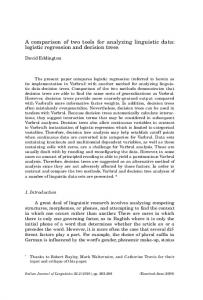
STUDY AREA AND DATASET USED Two datasets were used in this investigation: a Landsat TM scene and field data of the marsh condition. The Landsat TM scene was acquired on November, 11, 1997 and after georectification it was clipped to cover the available field data as shown in Figure 1. The field data is composed of 2,108 data points describing the marsh conditions collected from a low altitude helicopter. The survey (LDWF and USGS, 2001) included information such as latitude, longitude, marsh condition, marsh color, percent vegetated, marsh die-back, and marsh type. The marsh type observations provided information on the water or non-water condition.

Figure 1. Subset of a 1997 Landsat TM scene (p24r39) overlaid with field data representing the study area.

LOGISTIC REGRESSION Logistic regression was used to create simple and accurate models to predict land loss in a repeatable way by allowing the selection of the most appropriate set of independent variables to construct different models. These models were built by combining different independent variables created from spectral band indices (mainly vegetation indices). The outcomes of these models are probability values that a pixel is either water or non-water.

Logistic Regression Overview Logistic regression follows the same principles of linear regression except that the outcome is a dichotomous variable representing success or failure. Often times this is performed by assuming that the probability of success of failure P(X) is related to X by the logit function, which in the case of multiple independent variables can be written as:

P( X ) =

exp(a + β 1 X 1 + β 2 X 2 + ... + βkXk ) 1 + exp(a + β 1 X 1 + β 2 X 2 + ... + βkXk )

Equation 1

where a is the coefficient on the constant term, βk are the coefficients on the independent variables and Xk are the independent variables. In this study the field data was reformatted such that water condition was assigned a value of 1 while the nonwater condition was assigned a value of 0. These values of 1 or 0 are regarded as the dependent variables in the logistic regression modeling that follows.

ASPRS 2007 Annual Conference Tampa, Florida ♦ May 7-11, 2007

Independent Variables Eight variable images were created: Braud Index, IR/R, NDVI, SQRT(IR/R), Vegetation Index, Wetness, Brightness, and Greenness from the tassel cap transform (Wales, 2005). All the variables except the ones from tassel cap were rescaled to eight bit (0-255). A brief description of the reasoning for choosing these spectral indices is presented in Table 1. Table 1. List of the variable images used as independent variables in the logistic regression methodology Spectral Band Ratio

Description

Braud Index

The Braud index is a pseudo-NDVI and it produces high spectral values for water and low spectral values for non-water (Wales, 2005).

IR/R (Band4/Band3)

Water has low spectral response in both Band4 and Band3 while vegetation has a moderate response in Band3 and large response in Band4.

NDVI

Produces high values at vegetated areas due to low reflectance in the visible spectrum and high reflectance in the infrared spectrum (Jensen, 2000).

SQRT(Band4/Band3)

Similar principle as the simple ratio (IR/R) but the square root of the values is used.

VI (Band4 – Band3)

Similar response as the NDVI due to same spectral characteristics of Band4 and Band3.

The “tasseled cap” transformation was originally proposed by Kauth and Thomas (1976) to spectrally highlight important phenomena in the crop development, such as Greenness types of crops, discrimination between crops and background, and soil moisture (Richards and Jia, 1999). As expected wetness yields high values for water and Wetness Brightness and Greenness yield high values for vegetation and low values for water. Summarized from Wales, 2005. Brightness

Model Building and Variables Selection The logistic regression model was set to use the pixel values corresponding to the sensor observation of each variable image as the independent variables and the water (1) and non-water (0) observation from the helicopter survey constituted the dependent variables.

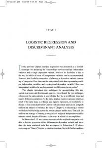
Create model with all predictors

Compute P-Value for each predictor

Does all predictors meet P-value threshold?

Yes

Final model

No Create new model with the predictors that passed the P-Value condition

Figure 2. Simplified flowchart of the stepwise backward elimination process. Variables were individually evaluated based on their level of significance (P-Value associated with Pearson’s Chi-Squared). An iterative process known as stepwise backward elimination was applied to identify and to remove variables that may not be strongly related to the dependent variable or that contain duplicate information provided by other predictors (Devore and Farnum, 1999). Figure 2 shows a simplified flowchart of the stepwise backward elimination process. Variables were removed from the model if their level of significance was greater than 0.10. Initially a model was constructed using all eight independent variables. Braud index was removed because it had a P-Value of 0.916. A second model was build with the seven remaining independent variables and SQRT(IR/R) was also removed with a P-Value of 0.199. In the third iteration, a new model was formed from the six remaining predictors and all independent variables were found to be significant. ASPRS 2007 Annual Conference Tampa, Florida ♦ May 7-11, 2007

The model was applied to the original Landsat image to produce the probability image. Pixel values ranged from zero to one, where zero represents a 0% probability of the pixel being water and a value of one representing a 100% probability of the pixel being water. Using a threshold of 0.5 was possible to convert the probability image into a binary image of water (1) and nonwater (0). This image was compared with the helicopter field data points and the Kappa statistic (Cohen, 1960) was then calculated from the areas with values of one or zeros from the logistic regression model when compared to the 1 and 0 values from the field helicopter transects. Kappa statistics was selected as accuracy measure between the predicted and observed categorized data because it allows correction of agreement due to chance. The Kappa coefficient of agreement was 0.7186 for the selected model. For a more detailed description of the logistic regression procedure to quantify and to predict Coastal Louisiana land loss please refer to Wales (2005).

GENETIC PROGRAMMING Genetic programming was used as an optimization tool to generate functions, composed of spectral indices and spectral transformation, to map the original image into a classified image (binary domain) of the desired feature (water, as previously described). The inputs were: a LANDSAT scene (same scene used in the logistic regression approach) and the helicopter field data used in the training process.

Genetic Programming Overview GP was first introduced by Koza (1992) to solve problems from different domains. The main goal is to solve these problems by searching a space of possible computer programs for any program (usually the most fit), among all possible programs, that solves the problem (or approximately solves it). This simulated evolutionary characteristic of GP is often referred as an optimization algorithm because it uses a combinatorial search approach that is capable of automatically deriving code which proceeds by trial and error repetition. GP differs from genetic algorithms and other machine learning algorithms in its hypothesis representation. In GP the hypotheses are computer programs represented in a hierarchical tree structures rather than a set of rules represented by different types of structures (such as fixed size strings or weight vectors) commonly used by other machine learning algorithms. GP’s main components are: a set of functions (the building blocks for the computer programs), a set of parameters (the arguments to be used by the computer programs) and a fitness function designed to provide the means to compare and to rank the set of candidate hypothesis. GP operates in an iterative mode by constantly updating the set of candidate hypotheses (also known as the population) until the most fit hypothesis (individual) is found. Initially, the first population is randomly generated and after each iteration (generation), the set of hypotheses are evaluated based on the fitness function and sorted accordingly. Hypotheses with the highest fitness values are then selected to be carried forward to the next set of hypotheses (or new generation). Some of the hypotheses are carried forward with no change (replication) while others are susceptible to genetic operations such as crossover, and mutation. The crossover operation produces two new individuals from the parents by copying parts from each parent, while the mutation operation produces small random changes to small parts of the individual. When the stopping criteria are met the process comes to an end and the most fit individual is the result.

⎛ ⎝

log ( B5) ⎛ B1 ⋅ 2 ⋅ B5 ⎞ + B6⎞ > ⎝ 123.336 ⎠ ⎠ ABS( B5 − 248.339)

log⎜ log ⎜

A

Equation 2

B

Overall Framework The framework was established to use the helicopter field data as the “truth” data duringin the training process. The genetic programming parameters used are shown in Table 2. Some of the functions were modified to avoid unwanted situations such as division by zero and complex numbers. The spectral band values were considered as variables (B1-B6) were the digital numbers of the pixels containing the field data points. The fitness of each candidate spectral function was calculated by applying each of them individually and then computing the accuracy using the Kappa statistic (Cohen, 1960).


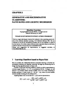
Equation 2 shows the final spectral function, after simplification. In Equation 2 if term A is greater than term B the algorithm assigns zero (non-water) otherwise it assigns one (water). A Kappa statistic of 0.7394 was obtained by this method. Figure 3 shows the final classified image from the genetic programming approach. Table 2. Genetic Programming parameters used Terminal set

Variables: B1,B2,B3,B4,B5,B6 (LANDSAT 7 ETM+ spectral bands) Constants: 0 to 255 (representing the possible digital number values)

Function set

SUM, SUB, DIV , SQRT , LOG , ABS, Wrapper (if a>b then 0 else 1)

Population size

500

Number of generations

51 (initial plus 50 new)

Percentage of cross-over

30%

1

2

3

1 - safe division, 2 - safe square root, 3 - safe logarithm

Figure 3. Result classified image from the genetic programming methodology.

LOGISTIC REGRESSION AND GENETIC PROGRAMMING INTEGRATED Both of the previously described methods have demonstrated results with similar Kappa values (0.7186 and 0.7394) indicating good agreement, as suggested by Lands and Kock (1977). However there are some complementary characteristics of these methods that justify the investigation of a third approach of integrating them to further improve the modeling capabilities. Some of these characteristics include: Logistic regression: • Provides the tools to quantify the significance of each predictor in the model and therefore screens for the most significant predictors. • Standard method of analysis when the outcome variable is dichotomous. • Generates a probability image with the probability of membership of each pixel. • The work of Wales (2005) has shown that the models are not scene specific and therefore they can be developed in one scene and applied to another with reasonable results. Genetic programming: • Due to its optimization characteristics can develop new feature-specific spectral indices and transformations. • Works with incomplete or missing data. • Robust classification capabilities when compared with other classification algorithms, including artificial neural network, support vector machine, and others (Daida et al.,1996). • Ability to generate different types of codes, from scripts to assemble improving this way its integration ability with existing commercial imagery processing software.


Vinterbo and Ohno-Machado (1999) have investigated the use of the genetic algorithms to select variables from a dataset with a fixed number of variables to construct logistic regression models. Their work compared these models with models constructed using standard forward, backward and stepwise variable selection procedures. In the current research, the independent variables are spectral indices derived from the image spectral bands and therefore we do not have prior knowledge of either of the number of predictors to use nor of their form (spectral indices are not previously defined). Therefore the objective of this research is to use genetic programming as an optimization tool to determine the number and type of spectral indices to be used as independent variables of the logistic regression approach. More than 20 vegetation indices are currently in use (Jensen, 2000 and Lillesand and Kiefer, 2000). These vegetation indices were designed to address specific problems by using information from specific sensors, and therefore the selection of the proper spectral index can be viewed from an optimization stand point.

Fitness Measurement Since different models will be compared with each other it is important to define a quantitative measure of performance to select the most appropriate model. Models can be compared in terms of performance (discriminatory ability), robustness (generalization ability), and explanatory power (Vinterbo and Ohno-Machado, 1999). Additionally, a smaller and simpler model is desired because it is easier to explain, it cost less (in terms of computational effort), and avoids over-fitting improving this way the chances of generalization. Herein we have concentrated our efforts to maximize the performance while keeping the model simple (valuing smaller number of terms), thus our fitness function is mathematically expressed by:

⎛ vi − Nv ⎞ f ( Mi, DV ) = Kappa + ρ * ⎜ ⎟ ⎝ Nv ⎠

Equation 3

where: Mi is the model being evaluated DV is the dependent variable dataset Kappa is a coefficient that measures the accuracy of classification corrected for agreement due to chance proposed by Cohen (1960) ρ is the weight vi is the number of predictors considered in the model being evaluated Nv is the maximum number of predictors allowed Equation 3 will provide a high fitness value for models with a high Kappa values and a small number of predictors. The weight coefficient ρ is designed to allow different rewards standards for the number of predictors.

R SUM

DIF

32

DIV

SQRT

B1

Predictor 1 (32 - B1) + (SQRT(B1))

MUL

MUL

B1

B5

SUM

B3

B4

SUM

B1

Predictor 2 (B5 * B3) / (B4 + B1)

B5

LOG

51

B5

Predictor N (B5 + 51) * (LOG(B5))

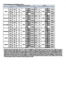
Figure 4. Example of a proposed candidate model representation for the genetic programming and logistic regression integrated method.


Overall Framework Description In genetic programming each of the candidate solutions is represented in a hierarchical tree structure. This structure is composed of: functions and terminals. Functions are the nodes of the tree and they can be of two different types: binary (takes two arguments, such as summation and multiplication) or unary (takes one argument, such as logarithm and square root). Terminals can be seen as the leaves of the tree or in other words the arguments used by the functions. Three examples of the genetic programming hypothesis representation are displayed in the dashed boxes of Figure 4. In this proposed methodology, a new type of node will be considered, the root node (the note outside of the dashed boxes in Figure 4). The root node will not have a fixed number of branches, as the binary (two) and unary (one) nodes, but rather it will vary according to a user-defined range. Each branch represents one independent variable (in the form of a spectral index). Random create candidate models 1

Stepwise backward elimination 2

Original Image

3

Create revised models

4

For each model compute fitness

Genetic operations 7 5

GP parameters

Yes

No 6

Sort models by fitness

Stopping criteria

Final model

Figure 5. Simplified flowchart of the genetic programming and logistic regression integrated methodology. The genetic programming parameters considered are the same ones considered for the genetic programming methodology, except that the function set is extended to incorporate convolution functions with pre-defied kernel sizes such as 3x3, 5x5, and 7x7. The convolution functions considered were mean and standard deviation. The flowchart for the proposed methodology is shown in Figure 5. In the first step a set of candidate models (hierarchical tree structure as shown in Figure 4) is randomly generated. Each of the candidate models generated has a different number of predictors and each of the predictors (spectral indices) is also different from the others since they were randomly selected by the genetic programming algorithm. A standard stepwise backward elimination process is then applied to all P candidate models to eliminate predictors that do not bring significant information to the model by using as threshold the P-Value associated with Pearson’s Chi-Squared of 0.10. A new set of revised candidate models are then produced using only the predictors that passed the level of significance test. In step four the fitness value of each candidate model is then computed using Equation 3. In step five the algorithm stopping criteria are evaluated. The stopping criteria are defined as either the maximum number of iterations or a fitness threshold. If either one of the stopping criteria is met then the final model (the most fit one) is output, otherwise the set of candidate models are then sorted by fitness values (step 6). Genetic operations are then performed and a new set of candidate models is formed with the most fit models. The entire process is then repeated until one of the stopping criteria is met.

DISCUSSION The proposed methodology is part of an ongoing research designed to establish a standard procedure to be incorporated into a decision support system (DSS) designed to monitor and to quantify the Coastal Louisiana land loss over time. One of the requirements of the DSS is simplicity. Even though the methods described in this manuscript can be considered complex, these steps are intended only to investigate the most appropriate methodology (model), which will then be included in the DSS to be used on an operational basis. The genetic programming optimization characteristic has demonstrated its value in the creation of new spectral indices and transformations in a problem specific fashion. However, the presence of the threshold function (also known as wrapper) constitutes a threat to the model’s generalization ability. For instance, there are two constants ASPRS 2007 Annual Conference Tampa, Florida ♦ May 7-11, 2007

(123.336 and 248.339) in Equation 3 were developed specifically for this LANDSAT scene and they may not be the most appropriate for another scene. Conversely, the logistic regression approach has shown significant value through the work of Wales (2005). The only draw back in this methodology is the selection of the independent variables (spectral indices). The Coastal Louisiana land loss is a complex problem where water and land must be delineated from each other in an environment where water, soil, and vegetation are mixed together and therefore the selection of the appropriate spectral index constitutes a challenge. The proposed integrated genetic programming and logistic regression methodology should enhance the modeling by using the complementary characteristics of each individual method: logistic regression ability to produce robust models with statistical measures of each predictor and the genetic programming optimization characteristics of searching the most appropriate solution among the space of possible solutions.

FUTURE WORK As part of an ongoing research there are important issues that still need to be addressed. After focusing on the performance of the models it will be necessary to investigate their generalization ability by evaluating them on images with different spatial location and temporal variation. Additionally, it may be necessary to investigate remote sensing parameters such as spatial and spectral resolution since it may be necessary to use a multi-sensor approach.

ACKNOWLEDGEMENTS The authors would like to acknowledge the University of Mississippi Geoinformatics Center (UMGC) for providing the financial support and the access to the computer infrastructure made available at the University of Mississippi. We also would like to thank Mr. Wales for sharing the field data as well as his finding.

REFERENCES Cohen, J. (1960). A coefficient of agreement for nominal scales. Educational and Psychological Measurement, 20(1): 37-46. Daida, J.M., T. F. Bersano-Begey, J. S. Ross, and J. F. Vesecky (1996). Evolving Feature-Extraction Algorithm: Adapting Genetic Programming for Image Analysis in Geoscience and Remote Sensing, Proceedings of the International Geoscience and Remote Sensing for a Sustainable Future, Washington, USA. Devore, J. and N. Farnum (1999). Applied Statistics for Engineering and Scientists. Duxbury Press, USA. Jensen, J.R. (2000). Remote sensing of the environment: an earth resource perspective. Prentice-Hall, USA. Kauth, R., J. and G. S. Thomas (1976). The Tasseled Cap - A Graphic Description of the Spectral-Temporal Development of Agricultural Crops as Seen by Landsat, Proceedings of LARS - Symp. on Machine Process: Remotely Sensed Data, Purdue University, USA. Koza, J.R. (1992). Genetic Programming - On the programming of computers by means of natural selection. Massachusetts Institute of Technology, USA. Landis, J.R. and G. G. Kock (1977). The Measurement of observer agreement for categorical data. Biometrics, Vol 33, No 1, pp 159-174. LDWF and USGC (2001). 2001 Louisiana coastal marsh vegetative type transect point database., Louisiana Department of Wildlife and Fisheries (LDWF), Fur and Refuge Division, and United States Geologic Survey (USGS), Biological Resources Division National Wetlands Research Center (NWRC), Lafayette, LA, USA. Lillesand, T.M. and R. W. Kiefer (2000). Remote Sensing and Image Interpretation. John Wiley & Sons, Inc., USA. Richards, J.A. and X. Jia (1999). Remote Sensing Digital Image Analysis. Springer, Berlin, Germany. Vinterbo, A., and L. Ohno-Machado (1999). A genetic algorithm to select variables in logistic regression: example in the domain of myocardial infarction. Journal of the American Medical Informatics Association, (6): 984988. Wales, P.M. (2005). Quantitative Analysis of Land Loss in Coastal Louisiana Using Remote Sensing. Master of Science Thesis, The University of Mississippi, University, MS, USA. ASPRS 2007 Annual Conference Tampa, Florida ♦ May 7-11, 2007