Proceedings of the 2003 IEEE/RSJ Intl. Conference on Intelligent Robots and Systems Las Vegas, Nevada · October 2003
Interactive-Motion Control of Modular Reconfigurable Manipulators Weihai Chen*
Guilin Yang*
Edwin Hui Leong Ho*
I-Ming Chen+
*
Singapore Institute of Manufacturing Technology 71 Nanyang Drive, Singapore 638075
whchen, glyang,
[email protected]
[email protected]
+
School of Mechanical & Production Engineering Nanyang Technological University, Singapore 639798 ABSTRACT ─ A joystick-based interactive motion control approach is proposed for modular reconfigurable manipulators. Based on the product-of-exponentials (POE) formula, the velocity models as well as the incremental displacement models have been formulated for both serial manipulators (with arbitrary configurations and DOFs) and a class of three-legged parallel manipulators. As a result, two different control modes, i.e., the velocity control mode and the incremental displacement control mode, have been developed. A user-friendly GUI has also been developed, which can display the joystick input, the actual joint angles, and the end-effector pose simultaneously. The effectiveness of this approach has been demonstrated by a 6-DOF serial modular robot and a 6-DOF 3RPRS parallel robot.
1
Introduction
A modular reconfigurable robot system consists of a collection of robot modules such as actuators, rigid links, and end-effectors [1, 2, 3]. These modular components can be rapidly assembled into various robot configurations having different working capabilities [4, 5]. However, the formalization of a generalized control scheme for such a modular manipulator is more difficult than a conventional manipulator due to its flexibility in configuration [6, 7, 8]. Hence, “teach and play back” is an effective and convenient way for the motion control of a modular manipulator. In this circumstance, a joystick can be employed as an intuitive position or velocity input device. It makes interactive communication between operator and robot possible, which is an important feature of intelligent robots [9]. Moreover, the algorithms developed for the joystick-based motion control can be readily extended to the haptic device-based tele-presence control [10, 11, 12]. A joystick-based motion control can be realized in either joint space or Cartesian space. Obviously, the joint-space motion control is easy and straightforward. It does not need kinematics models so that it is independent of manipulator configurations. However, the major drawback of the joint-space motion control lies in that the operator has no feeling about the end-effector motions in Cartesian space. Hence, accurate position controls in Cartesian space are unable to achieve. In this paper, we will mainly focus on the joystick-based 0-7803-7860-1/03/$17.00 © 2003 IEEE
Cartesian space motion control. Because the joystick motion is quite flimsy, absolute position control will easily result in jerky motions of the manipulators. Instead, two kinds of stable control modes, i.e., velocity control mode and incremental displacement control mode have been proposed. In general, the incremental displacement control can achieve higher positioning accuracy than the velocity control. On the other hand, the velocity control can enable the manipulator to move more smoothly than the incremental displacement control. Since a modular reconfigurable robot can assume any possible manipulator configurations, both serial and parallel manipulators need to be considered. For the serial manipulators, there are no configuration limitations. For the parallel manipulators, however, because of the complexity of their configuration types, a class of three-legged manipulators is selected as the norm of modular parallel manipulators [13]. In order to realize the Cartesian-space motion control, it is essential to formulate the kinematic models for both serial manipulators and the three-legged parallel manipulators. Based on the POE formula, both the instantaneous kinematics models and the incremental displacement models have been formulated. With the proposed kinematic algorithms, a user-friendly GUI has been developed using VC++. By retrieving the data from both joysticks output ports and the manipulator’s joint modules, the GUI can display the control mode, the joystick input, the actual joint angles, and the actual end-effector pose simultaneously. In brief, such a joystick-based motion control method provides the end-user an easy-to-access, interactive and efficient control interface for modular reconfigurable robots.
2
Modular Reconfigurable Robot System
A modular reconfigurable robot system consists of a series of standard active-joint modules, passive-joint modules, and customized rigid links and end-effectors that can be assembled into a variety of robot configurations. The active-joint module is a self-contained compact mechatronic drive unit with the built-in motor, encoder, controller, amplifier, harmonic drive, and communication interface. The active-joints modules are 1-DOF revolute joint modules, 1-DOF prismatic joint modules, and 2-DOF wrist joint modules. The passive joint modules are basically rotary joint modules, universal joint modules and spherical
1620
joint modules. Some of the active- and passive-joint modules are shown in Figure 1(a) and (b), respectively.
where ωˆ i ∈ so(3) is a skew-symmetric matrix related to
ω i ∈ R 3×1 which is the unit directional vector of the joint axis i expressed in frame i, υ i ∈ R 3×1 is the position vector of the joint axis i expressed in frame i. The twist sˆi can be expressed as a 6 by 1 vector s i through a mapping
(a) Active-joint modules
(b) Passive-joint modules
Fig. 1 Robot modules With an inventory of such robot modules, various robot configurations can be rapidly constructed. A 6-DOF serial modular manipulator and a 6-DOF 3RPRS parallel modular manipulator are illustrated in Fig. 2 (a) and (b), respectively.
sˆi a si = (υi ,ωi ) ∈ R6×1 , where s i is the twist coordinate of joint axis i. Therefore, based on the dyad kinematics (Eq.(1)), the forward kinematics of a serial open chain robot with n joints can be expressed as T0, n (q1 ,q 2 ,L ,q n ) = T0,1 (q1 )T1, 2 (q 2 ) L Tn −1,n (q n ) (3) ˆ ˆ ˆ = T0,1 (0)e s1q1 T1, 2 (0)e s2 q2 L Tn −1, n (0)e sn qn
3.2 Velocity analysis
The end-effector pose, T0, n, can also be written as: R T 0, n = 0,n 0
p 0, n , 1
(4)
where R0,n ∈ SO (3) and p 0,n ∈ R 3×1 are the orientation
(a)
Serial type Fig. 2
3
matrix and the position vector of frame n (end-effector) with respect to frame 0 (base), respectively. Hence, we have R& R T − R& 0, n R0T, n p0, n + p& 0, n , (5) T&0, nT0−, 1n = 0, n 0, n 0 0 where T& 0 , nT 0−, n1 ∈ se (3) is termed the spatial velocity of the
(b) Parallel type
Modular manipulators
end-effector frame n with respect to the base frame 0 [14], ) denoted by V 0s, n which can be given by
Kinematics for Serial Manipulators
ωˆ s Vˆ0s, n = 0 , n 0
3.1 Product of exponentials formula Let link i-1 and link i be two adjacent links (termed a dyad) connected by joint i, as shown in Fig. 3 [5]. si
yi -1 i-2 nk Li
xi -1
i -1
link i -1
yi
i
(7)
where the angular component, ω 0s, n , is the instantaneous angular velocity of the body as viewed in the spatial (base) frame; the linear component, υ0s, n , is the velocity of a
Link i and joint i are termed link assembly i. If we denote the body coordinate frame on link assembly i by frame i, the relative pose of frame i with respect to frame i-1, under a joint angle displacement, q i , can be described by a 4 by 4 homogeneous matrix, such that ,
)
the twist coordinates of the spatial velocity V 0s, n , i.e.,
link i
Fig. 3 Two adjacent links - a dyad
Ti −1,i (q i ) = Ti −1,i (0)e
(6)
υ s − ω 0s, n × p 0 , n + p& 0 , n V 0s, n = 0s, n = , ( R& 0 , n R 0T, n ) ∨ ω 0 , n
xi
sˆi qi
0
V0s, n ∈ R 6×1 can be written as:
zi
zi -1
υ 0s, n ,
(possibly imaginary) point on the same rigid body which is traveling through the origin of the spatial frame [14]. Based on Eq.(3), Eq.(7) can also be written as (8) V0s, n = J 0s, n (q ) q& , where J 0s,n (q) = [(
(1)
where Ti −1,i (0) ∈ SE (3) is the initial pose of frame i w.r.t frame i-1, qi ∈ R is the joint angle, and sˆi ∈ se(3) refers to the twist of joint axis i (expressed in frame i). It has the form of vi ωˆ , (2) sˆ i = i 0 0
∂T0, n −1 ∨ T ) ∂q1 0, n
L (
∂T0, n −1 ∨ T ) ]. ∂qn 0, n
(9)
The matrix J 0s, n ( q ) ∈ R 6 × n is termed as the spatial manipulator Jocobian Matrix [14]. It’s ith column can be written as ∂T0 , n (10) T0−, n1 = T 0, i sˆ i Ti , n T0−, n1 = T0 , i sˆ i T0−, 1i , ∂q i
Converting it into twist coordinates, we have
1621
(
∂T0 , n ∂qi
T0−, n1 ) ∨ = Ad T0 , i s i ,
(11)
where Ad T s i is termed as the Adjoint Representation of 0, i T0,n [14].
leg is a 6-DOF serial kinematic chain with two actuators, as shown in Fig. 4. To further simplify the kinematic structure, a 3-DOF passive spherical joint is placed at each of the A leg-ends. 3
z
A1
As described earlier, the spatial velocity of the end-effector is different from the conventional expression of the end-effector velocity, which makes it difficult to be implemented to intuitive motion control. The natural and conventional way to represent the end-effector velocity has the form of
where ( J 0h, n ) + is the pseudoinverse of J 0h, n 3.2 Incremental displacement analysis
Although the velocity control mode can generate smooth motions, its control accuracy is not high enough. When a robot moves close to its target position, the incremental displacement control mode need to be employed so as to satisfy the accuracy requirement. Define the (hybrid) incremental displacement of a rigid body as δ p 0 , n (15) δD 0h, n = s , δθ 0, n
33
z
x
B 32
z
x
y
y
x
B 12
s^32
y
y z
B 23
s^31
x
y
s^11
x x z
y
B 11 (B 10 )
B
B 31 (B 30 )
y
s^22 B 22
z y
x z
s^21 y
x
B 21 (B 20 )
Fig. 4 A three-legged 6-DOF parallel manipulator 4.1 Forward displacement analysis
For each of the legs, assume that the first two joints are active joints and the third one is a passive revolute joint module in which an incremental encoder is installed to measure its joint displacement. The purpose of the forward displacement analysis is to determine the end-effector poses with given active-joint angles. Define frame A as the local frame attached to the mobile platform, frame B as the base frame, and point Ai (i = 1, 2, 3) as the center of the spherical joint coupling the leg with the mobile platform. As shown in Fig. 4, if the coordinates of the point Ai with respect to frame A and frame Bi ,3 are given by p ia = ( x aia , y aia , z aia ) T and pai ′ = ( xai ′ , y ai ′ , z ai ′ )T , respectively, the forward kinematics of the three-legged parallel robots can be given by [15] −1
where the vector δp0,n = [δp( 0,n ) , δp( 0,n ) , δp(0,n ) ]T ∈ R 3×1 x y z
TB, A
and δθ 0,n = [δθ ( 0,n ) , δθ ( 0,n ) , δθ ( 0,n ) ]T ∈ R 3×1 represent the x y z incremental position and orientation vectors of the end-effector with respect to the base, respectively. Based on the definition of hybrid velocity as well as Eq.(15), the relationship between the incremental joint angles and the hybrid incremental displacement can be given by (16) dq = ( J 0h,n ) + δD0h,n ,
s^
s^23
−1
3×3
B 33
x
x
z
s^12
where p& 0, n represents the linear velocity and ω 0s,n represents the angular velocity. Both are viewed in the base frame. Such a velocity is also termed as the hybrid velocity of a rigid body [14]. Thus, according to Eqs. (7) and (12), Eq.(8) can be rewritten as (13) V0h,n = J 0h,n q& ,
x
A2
z
Jocobian matrix of the manipulator. Hence, the joint velocity can be given by (14) q& = ( J 0h, n ) + V0h,n ,
y
B 13
(12)
ˆ where J0h,n = I3×3 p0,n J0s,n∈ R6×n represents the hybrid 0 I
A
y
z
V 0h, n
p& 0 , n = s , ω 0 , n
s^13
z
a a p p p p × p23 p1a p2a p3a p12 × p23 = 1 2 3 12 , 0 1 1 1 0 1 1 1
(17)
where the positional vector of the point Ai is written as pi p′ ˆ ˆ sˆi1qi1 TBi1 , Bi 2 (0)e si 2qi 2 TBi 2 , Bi 3 (0)e si 3qi 3 i . 1 = TB, Bi1 (0)e 1 (18) In Eq.(18), sˆij ∈ se (3) (i = 1, 2, 3; j = 1, 2 ) is the twist of
where dq = [dq1, dq2, L, dqn ]T∈ Rn×1 represents the joint angle incremental vector.
a a joint axis ij expressed in frame ij; p12 = p2a − p1a , p23 = p3a − p2a and p12 = p2 − p1 , p23 = p3 − p2 .
4
4.2 Velocity analysis
Kinematics for Parallel Manipulators
A class of three-legged 6-DOF modular parallel manipulator is the subject of this Section. Considering the symmetrical design, each leg is identical to the others. In addition, each
The objective of velocity analysis is to determine the relationship between the six active-joint rates and the velocity of mobile platform. The twist annihilator method
1622
proposed in [16] is employed here for the formulation of the velocity model. Differentiating both side of Eq.(18) with respect to time, we can obtain p& i p i′1, i p i′2 , i 0 = T B , B i 1 sˆ i1 1 q& i1 + T B , B i 2 sˆ i 2 1 q& i 2 ′ p + T B , B i 3 sˆ i 3 i 3 , i q& i 3 , i = 1, 2 , 3 , 1
active–joint rate, q& a , can be written as J a q& a = J f V Bs, A ,
where
ˆ
TB , Bi 2 = TB , Bi1 (0)e TB , Bi 2 = TB , Bi1 (0)e
sˆi1qi1
TBi1 , Bi 2 (0)e
sˆi 2 qi 2 ˆ
ˆ
TBi1 , Bi 2 (0)e si 2 qi 2 TBi 2 , Bi 3 (0)e si 3qi 3 . (20)
pij′ ,i ∈ R 3×1 (with pi′3,i = pi′ ) is the position vector of point pi′1,i = TBi1 , Bi 2 (0)e
pi′2,i = TBi 2 , Bi 3 (0)e
TBi 2 , Bi 3 (0)e
sˆi 3 qi 3
sˆi 3 qi 3
.
(30)
f
(u 12 × u 13 ) T T P 1 T (u 13 × u 11 ) T P1 (u × u ) T T 22 23 P2 ∈ R 6× 6 = (u 23 × u 21 ) T T P 2 T (u 32 × u 33 ) T P3 , (u × u ) T T 31 P3 33
(31)
j a11 = (u 22 × u 23 ) T u 21 ,
j a 22 = (u 23 × u 21 ) T u 22
j a11 = (u 32 × u 33 ) T u 31 ,
j a 22 = (u 33 × u 31 ) T u 32
Introducing hybrid velocity concept to Eq.(28), we have I J a q& a = J f 3× 3 0
(21)
Let RB,Bij ∈ SO(3) be the orientation matrix of TB , Bij , sij is the twist coordinates of joint ij expressed in frame ij, and TPij′,i = [I3×3 − pˆij′ ,i ] , where pˆ ij′ ,i ∈ R 3×3 is the skew symmetric (cross-product) matrix related to vector p ij′ ,i ∈ R 3×1 . Hence, Eq.(19) can be simplified as [15] p& i = u i1 q& i1 + u i 2 q& i 2 + u i1 q& i 3 , i = 1, 2, 3
q&a = [q&11, q&12 , q&21, q&22 , q&31, q&32 ]T ,
with the notations below: j a11 = (u12 × u13 ) T u11 , j a 22 = (u13 × u11 ) T u12
Ai with respect to frame ij, which is given by sˆi 2 qi 2
(29)
J
is the forward kinematic transformation of frame ij with respect to frame B, which is given by sˆi1qi1
J a = diag[ j a11 j a22 j a33 j a44 j a55 j a66 ] ,
(19)
where q& ij (i = 1, 2, 3; j = 1, 2, 3) is the rate of joint ij, TB , Bij
TB , Bi1 = TB , Bi1 (0)e si1qi1
(28)
pˆ B , A h V B , A , I 3× 3
where p B , A ∈ R 3×1 is the position vector of the forward kinematics TB , A , and VBh, A = [ p& B , A , ω B , A ]∈ R 6×1 is the hybrid velocity of the mobile-platform frame A. Define manipulator forward hybrid Jacobian matrix as J h , we have J a q& a = J hV Bh, A ,
(22)
q& i1 (u i 2 × u i 3 ) T u i1 = (u i 2 × u i 3 ) T p& i . (23) )s Let V B , A represents the spatial velocity of the mobile
platform, which can be computed as p& i ˆ s pi TPi υ Bs , A (24) 0 = VB , A 1 = 0 s , i = 1, 2, 3 ω B, A where TPi = [I 3×3 − pˆ i′ ] . Let VBs, A = [υBs , A , ωBs , A ] . Then we have p& i = TPi V Bs, A
(25)
Substituting Eq.(25) into Eq.(23), we have q& i1 (u i 2 × u i 3 ) T u i1 = (u i 2 × u i 3 ) T TPi V Bs, A .
(26)
Following a similar procedure, we have q&i 2 (ui 3 × ui1 )T ui 2 = (ui 3 × ui1 )T TPi VBs, A .
(27)
Hence, the instantaneous kinematic relationship between the mobile platform twist coordinate, VBs, A , and the
(33)
where
where uij = RB, Bij TPij′ ,i sij . Since we are interested in the relationship between the active-joint rates and the mobile-platform velocity, the passive-joint rates should be eliminated from Eq.(22). To this end, we dot-multiply both sides of Eq.(22) by twist annihilator u i 2 × u i 3 to get joint rate q& i1 . We have
(32)
I J h = J f 3×3 0
pˆ B , A . I 3×3
(34)
If the inverse kinematic matrix, J a , is nonsingular, then the active-joint rate vector, q& a , is given by q& a = J a−1 J hV Bh, A
(35)
4.3 Incremental displacement analysis
Similar to the serial manipulators, the relationship between the incremental joint angles and the hybrid incremental displacement can be given by dq a = J a−1 J h δD Bh , A (36)
where dqa = [dqa1, dqa2 , L, dqa6 ]T∈ R6×1 represents the active-joint angle incremental vector, and δD Bh , A ∈ R 6×1 represents the incremental position and orientation vector of the mobile-platform frame A with respect to the frame B. 5
Joystick Output Data
A WingMan Extreme™ Digital 3D joystick is employed as a motion input device, as shown in Figure 5. This joystick has seven programmable buttons and four controllable axes through operating the stick handle and a
1623
throttle. The stick handle has three DOFs such as the left-right motion (LRmove), forward-backward motion (FBmove), and twist motion (Twist). For Cartesian space control, LRmove, FBmove, and Twist are used to control the manipulate motion (translation and rotation) about X, Y, and Z-axis, respectively. For joint space control, only the forward-backward motion of the stick handle will be used to control the selected joint. The throttle is used to perform fine step control because it can capture small input Button 1
Button 4
Button 2
Button 5 Handle
Button 3
6
FBmove LRmove
Experimental Studies
6.1 A 6-DOF serial manipulator
Twist
A 6-DOF serial manipulator as shown in Fig. 2 (a) is used to verify the velocity control mode. Choose appropriate mapping factors to let the end-effector of the manipulator have maximum velocity 160deg/sec. Using the forward kinematics algorithm, the initial pose of the end-effector is
Button 6 Button 7 Throttle
Fig. 5
displayed in Axis Chosen box can be sequentially changed by pressing joystick button 1 and 2 (in either ascending or descending orders). The control mode (velocity control or incremental displacement control) can be switched by pressing joystick button 7 (Fig. 5), and the message shown the control mode is displayed in Status box that is located in the left area of part four. The Status box also displays other messages such as Initializing, Reset, Halt etc. Joystick messages from USB interface of PC is periodically inquired through setting a timer. The enquiry can be responded by VC++ system structure function DIJOYSTATE defined in the head file dinput.h.
WingMan extreme digital 3D joystick
A joystick control interface is illustrated in Fig. 6. This interface contains four parts. Part one displays the actual end-effector pose and joint angles. Part two has two columns. The left column is designed for the joint space control, which displays joint rates (or joint angle increments). The right column is used for Cartesian space control, which displays the end-effector’s velocity (or displacement increments). Part three displays joystick value. Part four is used to choose the control types and modes.
1 0 0 0
0 0 −1 0
0 − 325 225 1 .
(37) Now let us control the end-effector to move in -X direction. First, select the control type in the Axis Chosen box to be X. Then, move the stick handle of the joystick towards right direction with velocity about 50mm/sec till the position output value of X axis shown in the interface to be -160mm. As expected, the end-effector of the manipulator moved along the negative X-axis direction to the desired point (Figure 7)
Part II
Part III
Part I
0 1 T [0] = 0 0
Fig. 7
6.2 Parallel robot experiment
Part IV
Fig. 6
Move along X-axis positive direction
A 6-DOF 3RPRS parallel manipulator as shown in Fig. 2 (b) is used to verify both the velocity and incremental displacement control modes. The manipulator has initial pose as R = I and P = [0, 0, 609]T
The interface of joystick control
There are two kinds of control types, namely joint space or Cartesian space. The control type can be switched by pressing joystick button 6 (Fig 5). Furthermore, the joint number displayed in Joint Chosen box and the axis symbol
• Translation along Z-axis Select the control type in the Axis Chosen box to be Z. Then, rotate the stick handle of the joystick in clockwise direction with a velocity about 50mm/sec so as to move the
1624
end-effector along the negative direction of Z-axis. When the end-effector is closed to the target location (Z=370mm), the control mode is switched to incremental displacement control mode with 0.1mm resolution. This straight-line control is illustrated in Fig. 8.
Fig. 8
Robot at working location
• Rotation about X-axis Select the control type in the Axis Chosen box to be Rx. Then, move the stick handle of the joystick towards left side with a velocity about 0.1rad/sec to rotate the end-effector around the positive direction of X-axis. When the end-effector is closed to the target orientation ( θ x = 0.4363rad or 25degree), the control mode is switched
to incremental displacement control with angular increment 0.01rad. This rotation control is illustrated in Fig. 9.
Fig. 9 Rotate about X-axis positive direction
7
Summary
In this paper, a joystick-based interactive motion control interface has been developed for modular reconfigurable manipulators. The kinematics models and algorithms are formulated based on POE formula, which are suitable for both serial and parallel manipulators. Two different control modes, namely velocity control mode and incremental displacement control mode, have been proposed. The velocity control mode can achieve faster and smoother manipulator motion so that it can be employed for coarse motion control. The incremental displacement control, on the other hand, is mainly used for high-resolution step motion control. By combining these two different control modes sequentially, a fast, smooth, and precision motion control can be achieved. The effectiveness of this intuitive and interactive control approach has been experimentally demonstrated.
Acknowledgment This work is supported by Singapore Institute of Manufacturing Technology under the applied research project grant C01-A-137-AR and the university collaboration project grant U97-A-006.
References [1] G. L., Yang, W. H. Chen, and I. M. Chen, “A Geometrical Method for the Singularity Analysis of 3-RRR Planar Parallel Robots with Different Actuation Schemes” in Proceedings of IEEE/RSJ Inter. Conf. of Intelligent Robots and Systems, Lausanne, Switzerland, Sept. 2002, pp.2055-2060 [2] C. J. J. Paredis, “An Agent-Based Approach to the Design of Rapidly Deployable Fault Tolerant Manipulators,” PhD Dissertation, Carnegie Mellon University, USA, 1996 [3] I. M. Chen, S. H. Yeo, G. Chen, and G. L. Yang, "Kernel for Modular Robot Applications – Automatic Modeling Techniques", Inter. Journal of Robotics Research, 18(2), 1999, pp. 225-242 [4] G. L., Yang, W. H. Chen, and H. L. Ho, “Design and Kinematic Analysis of a Modular and Hybrid Parallel Serial Manipulator”, Proc. of 7th Int. Conf. on Control, Automation, Robotic and Vision, Singapore, Dec. 2002, pp.45-.50 [5] I. M. Chen, and G. L. Yang, “Inverse Kinematics for Modular Reconfigurable Robots,” in Proc. of IEEE Inter. Conf. on Robotics and Automation, 1998, pp. 1647-1652 [6] F. C. Park, "Computational Aspect of Manipulators via Product of Exponential Formula for Robot Kinematics," IEEE Trans. on Automatic Control, 39(9): 1994, pp. 643-647 [7] J. Z. Xiao, H. Dulimarta, N. Xi, R. L. Tummala, “Motion Planning of a Bipedal Miniature Crawling Robot in Hybrid Configuration Space”, in Proceedings of IEEE/RSJ Inter. Conference of Intelligent Robots and Systems, Lausanne, Switzerland, Sept. 2002, pp.2407-2412 [8] W. H. Chen, G. L. Yang, and K. M. Goh, “Kinematic Control for Fault-Tolerant Modular Robots Based on Joint Angle Increment Redistribution” Proc. of 7th Inter. Conf. on Control, Automation, Robotic and Vision, Dec. 2002, pp.396-401 [9] T. Fong , I. Nourbakhsh, and K. Dautenhahn, “A survey of socially interactive robots”, Robotics and Autonomous Systems, 42, 2003, pp. 143–166 [10] N. Turro, O. Khatib., E. Coste-Maniere, “Haptically Augmented Teleopration”, in Proc. of IEEE Inter. Conf. on Robotics and Automation, Korea, May 2001, pp.386-392 [11] J. M. Hollerbach, "Some Current Issues in Haptics Research", in Proceedings of 2000 IEEE Inter. Conf. on Robotics and Automation., San Francisco, USA, April 2000, pp.757-762 [12] M. Girone, G. Burdea, M. Bouzit, V. Popescu, and J. E. Deutsch, "A Stewart Platform-Based System for Ankle Telerehabilitation", Autonomous Robots, 10 (2): 2001, 203-212 [13] G. Yang, I. M. Chen, W. K. Lim, and S. H. Yeo, “Kinematic Design Of Modular Reconfigurable In-Parallel Robots”, Autonomous Robots, 10, 2001, pp. 83-89 [14] R. M. Murray, Z. X. Li, and S. S. Sastry, "A Mathematical Introduction to Robotic Manipulation," CRC Press, 1994 [15] G. L. Yang, I. M. Chen, W. Lin, and J. Angeles, “Singularity Analysis of Three-Legged Parallel Robots Based on Passive-Joint Velocities”, IEEE Trans. on Robotics and Automation, Vol. 17, No. 4, 2001, pp. 413-422 [16] J. Angeles, G. Yang, I. M. Chen, “The Kinematics of Three-legged Platform Manipulators with RRRS Legs and Six Degrees of Freedom, Proceedings of 2001 IEEE/ASME International Conference on Advanced Intelligent Mechatronics (AIM '01), Como, Italy, July, 2001, pp. 8–11
1625