Interactive ROLAP on Large Datasets: A Case Study with UB-Trees Frank Ramsak1 1
Volker Markl2
Bayerisches Forschungszentrum für Wissensbasierte Systeme Orleansstraße 34, D- 81667 München, Germany
2
Robert Fenk1
IBM Almaden Research Center K55/B1, 650 Harry Road San Jose, CA 95120-6099 U.S.A.
Rudolf Bayer1 Thomas Ruf 3 3
GfK Marketing Services Nordwestring 101
90319 Nürnberg, Germany
{frank.ramsak, robert.fenk}@forwiss.de,
[email protected],
[email protected],
[email protected]
applications. In this MD model the numeric (quantitative) data (measures) (e.g., sales, cost), which is the focus of the analysis, is organized along multiple dimensions. The dimensions provide categorical (qualitative) data (e.g., container size of a product), which determines the context of the measures. Therefore measures can be seen as values in a MD space - one often refers to this model as a multidimensional cube. A very important concept of OLAP is the notion of dimension hierarchies. Hierarchies are used to provide structure to the otherwise flat dimensions. Often the data in the dimensions can be categorized/classified according to some additional characteristics (e.g., shops could be classified according to their location). Usually OLAP users are not interested in the single measures but in some form of summarized data (e.g., sales in a certain area). Hierarchies provide an appropriate method of describing the level of aggregation for a dimension. Typical OLAP operations are Drill-down, Roll-up and Slice-and-Dice [Kim96] and usually multiple dimensions are restricted at the same time. In general one can state that these operations in a MD model lead to range restrictions on the lowest hierarchy level of each dimension [Sar97]. Precomputation, indexing, and clustering are common techniques to speed up query processing. Precomputation results in the best query response time at the expense of load performance and secondary storage space. For data warehouse (DW) applications, precomputation is mostly discussed for aggregation operations [CD97]. However, one requirement of DW is to efficiently deal with ad-hoc queries. Then, deciding which queries to precompute becomes extremely difficult. Precomputation also leads to a view maintenance problem. Indexing is used to efficiently process a query if the result set defined by the query restrictions is fairly small. Most OLTP (online transactional processing) applications use B-Trees as their standard indexing scheme. Favoring retrieval response time over update response time allows for building sev-
Abstract Online Analytical Processing (OLAP) requires query response times within the range of a few seconds in order to allow for interactive drilling, slicing, or dicing through an OLAP cube. While small OLAP applications use multidimensional database systems, large OLAP applications like the SAP BW rely on relational (ROLAP) databases for efficient data storage and retrieval. ROLAP databases use specialized data models like star or snowflake schemata for data storage and create a large set of indexes or materialized views in order to answer queries efficiently. In our case study, we show the performance benefits of TransBase HyperCube, a commercial RDBMS, whose kernel fully integrates the UB-Tree, a multi-dimensional extension of the B-Tree. With this newly developed access structure, TransBase HyperCube enables interactive OLAP without the need of storing a large set of materialized views or creating a large set of indexes. We compare not only the query performance, but also consider index size and maintenance costs. For the case study we use a 42 million record ROLAP database of GfK, the largest German market research company.
1
Introduction
Online Analytical Processing (OLAP) applications use interactive drill-down operations as well as slicing and dicing according to several dimensions. To a large extent, relational DBMS are used for data warehousing applications, resulting in relational OLAP (ROLAP) systems. On the conceptual level a multidimensional (MD) view is generally accepted as the standard data model for OLAP Copyright 2001 IEEE. Published in the Proceedings of IDEAS 2001 in Grenoble, France. Personal use of this material is permitted. However, permission to reprint/republish this material for advertising or promo-tional purposes or for creating new collective works for resale or redistri-bution to servers or lists, or to reuse any copyrighted component of this work in other works, must be obtained from the IEEE. Contact :Manager, Copyrights and Permissions / IEEE Service Center / 445 Hoes Lane / P.O. Box 1331 / Piscataway, NJ 08855-1331, USA.
1
bitmap indexes do not cluster the data, they only work efficiently for small result sets [MRB99]. Clustering of OLAP data is considered to be the key to provide good performance. Clustering has been well researched in the field of access methods. B-Trees [BM72], for instance, provide one-dimensional clustering. Multidimensional clustering has been discussed in the field of multidimensional access methods. See [GG98] and [Sam90] for excellent surveys of almost all of these methods. A common way of performance improvement is the usage of materialized views - often in combination with indexing methods [JL98, Moe98, WB98]. Due to the large number of possible views a selection problem exists besides the maintenance issue [Gup97, SDN+96, SDN+98]. Our approach differs to these approaches, since it solely organizes the fact table of a warehouse with a multidimensional index and does not use techniques like bitmap indexes or pre-aggregation, thereby resulting in lower overall resource requirements and a better dynamic update behavior. The response times of our approach show that interactive OLAP is possible for a large number of drill operations.
eral indexes on one table or data cube of a DW. Bitmap indexes are widely discussed as an improvement over BTrees for DW applications, since they efficiently evaluate queries with multi-attribute restrictions. However, the overall result set still must be relatively small. This is a major drawback of bitmap indexes, since usually a relatively large part of a cube must be accessed in order to calculate aggregated measures. The goal of our case study is to show the feasibility of interactive OLAP by using a multidimensional access method for indexing and clustering the fact table of a ROLAP star schema. As interpreting the results of an OLAP analysis requires longer ‘think time’ of the user, response times below one minute can be regarded as interactive. We use the UB-Tree [Bay96, Mar99, RMF+00] for the organization of the fact table of the GfK data warehouse, a warehouse storing 42 million records (4 GB) of market research panel data. Utilizing the spacefilling Z-curve to linearize the multidimensional space, the UB-Tree achieves symmetrical multidimensional clustering with respect to all indexed dimensions. For OLAP queries, this multidimensional clustering places data that is likely to be accessed together physically close to each other. The goal of this clustering is to limit the number of disk accesses required to process a query by increasing the likelihood that query results have already been cached. We present the results of various reports and ad-hoc queries on the GfK warehouse showing that in contrast to composite B-Trees a much better query processing performance is possible with UB-Trees. This allows for a much higher degree of interactivity while enabling to reduce storage and maintenance cost for materialized aggregate views. The paper is organized as follows: Section 2 briefly surveys related work. In Section 3 the basic concepts behind the UB-Tree are presented. Section 4 in detail describes the GfK data warehouse and in Section 5 the major drill operations on the GfK warehouse are described. Section 6 investigates the data distributions of our warehouse in order to understand the effects of our performance study. Section 7 presents the performance results of our case study comparing the UB-Tree and two attribute orders for composite B-Trees. Section 8 draws conclusions and gives an outlook on future work.
2
3
Multidimensional access methods
In this section we briefly discuss the differences of various access method concepts with respect to query performance. We then introduce the basic concepts of the UB-Tree, an access method for multidimensional point data.
3.1
A theoretical comparison of access methods
In the following we will introduce how range queries are processed with access methods that are standard in today‘s relational DBMS. For simplification of our illustration we assume uniformly distributed data as well as independence of the dimensions. Figure 3-1 illustrates the processing for the 2 dimensional case, which we will use as example.
Related Work
Due to the importance of OLAP applications much research work has concentrated on the optimization techniques for this field. The completely different query characteristics of OLAP applications in comparison to OLTP raised new questions. The index selection problem for ROLAP application is widely discussed in the research community [GHR+97, Sar97]. Especially bitmap indexes have been proposed to speed up ROLAP applications because of their compactness and support of star joins [CI98, CI99]. However, as
ideal case s1*s2*P
Composite key Multiple B-Trees, multidimensional Clustering B-Tree bitmap indexes index s1*P
s1*I1+s2*I2+s1*s2*T
s1↑ *s2↑ *P
Figure 3-1: Processing a multidimensional range query with various access methods
We assume a table T with attributes A1 and A2 consisting of P disk pages and a query box with the selectivities s1 and s2 on A1 resp. A2. In the ideal case we thus have to retrieve s1*s2*P disk pages to answer the query. With a
2
A Z-address α = Z(x) is the ordinal number of a tuple x on the Z-curve and is calculated by interleaving the bits of the attribute values:
composite key B-Tree (i.e., a B-Tree with the concatenation of the indexed attributes as key), however, only the leading dimension of the composite key, say A1, can be utilized, resulting in reading s1*P disk pages, i.e., a complete stripe. The result set is then determined by post filtering the tuples in main memory after retrieval. With bitmap indexes or multiple B-Trees, index intersection results in reading row ids or bitmaps with sizes s1*I1 and s2*I2 for index sizes of I1 respectively I2 pages. After this intersection, the result set tuples are retrieved by random access, resulting in s1*s2*T page reads, if T tuples are stored in the table. Note the difference between T (the number of tuples in the table) and P (the number of pages in the table). With an average of 30 tuples (empirical value from our project partners) per page bitmap indexes or multiple B-Trees are immediately more than 30 times worse than the ideal case. In contrast to that, a multidimensional index clusters the data more symmetrically with respect to all dimensions. Since this clustering or partitioning is discrete, there is always an overhead. However, with large database sizes the overhead gets smaller. In general this means that multidimensional indexes approximate the ideal case with some kind of ceiling function for each selectivity.
3.2
s −1 d
Z( x) = ∑ ∑ x i , j ⋅ 2 j⋅d +i −1 j =0 i =1
For an 8×8 universe, i.e., s = 3 and d = 2, Figure 3-2b shows the corresponding Z-addresses. A Z-region [α : β] is the space covered by an interval on the Z-curve and is defined by two Z-addresses α and β. Figure 3-3a shows the Z-region [4: 20] and Figure 3-3b shows a partitioning with five Z-regions [0 : 3], [4 : 20], [21 : 35], [36 : 47] and [48 : 63].
(a)
The UB-Tree partitions the multidimensional space into disjoint Z-regions, each of which is mapped onto one disk page. At insertion time a full Z-region [α : β ] is split into two Z-regions by introducing a new Z-address γ with α < γ < β . γ is chosen such that the first half (in Z-order) of the tuples stored on Z-region [α : β ] is distributed to [α : γ ] and the second half is stored on [γ : β ]. Assuming a page capacity of 2 points Figure 3-3c shows ten points, which created the partitioning of Figure 3-3b. The UB-Tree inherits the basic characteristics of the BTree, i.e., it requires logarithmic time (with respect to the size of the fact table) for the basic operations of insertion, point retrieval and deletion and yields a worst case page utilization of 50% as well as an average page utilization of more than 69%. In addition, the response time for handling queries with multi-attribute restrictions (i.e., range query) is proportional to the result set size. A more detailed description of the UB-Tree and the underlying algorithms can be found in [RMF+00,Mar99].
In the following we describe the UB-Tree access structure, which is used as an alternative to composite B-Tree to cluster the fact table of the GfK data warehouse. The UB-Tree [Bay97, MZB99] is a multidimensional index structure using a space-filling curve to create a partitioning of a multidimensional universe while preserving multidimensional clustering as well as possible. Using the Lebesgue-curve (Z-curve, Figure 3-2a) it is a variant of the zkd-B-Tree [OM84]. 0 1 2 3 4 5 6 7
(a)
(c)
Figure 3-3: Z-regions
Basic Concepts of the UB-Tree
0 1 2 3 4 5 6 7
(b)
0 1 4 5 16 17 20 21 2 3 6 7 18 19 22 23 8 9 12 13 24 25 28 29 10 11 14 15 26 27 30 31 32 33 36 37 48 49 52 53 34 35 38 39 50 51 54 55 40 41 44 45 56 57 60 61 42 43 46 47 58 59 62 63
4
(b)
The GfK Data Warehouse
For our case study we use a subset of the non-food panel data warehouse application of the GfK (Gesellschaft für Konsumforschung), the largest German market research company. This GfK data warehouse tracks the sales of non-food goods according to three dimensions: Time, Product, and Segment (i.e., point of sales, shops where the sales data is collected) in order to provide in-depth analysis (like market share, best-sellers, trends etc.) of the market. The products are hierarchically classified according to sectors, categories, and product groups. The lowest granularity in the time dimension for this example is the two-month
Figure 3-2: Z-addresses
To define the UB-Tree partitioning scheme we need the notion of Z-addresses and Z-intervals. We assume that each attribute value xi of attribute Ai of a d-dimensional tuple x = (x1,...,xd) consists of s bits1 and we denote the binary representation of attribute value xi by xi,s-1xi,s-2...xi,0.
1 Our implementation uses different lengths for the binary representation of attribute values. We just use identical lengths for an easy illustration.
3
tion reports (or feature splits). Hitlists list several measures for the items within one product group or category, and sort the items by one of the reported measures. Hitlists (Table 5-1)show a ranking of items with respect to one measure in a single period.
period (time required to get a representative sample of the market), classified according to four-month periods and years. For the Segment dimension multiple hierarchies (e.g., turn-over classes, organizational classifications) exist, but the most important one is the geographical classification of the shops according to country, region, and micromarket. The snapshot of the GfK data warehouse stores around 42 million fact records (approx. 4 GB) associated with 15 two-month periods, 10.500 shops, and more than 490.000 products.
Retail Audit - Germany Camcorder; April/May SUM (Sales)
MIN (Price)
Segmentation hitlist Panelmarket
MAX (Price)
AVG (Price)
SUM (Turnover)
Time All Year Month4_Period Month2_Period
Item 50027
232
749
999
930,28
216056,96
Item 50035
171
639
849
827,23
141456,33
Item 40011
144
1179
499
1368,65
197055,60
...
...
...
...
...
Table 5-1 Segmentation Hitlist (example numbers)
Sales Price Turnover
Running reports differ from hitlists in that, instead of different measures in the columns of the report, the columns show the same measure in different periods. Their rows can be grouped according to product features. Segmentation reports, like hitlists, show different measures for one period, but their rows are groupings according to features like in running reports. An example segmentation report is shown in Table 5-2. The three types so far make up 90% of the analyses delivered by GfK to their clients.
Figure 4-1 The GfK Snowflake Schema
Retail Audit - Germany Camcorder; April/May
For the GfK data warehouse, like for most OLAP applications, the dimension hierarchies provide the key navigation paths for interactive OLAP, allowing for meaningful query formulation via drill-down, roll-up, or slice-anddice operations. For example, a typical query to determine the best selling laptop in the last period in Germany would restrict the Time dimension on the two-month level, the Segment dimension on the country level, and the Product dimension on the product group level. We exploit the semantics of the hierarchies to improve query performance by applying multidimensional hierarchical clustering (MHC) (cf. [MRB99]) to the GfK data warehouse. With MHC, point restrictions to any hierarchy level always lead to more preferable range restrictions on the lowest level, i.e., on the fact table. All access methods on the fact table benefit from MHC as a range query is more efficient to handle than a set of point queries.
5
...
SUM (Sales)
MIN (Price)
Segmentation report Panelmarket
MAX (Price)
Total
247218
499
3699
Hi8 mono
18527
499
729
Hi8 stereo
107936
749
...
...
...
AVG (Price)
SUM (Turnover)
837,18 206965965,24 638,77
13687191,79
3699 1691,92 182619077,12
...
...
...
Table 5-2 Segmentation report (example numbers)
Besides these fixed reports, GfK is moving more and more to ad-hoc analysis. Ad-hoc analysis differs from ‘static’ reports in the way that usually a set of subsequent drill operations are executed, which have the same context. For example, a user starts his session with asking the total sales for a specific segment in a given country and in a given two month period. After that he may drill down to a region or a product category to gain more detailed information. Finally, he wants to compare the numbers with the previous period. As consequence, ad-hoc analysis usually generates drilling patterns where the restrictions on one dimension change (e.g. going down the hierarchy or switching to the sibling) while the restrictions on
Reports and Ad-hoc queries on the GfK DW
In order to analyze the performance of various access methods for our case study, together with GfK a set of reports and ad-hoc queries was defined for benchmarking new data warehouse architectures. Each report falls into one of three groups: hitlists, running reports, segmenta-
4
which is more than ten times the mean percentage (0,16%), a restriction to a single product group will never yield more than roughly two percent of the data volume. A worst-case selectivity of less than two percent promises considerable effects of suitable indexing. Worst-case selectivity on the next higher level of this hierarchy path, product categories, is a lot higher, yet still within bounds for performance gains via indexing. Figure 6-2 shows that portions can be as high as approximately 18%, where the average is 3,57%. Grouping the first seven categories as a single sector and assigning each of the last nine to a separate one are the main reasons for the distribution over product sectors, as depicted in Figure 6-3.
the other dimensions do not change. However, as user behavior is not predictable, sometimes so-called random queries are placed, which are used to navigate to a completely different ‘location’ in the cube.
6
Data Distribution Analysis of the GfK Fact Table
Having the GfK DW schema in mind, we take a look at how the data provided by GfK is distributed within the imaginary data cube. This will help to understand some design decisions in indexing the warehouse data. It will also help to understand the performance results given in Section 7. The results of a thorough analysis are presented in the form of diagrams where a vertical bar indicates the portion of facts associated with a particular attribute element. If the attribute elements are not at the highest level of granularity, they are grouped first according to the highest level, then to the second to highest, and so forth. In other words, for any higher hierarchy level to an attribute, the portion values must be the integral of a closed interval of elements in the graph on the lower level. Example: In the Product dimension hierarchy, the first seven categories (286, …,289,291,…, 293) belong to Sector 161, so the percentage of Sector 161 is the sum 4,83% + 6,97% + ... + 17,63% = 65,56%. See below, Figure 6-2 and Figure 6-3. It is a coincidence that grouping categories with respect to their sector preserves numeric ordering of their keys. Note that attribute elements are suppressed if no fact records at all are associated with them. Also note that, except for the Time dimension, meaningless ID values are used as labels for the X-axis, and for most diagrams only every n-th value is labeled due to the high density of values.
20%
Percentage of associated fact records
18%
16%
14%
12%
10%
8%
6%
4%
2%
0% 286 287 288 289 291 292 293 297 301 302 305 306 307 308 309 310 311 312 313 317 318 320 321 322 323 324 326 327
CATEGORY_ID (28 values)
Figure 6-2 Fact distribution over product categories 70%
Percentage of associated fact records
60%
50%
40%
30%
20%
10% 2,0% 0%
1,8%
162
163
165
168
169
170
171
172
173
174
176
177
SECTOR_ID (13 values)
Figure 6-3 Fact distribution over product sectors
1,4%
1,2%
8% 1,0%
7% 0,8%
Percentage of associated fact records
Percentage of associated fact records
161 1,6%
0,6%
0,4%
30479
30434
26042
25832
24153
24116
23252
23213
22046
22004
19788
13609
19775
14985
20873
18090
13667
20881
20800
18056
13695
13604
20812
17267
18051
20823
18084
17243
16524
14943
12548
20829
18042
16542
14949
13625
19757
16538
13644
18046
15522
17224
18034
13630
18085
16547
0,0%
12584
0,2%
PRODUCTGROUP_ID (604 values)
Figure 6-1 Fact distribution over product groups
6%
5%
4%
3%
2%
1%
For the Product Dimension, the portion of fact records belonging to a specific product group is depicted in Figure 6-1. The individual values are of less interest than the fact that, although the most predominant product groups account for up to 812 950 or 1,90% of the records,
0% FM 96
AM 96
JJ 96
AS 96
ON 96
DJ 97
FM 97
AM 97
JJ 97
AS 97
ON 97
DJ 98
FM 98
AM 98
Two-month period
Figure 6-4 Fact distribution over two-month periods
5
JJ 98
HyperCube DBMS for our comparisons of the standard access methods of TransBase with the kernel integrated UB-Tree.
Figure 6-4 shows the data distribution in the Time dimension. The distribution over two-month periods is as close as the data ever comes to a uniform distribution for any attribute. The fact that the first two-month period of Year 1996 and fifth and sixth two-month periods of Year 1998 are missing has an obvious effect on the higher levels in this dimension. Still, when it comes to indexing, this dimension will clearly present the fewest problems of all.
7.2
From the logical DW schema presented in Section 4 we have derived a star schema, i.e. the dimension tables are not normalized and contain the full hierarchy information (see Table 7-1). The foreign key relationship is realized via the artificial keys generated by MHC for each dimension. As these keys include the hierarchy semantics we are able to use these for the organization of the fact data.
Finally, consider the Segment dimension. Figure 6-5 illustrates the fact distribution over countries. It just so happens that GfK collects census data in Country 18, thus this country dominates with respect to the number of fact records collected. The same holds for the region level: Country 18 is only assigned one region, leading to a selectivity of more than 30% for a restriction on the region level in worst case.
CREATE TABLE TIME ( TIME_CS INTEGER NULL, YEAR_ID NUMERIC NOT NULL, MONTH4_PERIOD_ID NUMERIC NOT NULL, MONTH2_PERIOD_ID NUMERIC NOT NULL ) KEY IS YEAR_ID,MONTH4_PERIOD_ID,MONTH2_PERIOD_ID;
35%
CREATE TABLE SEGMENT ( SEGMENT_CS INTEGER NULL, COUNTRY_ID NUMERIC NOT NULL, REGION_ID NUMERIC NOT NULL, MICROMARKET_ID NUMERIC NOT NULL, OUTLET_KEY NUMERIC NOT NULL ) KEY IS COUNTRY_ID,REGION_ID,MICROMARKET_ID,OUTLET_KEY;
30%
Percentage of associated fact records
Benchmark DW schema and queries
25%
20%
15%
CREATE TABLE PRODUCT( PRODUCT_CS INTEGER NULL, SECTOR_ID NUMERIC NOT NULL, CATEGORY_ID NUMERIC NOT NULL, PRODUCTGROUP_ID NUMERIC NOT NULL, ITEM_ID NUMERIC NOT NULL ) KEY IS SECTOR_ID,CATEGORY_ID,PRODUCTGROUP_ID,ITEM_ID;
10%
5%
0% 12
13
14
15
16
17
18
19
20
21
22
23
24
25
26
30
COUNTRY_ID (16 values)
CREATE TABLE FACT ( PRODUCT_CS SEGMENT_CS TIME_CS PD_PRICE PD_PACKAGE_PRICE PD_SALES PD_STOCK_OLD PD_STOCK_NEW PD_PURCHASE PD_TURNOVER PD_PROJECTION_FACTOR PD_DISTRIBUTION_FACTOR PD_UNIT_FACTOR ) KEY IS PRODUCT_CS, SEGMENT_CS,
Figure 6-5 Fact distribution over countries 35%
Percentage of associated fact records
30%
25%
20%
15%
10%
5%
INTEGER NOT INTEGER NOT INTEGER NOT INTEGER NOT INTEGER NOT INTEGER NOT INTEGER NOT INTEGER NOT INTEGER NOT INTEGER NOT INTEGER NOT INTEGER NOT INTEGER NOT TIME_CS;
NULL, NULL, NULL, NULL, NULL, NULL, NULL, NULL, NULL, NULL, NULL, NULL, NULL
Table 7-1 Create Statements for DW Schema 137567
-3623
138944
-203
139194
138076
139262
139259
139255
139252
139249
-3803
139246
139073
139070
139067
136171
136168
136165
136162
136159
136156
138037
138034
138902
138899
138896
-3613
0%
In order to have a realistic scenario for our case study, we measured the following operations on the GfK DW: • Reporting: processing of segmentation reports with a restriction to a two-month period in the Time dimension, to a specific country in the Segment dimension, and a restriction to o a product group (Æ 604 queries): PG o a category (Æ 30 queries): CAT o a sector (Æ 16 queries) : SEC in the Product dimension • Ad-hoc analysis: we execute the queries of a typical ad-hoc session with 100 queries • Maintenance: we show the performance of deleting the data for a complete time period (e.g., for
REGION_ID (84 values)
Figure 6-6 Fact distribution over regions
7
Benchmark results
In this section we present in detail our measurements on the GfK DW. Due to the space restrictions we are only able to present a subset of the obtained results.
7.1
Benchmark environment
All our measurements were run on a Sun Enterprise 450 (Solaris 2.6) with two 248MHz Ultra Sparc II processors and 512 MB of main memory. We used the TransBase
6
overall performance of an index structure. In this case study, we restrict our selves to present the index sizes and the performance of typical maintenance operations. Table 7-3 shows the index sizes for the fact table containing 42 million tuples.
the purpose of archiving) as well as the performance of adding the data of a new time period
Table 7-2 shows a typical example query on the DW schema.
UB
SELECT sum(PD_SALES) FROM FACT, TIME, SEGMENT, PRODUCT WHERE TIME.MONTH4_PERIOD_ID = 199801120 AND SEGMENT.REGION_ID = 3203 AND PRODUCT.SECTOR_ID = 162 AND FACT.TIME_CS = TIME.TIME_CS AND FACT.SEGMENT_CS = SEGMENT.SEGMENT_CS AND FACT.PRODUCT_CS = PRODUCT.PRODUCT_CS;
Data pages Index pages Total
Table 7-2 Example Query
7.3
TPS
MULT
120046
105844
106182
544260
1823663 1453091 1454388 1891368 Table 7-3 Index sizes in number of 2KB pages
There is no major difference in the number of data pages for PTS, TPS, and MULT, whereas the UB-Tree is about 25% larger. This stems from the fact that the tuple compression on data pages for all TransBase tables is not yet done for UB-Trees. The index parts for UB, PTS, and TPS have almost the same size, whereas the MULT requires roughly three times more index pages, as there are three independent secondary indexes. With respect to the index size we can state that a UB-Tree with compression on the data pages does not require more space than a traditional composite B-Tree, but less than secondary indexes on the dimensions.
Measured access methods
In our case study we compare the following different access methods: • PTS: a composite B*-Tree with the key order (Product, Time, Segment) • TPS: a composite B*-Tree with the key order (Time, Product, Segment) • UB: a UB-Tree on the attributes {Product, Time, Segment} • MULT: a fact table indexed by three secondary indexes on the attributes {Product, Time, Segment}
In order to evaluate the maintenance performance, we delete all fact data for a given two-month period and reinsert it into the fact table. We used the mass-loading facility of the DBMSs for these tasks. Note that the tuples to be inserted are sorted according to the Time dimension, as only the data of one time period is spooled in.
Composite B*-Trees require to choose one specific order of the index attributes resulting in a difficult key order decision problem. For the GfK fact table we investigate two different attribute orderings: The order (Time, Product, Segment) is investigated since all operations restrict the Time dimension and often the Product dimension. This index is expected to perform well for ad-hoc queries. However, for the selected reporting queries, the restrictions to the Product dimension seem to dominate the restrictions on the other dimensions. Therefore, we expect the PTS index to be optimal for the reporting queries, especially for the product group series, as the restriction to a product group is highly selective (in all cases below 2%; and a median of 0,05%). In contrast to that, the UB-Tree does not require an attribute order as all dimensions are treated symmetrically. Due to its multidimensional nature a UB-Tree on three dimensions Time, Product, Segment allows for utilizing the restrictions on all dimensions. The same holds for multiple secondary indexes on the three dimensions, but as secondary indexes are nonclustering, the materialization of the result tuples requires more pages accesses than for the UB-Tree.
7.4
PTS
1703617 1347247 1348206 1347108
Operation Delete
Time: UB 492.734
Time: PTS 4985.045
Time: TPS 540.692
Bulk Load 2032 2755 1342 Table 7-4 Time (in sec.) for maintenance operations for 3009810 tuples
Table 7-4 shows the execution times of maintenance operations for 3009810 tuples for the indexes. We omit the MULT index, as these kind of maintenance operations take much too long (deleting the tuples took more than 16 hours). This is a fundamental problem of secondary indexes – it is often suggested to first drop the indexes, delete the data, and then create the indexes again, if a large portion of the data has to be deleted. The same strategy is applied for bulk loadings. The results for the other indexes are not surprising: UB and TPS are able to identify the tuples to be deleted very fast, whereas PTS needs to scan through all data pages. With respect to loading, TPS does not require to sort the data and therefore requires less time than UB and PTS, which require the data to be sorted according to the key order.
Index sizes and maintenance performance
Even though the query performance is an important factor, other characteristics are also very important for the
7
7.5
Reporting Performance
30
Response Time in Seconds
The results of the three reporting series are depicted in Figure 7-1, Figure 7-2, Figure 7-4, and Figure 7-5. Our first observation is that the MULT can neither compete with the composite indexes nor with the UB-Tree for the reporting series. Figure 7-1 shows the results of 5 PG queries, which demonstrate the poor performance of MULT; even for queries with small result sets it takes much more time than the other indexes. As a consequence, we exclude the MULT from further measurements.
25
20
15
10
5
66 68 68 22 70 74 71 68 75 32 80 26 82 13 87 31 93 0 10 4 90 11 6 65 12 6 39 13 8 13 13 3 49 14 9 20 14 9 55 15 8 22 16 6 17 17 9 51 19 6 59 21 5 08 23 7 93 26 0 78 28 1 30 29 1 21 33 6 81 38 0 10 51 1 54 0
0
Result Set Size PTS
80
Response Time in Seconds
TPS
UB
Figure 7-3 PG series (large result sets)
90
When we loosen the restriction on the Product dimension in the CAT series (i.e., a restriction only down to the category level), the composite B-Tree PTS will loose its advantage, as a larger and larger interval on the index has to be processed (see Figure 7-4).
70 60 50 40 30 20
300
Response Time in Seconds
10 0 15812
Result Set Size PTS
TPS
UB
MULT
Figure 7-1 Response time for the PG series with MULT
For the PG series (see Figure 7-2, Figure 7-3), the composite B-Tree PTS is favored by the high selectivity on the first index attribute for this query suite. In contrast, the composite TPS can only utilize the restriction on the time dimension and therefore has to read much more pages. Even though the clustering according to the Z-curve of the UB-Tree is not the optimal case for this query, the UB-Tree shows on average better performance than PTS, as it can make usage of the restrictions on all dimensions. This query suite demonstrates clearly that the quality of the multidimensional clustering of the UB-Tree.
250
200
150
100
50
0
0 80 32 3 11 84 41 22 61 52 26 23 06 43 35 60
5466
48 70 6
3011
81 90
2851
34 79 8
762
50 59
0
37 56
0
76 3
0
29 23
0
0
0
86
0
Result Set Size PTS
TPS
UB
Figure 7-4 Response Time CAT series
For the SEC series, where only the highest hierarchy level in the Product dimension is restricted, the UB-Tree even clearly outperforms PTS, as it can benefit more and more from the restrictions on the other dimensions (see Figure 7-4).
7
1800 1600
Response Time in Seconds
5 4 3 2 1
1200 1000 800 600 400
97 15 7 24 2 36 0 46 3 59 0 75 4 10 23 13 28 15 26 16 87 19 77 21 87 24 48 27 68 32 14 37 55 43 47 52 40
02
32
55 95
35
66 44
10
99
78 19
32
72
19
12
11
21 06
4
04 10
94
64
6 86
1 86
70 48
8 34
6 62
79 34
9 13
90
68
0 UB
12
TPS
50
PTS
9
0
Result Set Size
11
0
0 53
0
0
0
0
0
200 0
0
0
1400
59
Response Time in Seconds
6
Result Set Size
Figure 7-2 Response time for the PG series (small result sets)
PTS
TPS
UB
Figure 7-5 Response time SEC series
The reporting queries show that the UB-Tree can compete with an optimal composite B-Tree for reporting purposes, and we will show the flexibility of the UB-Tree with respect to ad-hoc queries in the following section.
8
Ad-hoc Query Performance
400 350
Response Time in Seconds
As we have mentioned in Section 5, ad-hoc analysis becomes more and more important for OLAP applications. We use subsequent queries from a (simulated) user session, which follows typical drill and navigation patterns of an OLAP analysis (the following figures plot the response time of the queries according to the query sequence). Figure 7-5 shows the result of the first 9 queries measured on all indexes. Ad-hoc queries require an access method to be flexible with respect to changing restrictions on all indexed dimensions. Even though MULT provides symmetrical behavior, it can not outperform the composite B-Tree TPS nor the UB-Tree, which is by far (with factors 8 to 22 compared to TPS) the fastest access method for these queries. As the performance of the composite B-Tree PTS depends on the restriction on the Product dimension (e.g., drill down to a single product or a product group as can be seen for query 5 in Figure 7-5), it performs poorly as soon as this restriction is missing. As the scenario of GfK has shown that most queries are often restricted to a two-month period in the Time dimension, but varying restrictions in the other dimensions, the composite order TPS is more suitable for ad-hoc queries than PTS. It is also important to note that with the exception of the UB-Tree, no access methods provides response times, which are suitable for interactive OLAP.
8
9235
9756
17842
Response Time in Seconds
Result Set Size PTS
TPS
UB
15 1
08 2
86 0
08 2
60 9
93 8 19
39
44
43
44
42 6
86 0 43
13
41 2
84 2
81 5 33
15
17
0
55
35 92
40
UB
Conclusion
In this paper, we presented the performance analysis of multidimensional indexing with UB-Trees for a real world market research data warehouse. We precisely analyzed both data distributions and query response times for this decision support application. Our performance analysis has shown that a UB-Tree enables more flexibility and performance improvements up to several orders of magnitude over standard access methods, i.e., composite B-Trees and multiple secondary indexes, and thus allows for interactive processing of drill-operations, i.e., for interactive OLAP. In addition to the work reported in this paper, we also have undertaken comparisons with bitmap indexes [MRB99], which showed that bitmap indexes due to their lack of clustering are not competitive to a clustering index like composite trees or UB-Trees for large aggregation queries. This is true despite the results reported in [JL98], since the comparison given there does not take clustering into account. Summing up, a relational DBMS with a multidimensional index as additional access method next to classical composite B-Trees and bitmap indexes has a clear advantage: For many typical and practical queries, multidimensionally indexed relations allow for a performance improvement, which is not feasible with standard B-Trees or bitmap indexes. We are currently in the process of investigating physical data modeling in order to find heuristics when to use a multidimensional index and when to use one-dimensional indexes for a given schema and query set.
0 7513
76
67 45 19
TPS
500
0
100
Figure 7-7 Response time for ad-hoc query session
1000
75974
150
Result Set Size
1500
197655
200
0
2000
206565
250
50
2500
194567
300
19
7.6
MULT
Figure 7-6 Response time for ad-hoc queries
Figure 7-6 shows the results of a larger sequence of adhoc queries (restricted to the comparison of TPS and UB), which supports our claim that only the UB-Tree is able to allow for interactive OLAP. With the UB-Tree we achieve an average response time of around 25 seconds, which is well below the limit of 1 minute for interactive OLAP.
References [Bay97]
9
R. Bayer. The universal B-Tree for multidimensional Indexing: General Concepts. World-Wide Computing and Its Applications '97 (WWCA '97). Tsukuba, Japan, 10-11, Lecture Notes on Computer Science, Springer Verlag, March, 1997.
[BM72]
[CD97]
[CI98]
[CI99]
[GG98]
[GHR+97]
[Gup97]
[Inf99]
[JL98]
[Kim96]
[Mar99]
[Moe98]
[MRB99]
[MZB99]
[OM84]
[Ora99]
R. Bayer and E. McCreight. Organization and Maintainance of large ordered Indexes. Acta Informatica 1, 1972, pp. 173 – 189. S. Chaudhuri and U. Dayal. An Overview of Data Warehousing and OLAP Technologies. ACM SIGMOD Record 26(1), Marc 1997. C. Chan and Y. Ioannidis. Bitmap Index Design and Evaluation. SIGMOD, 1998. C. Chan, and Y. Ioannidis. An Efficient Bitmap Encoding Scheme for Selection Queries. Proc. Of ACM SIGMOD Conf., 1999. V. Gaede and O. Günther. Multidimensional Access Methods. Computing Surveys 30(2), 1998. H. Gupta, V. Harinarayan, A. Rajaraman, and D. Ullman. Index Selection for OLAP. Proc. Of ICDE, 1997. H. Gupta. Selection of Views to Materialize in a Data Warehouse. Proc. of the Intl. Conference on Database Theory, Athens, Greece, January 1997. Informix Software Incorporation. Informix Dynamic Server with Universal Data Option Version 9.1.X Documentation. 1999. M. Jürgens, and H.-J. Lenz. The Ra*tree: An improved R-tree with Materialized Data for Supporting Range Queries on OLAP-Data. DEXA Workshop, 1998. R. Kimball. The Data Warehouse Toolkit. John Wiley & Sons, New York. 1996. V. Markl. MISTRAL : Processing Relational Queries using a Multidimensional Access Technique, Ph.D. thesis, TU München, infix Verlag, 1999 G. Moerkotte. Small Materialized Aggregates: A Light Weight Index Structure for Data Warehousing. Proc. of 24th VLDB Conf., New York, USA, 1998. V. Markl, F. Ramsak and R. Bayer: Speeding up OLAP queries by Multidimensional Hierarchical Clustering, IDEAS Conf., Montreal, 1999 V. Markl, M. Zirkel, and R. Bayer, Processing Operations with Restrictions in Relational Database Management Systems without external Sorting, ICDE, Sydney, Australia, 1999. J. A. Orenstein and T.H. Merret. A Class of Data Structures for Associate Searching. Proc. of ACM SIGMODPODS Conf., Portland, Oregon, 1984, pp. 294-305. Oracle Corporation. Oracle 8i Server, Release 8.1.5 Documentation. 1999.
[RFM+00]
[Sam90]
[Sar97]
[SDN+96]
[SDN+98]
[WB98]
10
F. Ramsak, R. Fenk, V. Markl, R. Pieringer, K. Elhardt, and R. Bayer. Integrating the UB-Tree into a Database System Kernel. VLDB, Cairo, 2000. H. Samet. The Design and Analysis of Spatial Data Structures. Addison Wesley, 1990 S. Sarawagi. Indexing OLAP data. Data Engineering Bulletin 20 (1), 1997, pp. 36-43. A. Shukla, P. Deshpande, J. Naughton, and K. Ramasamy. Storage Estimation for Multidimensional Aggregates in the Presence of Hierarchies. Proc. of 22nd VLDB Conf., Mumbai (Bombay), India, 1996. A. Shukla, P. Deshpande, and J. Naughton. Materialized View Selection for Multidimensional Datasets. Proc. of ACM SIGMOD Conf., 1998. M.C. Wu and A.P. Buchmann. Encoded Bitmap Indexing for Data Warehouses. Proc. of ICDE, Orlando, 1998.