Interactive Terascale Particle Visualization David Ellsworth∗
Bryan Green†
Patrick Moran‡
Advanced Management Technology, Inc. NASA Ames Research Center
Advanced Management Technology, Inc. NASA Ames Research Center
NASA Ames Research Center
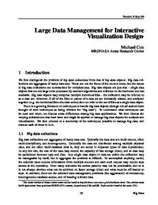
Figure 1: Streakline visualization of a 2 TB turbopump data set, with particles colored by pressure. Because the geometry is proprietary, the pump blades are not shown and some remaining geometry is decimated.
A BSTRACT This paper describes the methods used to produce an interactive visualization of a 2 TB computational fluid dynamics (CFD) data set using particle tracing (streaklines). We use the method introduced by Bruckschen et al. [3] that precomputes a large number of particles, stores them on disk using a space-filling curve ordering that minimizes seeks, then retrieves and displays the particles according to the user’s command. We describe how the particle computation can be performed using a PC cluster, how the algorithm can be adapted to work with a multi-block curvilinear mesh, how scalars can be extracted and used to color the particles, and how the out-ofcore visualization can be scaled to 293 billion particles while still achieving interactive performance on PC hardware. Compared to the earlier work, our data set size and total number of particles are an order of magnitude larger. We also describe a new compression technique that losslessly reduces the amount of particle storage by 41% and speeds the particle retrieval by about 20%. CR Categories: I.3.8 [Computer Graphics]: Applications; E.4 [Coding and Information Theory]: Data compaction and compression; D.1.3 [Programming Techniques]: Concurrent Programming—Parallel programming ∗ e-mail:
[email protected] [email protected] ‡ e-mail:
[email protected] † e-mail:
IEEE Visualization 2004 October 10-15, Austin, Texas, USA 0-7803-8788-0/04/$20.00 ©2004 IEEE
Keywords: visualization, particle tracing, large data, out-of-core, PC hardware, clusters, computational fluid dynamics. 1
I NTRODUCTION
Interactive visualization of data sets containing a terabyte or more is difficult to do even on the largest systems. Very few systems have enough memory to hold the data in memory. Out-of-core visualization using traditional visualization algorithms is impossible since the data rates of tens of gigabytes per second necessary cannot currently be achieved. However, it is currently quite possible to generate multi-terabyte data sets of CFD or physics calculations on today’s supercomputers. In addition, using PC-class hardware for the visualization is desirable since this allows scientists to examine their results on their desktop. One approach that scales to large data sets is to precompute the visualization. In most cases, the resulting geometry can be displayed interactively. For time-varying data, a visualization can be computed for each time step, and, if not too large, it can be animated. Otherwise, each frame can be rendered beforehand and shown as a static movie. However, all of these methods suffer from a lack of interactivity since the visualization computation must be repeated whenever the visualization parameters (particle seedpoint, isosurface value, etc.) are changed. The approach introduced by Bruckschen et al. [3] for interactive particle visualization does not have this limitation. By computing a large number of streaklines from a regular grid of seedpoints and storing them on disk, a subset of the traces can be retrieved and viewed interactively. This approach stores the traces on disk in a format that allows the streaklines to be read from disk quickly. Each
353
trace is stored contiguously. In addition, the traces are written to disk in the order of a Morton space-filling curve [13], also known as a Peano or z-curve. This ordering reduces the number of disk seeks required to retrieve a 3D box of seedpoints. In this paper, we describe several extensions to this work and the results of applying the resulting system to a 2 TB CFD simulation of a turbopump (see Figure 1). We extend the approach to allow for particle advection through a data set defined on a multiblock curvilinear grid, and to extract and save a set of scalar values for each particle that can be used to color the particles when later viewed. We also describe how the particle advection can be computed on a Beowulf cluster with a limited amount of memory per node and how the particle data can be reduced to about 60% of its original size. Finally, we describe a viewer implementation that interactively retrieves particles from a file server. The viewer uses a server process that runs on one or more file servers, retrieves particle data, and sends it to a display process running on a workstation. The viewer prefetches data from one or more file servers for increased performance. Overall, this new system completely changes how scientists can view particles in terascale data sets. Our previous system required hours to compute an animation of a streakline for a new set of seedpoints. The new system can show a new set of seedpoints in a fraction of a second. 2
R ELATED W ORK
Visualization of large data sets has been an area of active research. A commonly used technique is to precompute the visualization by saving a series of images or sets of geometry. Two of the many systems that use precomputation are IBM Visualization Data Explorer (now OpenDX) [1] and UFAT [11]. Out-of-core visualization is another approach to handling large data sets. Chiang et al. [5] propose a fast out-of-core technique for extracting isosurfaces using a precomputed disk-resident index; Chiang [4] has recently extended the technique to handle time-varying data. A different out-of-core technique is to load only the portion of the data needed to produce the visualization via demand paging [6]. While this technique supports particle tracing and other visualizations, it does not allow interactive visualization of terascale data sets. Ueng et al. [14] have implemented a different out-of-core particle tracing system that works with unstructured meshes. A different large data visualization technique is to stream the data through a series of filters that produce the visualization, as proposed by Ahrens et al. [2]. This technique scales to handle very large data sets, and can be run in parallel. It should allow interactive visualization if the data are not too large and the visualization is computed on a sufficiently large system. However, streaming systems are not suitable for particle tracing because streaming requires a priori knowledge of the data access pattern, which is not available with particle tracing. Finally, Heerman [10] documents many of the issues encountered when dealing with terascale data on a day-to-day basis. 3
A LGORITHM OVERVIEW
Our visualization approach has two phases that run at different times. The particle computation application runs as a preprocessing step, and the viewer application is used for the interactive visualization. The computation application uses the input data set and writes metadata, particle traces, and scalar values to disk. The viewer application shows the particles to the user. The particle positions are stored in a series of files, one per time step. Each file has the streaklines computed for each seedpoint stored contiguously, which allows the streakline to be read with one disk read. Furthermore, the particle traces are placed in the
354
0 1 8 9 2 3 10 11 16 17 24 25 18 19 26 27 top plane
4 5 12 13 6 7 14 15 20 21 28 29 22 23 30 31 second plane
32 33 40 41 34 35 42 43 48 49 56 57 50 51 58 59 third plane
36 37 44 45 38 39 46 47 52 53 60 61 54 55 62 63 bottom plane
0 1 8 2 3 9 12 13 16 top plane 4 5 10 6 7 11 14 15 17 bottom plane
Figure 2: 4×4×4 (left) and 3×3×2 (right) Morton curves.
file according to their Morton order [13], which means that traces for seedpoints near each other in physical space are usually near each other in the particle file, further reducing the number of disk seeks. Scalar values are stored separately, with a separate file for each scalar and time step combination. If the scalars were not stored separately, i.e., stored next to the particles in the file, during retrieval any unwanted scalar values would either need to be skipped using additional costly seeks, or read and discarded. The Morton order is based on a space-filling curve, and is the same as the ordering seen when performing a depth-first traversal of an octree’s leaf nodes. Figure 2 shows the Morton order of a 4×4×4 cube. Because the Morton order is only defined for cubes with powers-of-two sizes, we use a modified Morton order that handles arbitrary dimensions (one different than described in the literature). This order is the same one that you would get if you traversed a cube that was the smallest power of two possible enclosing the desired array, but did not count elements outside the array. Figure 2 has an example. The earlier implementation [3] has more details on how the Morton order reduces disk seeks. Each file has a header giving the length of each trace, followed by the particle traces. Unlike Bruckschen et al.’s implementation, which uses a single trace length for each file, our implementation stores variably-sized traces, which only contain particles remaining in the domain. While using a single trace length simplifies the data access and makes saving the particle trace lengths unnecessary, it would have increased the amount of uncompressed particle data by about 33% or 580 GB. We could have limited the excess storage by limiting the maximum trace length, but doing so would limit our ability to determine the amount of recirculation and particle mixing, an important CFD visualization task. Compressing singlelength particle traces would reduce the amount of extra storage, but we have not investigated this. We follow Bruckschen et al. by compressing the particles’ 32-bit floating point coordinates to 16 bits. The 16-bit values are computed by subtracting one corner of the mesh’s bounding box, dividing by the size of the bounding box, and quantizing the resulting fractions to 16 bits. This quantization cuts the storage in half, and will not change the visualization in most cases. Given the resolution of current screens, the quantized particle coordinates should place the particles on the screen with a position error smaller than a pixel unless the view only shows a very small fraction of the overall data set. Files containing scalar values simply have a series of lists, with the lists containing the corresponding scalar values for the particle traces. The scalar values are also quantized to 16 bits, again to reduce the amount of storage required. This quantization maps a given range of floating point values to the range of 16 bit values. Our current process finds this range by computing, in a preprocessing step, each scalar’s minimum, maximum, average, and standard deviation across the entire data set. The user can then use these val-
ues to select which range should be saved in the scalar values. In general, this process may require user intervention to pick the scalar ranges because the scalars may have outliers that are far beyond the range of nearly all the scalars. Including the outliers in the range of allowable scalars can cause a too-small number of unique values to be saved for the majority of saved scalars, degrading the resulting visualization. However, the data set used for this paper did not have outliers, so we used the minimum and maximum scalar values to specify the range of values to be saved. Since we do not limit the length of particle traces, the worst-case total number of particles over all the time steps is proportional to the square of the number of time steps. For this data set, the overall number of particles generated was not very far from the worst case: it is only 25% less than the worst-case number of particles. This results in large particle files and very long computation times (see Section 5). The average number of particles per particle trace will vary because it depends on data set properties, such as the magnitude of the velocity vectors or the size of the domain in the direction of the fluid flow. 4
C URVILINEAR DATA
Computing particles in a data set using a regular grid [3] is somewhat simpler compared to a curvilinear grid. Particle integration requires retrieving velocity values at arbitrary points in physical space. This is straightforward with regular grids, but is more complicated with multi-block curvilinear grids. These grids require point location code to find a cell enclosing the requested physical location, and additional code to resolve cases where multiple grids overlap. We use the Field Model library [12] for accessing velocity values, which simplifies the retrieval from an application’s point of view to a single function call once the grid has been read. An additional complication is that the domain of curvilinear grids are much more irregular than regular grids, which means that finding the seedpoints for the particle integration requires a bit more work. Like Bruckschen et al. [3], we use a regular grid of seedpoint locations. However, the regular grid of seedpoints is usually evenly spaced throughout the bounding box of the mesh (the user can specify a different box of seedpoints if an area is of particular interest). With many curvilinear grids, most of these initial seedpoints are outside the grid. In our data set, only 14% of the initial seedpoints are inside the grid. Figure 3 shows an example of seedpoints spread over the domain of a 2D curvilinear grid, and shows how the initial seedpoints can be either inside or outside the domain. We find the seedpoints inside the grid, the active seedpoints, at the start of the computation by testing whether each initial seedpoint is inside the grid domain. Our grid varies over time, which means that holes in the grid that correspond to the interior of a turbine blade can move over time. Thus, we test each initial seedpoint against a number of different grid time steps; seedpoints inside any time step are considered active seedpoints. We test twenty time steps each spaced three time steps apart (i.e. time steps 0, 3, 6, ..., 57). We need to test 60 time steps since that is the amount of time needed for a blade to advance one blade width, which lets any initial seedpoint inside a blade at the first time step find that it is inside the grid domain. Testing every third time step speeds this initial checking. The number and spacing of time steps to check is configurable since it is data set dependent. Once the validity of each initial seedpoint has been determined, the computation algorithm writes out a metadata file. This file has the dimensions of the initial seedpoint grid, the box containing the initial seedpoints, the grid bounding box, the number of active seedpoints, and a value for each initial seedpoint. This value is –1 if the seedpoint is not active, and is the number of the active seedpoint otherwise. This array of values is needed because the particle files only contain traces for the active seedpoints; otherwise the viewer
Figure 3: Example of 2D curvilinear mesh with two grid blocks, shown in black and blue. Seedpoints are spaced evenly throughout the grid’s bounding box. Seedpoints inside the domain are colored green, and those outside are red.
application would not be able to determine which selected initial seedpoints have particle data, nor the position of the valid seedpoints within the particle files. Another option with curvilinear grids is to place seedpoints evenly in computational space. Computational space seeding is clearly desirable when the scientist would like to see particles placed around a moving object, such as a rotating turbine blade. Computational seeding might be considered superior because the seedpoint density follows the cell density, although the density of particles in cells will not be constant once the particles have been advected a significant distance. Our experience with the current system indicates that computational space seeding is not necessary for the particle visualizations needed for this data set. 5
PARTICLE C OMPUTATION
The particle computation was done on a 49-node Beowulf cluster (see Section 8). Dividing up the particle computation among the nodes was straightforward since the calculations for each seedpoint are independent. However, getting the data to the calculation was difficult since we obviously cannot load the entire 2 TB data set into each node’s 1 GB of memory, or even onto each node’s 100 GB disk. The amount of data needed at once can be greatly reduced by only loading pairs of time steps (both grid and solution) at a time, advancing the particles, and then loading the next time step [11]. However, this would still require 1.7 GB of memory, and would cause a lot of page swapping and low CPU utilization. We use several techniques to reduce the data and memory requirements, as described below. We use the following system architecture. The input CFD data are stored on a file server with 4.5 TB of disk. Each node reads the input data it needs from the file server, and sends the computed particles and scalars to the master node. The master node buffers the computed particles , and writes them to each output file in order. The output files are stored on the file server using NFS. The seedpoints are divided into 196 equal-sized chunks (4 chunks per node). Each chunk of particles is a contiguous section of the active seedpoints, sorted by Morton order. Using sections of contiguous seedpoints means that the particles do not fill the entire domain. This reduces the amount of solution data that must be loaded via demand paging, described below. Seedpoints in different areas of the domain will need different amounts of computation. For example, seedpoints near the domain exit will have shorter traces than ones near the domain entrance. We give each node 4 disparate chunks of seedpoints to reduce load imbalances caused by this effect. We reduce the memory usage via several techniques:
355
• Loading only a pair of time steps at a time, as described above. • Reducing the particle memory footprint. This is significant since each node will have about 4 million particles at the end of the computation. Our initial particle tracing code was very general (allowing particles constrained to a computational plane, streaklines or streamlines, etc.) and stored several intermediate results for increased speed, and used over 200 bytes per particle. We reduced the memory to 24 bytes per particle by removing unnecessary features and not storing the intermediate results. • Exploiting the regularities in the grid, as described below. • Using an out-of-core algorithm to load solution data via demand paging, also described below. 5.1
Exploiting Mesh Regularities
The mesh has 35 blocks, or zones, each representing a part of the domain. Many of the zones contain vertices near various features, such as turbine blades. Some of the zones rotate over time, such as those surrounding the rotating blades of the turbine (see Figure 1; the white gaps show the blade positions). Other zones do not change over time. Furthermore, many of the zones are rotated copies of other zones in the same time step, such as the zones that contain points around each of the blades. We used the techniques described in [9] to find the regularities described above and replaced the time-varying mesh (contained in 2400 mesh files) with a replacement mesh that required that only 46% of one mesh file be loaded. The replacement mesh uses three zones that refer to static data, four zones that rotate over time, 15 zones that rotate over time and can reuse the vertices from another zone, and 12 zones that are static and can use rotated vertices from another zone. All of the zones have unique per-vertex flags which indicate validity and correspondences between zones. Since the per-vertex flags in the turbopump data set do not vary over time, only all of the per-vertex flags from a single time step must be loaded. Using the replacement mesh cuts down the amount of mesh data by over a factor of 5000. (However, not all of the original mesh data would need to be loaded if the demand paging techniques described below are used.) The ability to exploit mesh regularities varies according to the data set. However, we believe such regularities are fairly common in data sets with time-varying meshes, although time-varying meshes are not that common. We have seen regularities in a simulation where the aircraft body rotates, and expect that such regularities would exist in a simulation of an aircraft with rotating propellers. 5.2
Demand-Paging Solution Data
Because each cluster node computes particles for seedpoints clustered in a few parts of the domain, each node does not access all of the solution data (the velocity values). We avoid loading unnecessary solution data by using demand paging, which is similar to the virtual-memory system used in most operating systems. This technique divides each solution file into a number of fixed-size blocks. When a solution file is opened, a data structure is created that indicates whether a given block is present, and points to the block if it is. Then, when solution data are requested, the data retrieval code checks whether the corresponding blocks are present, loads the blocks if not present, and then retrieves the requested data from the blocks. The data blocks are allocated from a fixed-size pool of blocks. If a block is needed when all the blocks are allocated, an in-use block that has not been recently accessed is chosen and reused. Each block contains an 8×8×8 cube of solution values,
356
Size of grid files Size of solution files Number of time steps Total data set size
381 MB 476 MB 2400 2055 GB
Initial seedpoint grid size Number of initial seedpoints Number of active seedpoints Total number of particles Particle storage (uncompressed) Particle storage (compressed)
35×167×167 976,115 135,443 293 billion 1761 GB 1021 GB
Table 1: Initial data set and particle data statistics (M=10 6 , G=109 ).
which reduces the number of blocks needed compared to blocks of data organized in standard array order. More details about this technique can be found in [6]. Unfortunately, the computation must wait while a block is loaded from the file server. We reduce this waiting by using a number of different threads, each working on a trace from a different seedpoint. When a thread starts waiting for a block of data, a different thread is made runnable (if one is available) so the processor is kept busy. This multithreading technique is also used to provide work for the two processors in each node. We speed the retrieval of blocks from the file server by using a custom protocol that allows multiple outstanding read requests, and only sends the requested data. Using this protocol increases the speed compared to using NFS. See [8] for more details about the multithreading technique, the remote protocol, and their associated speedups. The particle computation algorithm reduces the latency due to loading solution data by prefetching blocks when a new time step is started. If the previous time step calculation used files t and t + 1, the new time step calculation will use files t + 1 and t + 2. When the new step is started, a separate thread finds which blocks are currently present for file t +1 and quickly loads them for file t +2. This prefetching is effective because there is a high correlation between the particle positions, and hence the blocks used, in adjacent time steps. However, our unsophisticated prefetching scheme will load all the blocks that were either used in or prefetched for one time step even if they are not used in future time steps. To reduce the amount of unused prefetched data, no prefetching is used for every tenth time step. The spacing of 10 time steps was chosen arbitrarily. 5.3
Particle Computation Performance
The particle computation is fairly slow: the computation for the 2 TB data set took five days on the cluster described in Section 8. Table 1 shows some statistics about the run. While five days is a long time, it is much shorter than the weeks required for the original simulation, which was done on a larger machine. The computation saved particle locations as well as each particle’s age, pressure, x component of the velocity field, and velocity magnitude. The x component of the velocity field can be used to find reverse flow in the pump. The main performance limitation of the precalculation is loading the solution data from the file server. The CPU utilization on each node is quite low at the start of the computation for each time step since the CPU is waiting for data. Once enough data have been loaded, the CPU utilization rises to near 100%. Prefetching data for the next time step during the current time step would reduce this waiting period, and it would be best if the prefetching was done when no other requests for data were outstanding. However, this would require another time step of solution data to be loaded into memory, and it does not appear that the additional memory is available on our current cluster. A second performance limitation
Fraction of Original Size
1.5
1.0
Particles Velocity Magnitude
0.5
Pressure Particle Age 0.0
0
600
1200
1800
2400
zlib setting Default Filtered Huffman Only
No 97 97 97
Particles 0th 1st 66 57 67 57 72 59
2nd 98 99 99
No 79 79 79
zlib setting Default Filtered Huffman Only
No 57 59 69
Pressure 0th 1st 43 44 42 43 46 45
2nd 70 72 77
Velocity Magnitude No 0th 1st 2nd 84 61 59 90 85 61 58 91 86 66 59 91
Particle Age 0th 1st 4.3 5.2 4.3 5.2 15 16
2nd 81 81 81
Table 2: Size of particle and scalar files as a percentage of the original data size using the default zlib effort setting. Key to columns: No = no prediction, 0th = zeroth order prediction, 1st = first order, 2nd = second order.
Time Step
Figure 4: Compressed file size for particles and three scalars expressed as a fraction of the original file size, for each time step. The first two or three compressed files for scalars are larger than 1.5 times the original file size, and are omitted for clarity. See text for compression settings. The fluctuations in the pressure file sizes are caused by pressure waves in the data set.
is the fact that our load balancing is done statically, when the run starts, by dividing the seedpoints equally between the nodes. Since seedpoints have traces of varying length, this will cause load imbalances. We have found that the threading library greatly affects the performance. An earlier particle computation when our cluster was running a Linux 2.4 kernel took nearly three times as long as the current run that used a Linux 2.6 kernel. We believe the improved threading implementation in the 2.6 kernel caused the performance improvement since our code was not changed significantly. More evidence that the threading implementation affects the performance comes from our earlier work [8]. The experiments done for that paper, done on an SGI system running Irix, showed that the performance using the native sproc() thread library gave much better performance than the then-new pthreads thread library. 6
C OMPRESSION
Since the computed particles use a large amount of disk space, even after the 16 bit quantization, we have explored compressing the particle files. We used a prediction preprocessing step that reduced the entropy of the data as well as the zlib compression library [7], used by gzip. The prediction step uses particles earlier in each trace to compute the predicted value, and the difference between the actual and predicted value is compressed. Using previous values in a sequence to predict future values is a standard compression technique. We tried several different prediction methods as well as different zlib compression settings. All of the compression methods are lossless. The prediction methods tried were no prediction, and zeroth, first, and second order prediction. Zeroth order prediction predicts each particle or scalar value to be the same as the previous particle. First order prediction uses the formula pi = xi − 2xi−1 + xi−2 , where pi and xi are the i th preprocessed and original particle or scalar in the trace, respectively. First order prediction predicts that the particles travel in a straight line. Second order prediction uses the formula pi = xi − 3xi−1 + 3xi−2 + xi−3 . The compression results are shown in Table 2, which has the results if every tenth time step is compressed. The table does not show the results when the maximum zlib effort setting was used because
it had only negligible effect in nearly all the cases, and in many cases significantly increased the compression time. Using maximum effort when compressing the particle age values did slightly decrease the amount of storage needed from 4.3% to 3.9% of the original size, but took three times as much CPU time. By comparing different rows in Table 2, you can see that the other zlib setting, the compression method, had a significant effect on the amount of compression in only a few cases. The default setting and the filtered setting (the latter modifies the algorithm to work best with preprocessed input data) have nearly the same compression performance. Using Huffman-only compression gave about the same compression performance. However, Huffman-only compression took about half the time to compress the data, and sped the viewer retrieval process by about 10% since it is a much simpler algorithm. Comparing different columns in the table reveals that the prediction method had the most influence on the amount of compression. Not using any prediction did not get much compression of the particles, and allowed some compression of the scalar values. Using zeroth or first order prediction gave about the same amount of compression, and gave the best results. Second order prediction performed the worst. An explanation for this is that the second order prediction’s assumption that the first derivative is constant is false. The compression ratios for the particles and different scalar values were quite different. The ratios for particles and velocity magnitude values were about the same. Particle ages compressed very well; the best results had over 20 to 1 compression. This is not surprising since the ages for particles in a given trace, if all particles are still active, is a sequence of ages amax , amax − 1, ...1, 0, where amax is the maximum particle age. Particles that have been deleted cause gaps in the sequence. Comparing the ratios for pressure and velocity magnitude show that the compression is data-dependent. We have chosen to use two compression settings. When compressing particles, pressure values, and velocity magnitude values, our implementation uses first-order prediction, Huffman-only compression and the default effort setting. This results in slightly larger files, 59% of the original size instead of 57%, but increases the viewer performance. We use a different setting when compressing particle ages: zeroth-order prediction, standard compression algorithm, and the default effort setting. This gives an excellent level of compression without long compression times. These compression times were used in Figure 4 to show how the compression ratio varies over the time steps. The initial time steps did not compress at all because the compression algorithm does not work well on very short sequences, and because the increased bookkeeping data used in compressed files is noticeable with very short traces. The amount of storage reduction decreases quickly once the traces have about 100 particles. The compression ratio then slowly
357
• Time modified and selection box held constant. The viewer requests the particle traces for each requested time step and displays them.
drops to about 30% as the trace length increases. A possible explanation for the smaller compression ratio is that more fully evolved traces are much more complex than short traces, which results in less compression. The particle file format is slightly different with compressed particle traces. Instead of storing the number of particles in each trace in each file’s header, we store the compressed size of each particle trace, which requires a 32-bit integer. The 16-bit particle count is moved to the beginning of each trace. Including the count allows the compression algorithm to store uncompressed traces if the traces cannot be compressed, and also simplifies allocating memory for the uncompressed traces. Files with scalar values also have a header indicating the compressed size of each list of scalars. These files do not have the particle counts since they are already stored in the particle trace files. Compressing the particle traces and scalars is currently done as a post-process to the particle computation, and takes about a day due to limited disk bandwidth. If the compression was done during the particle computation, it would add only about 90 minutes of time to the run since the particles would already be in memory. 7
V IEWER
Once the particle traces have been computed, a separate application allows the traces to be viewed interactively. The viewer application has two components, which are separate programs: a workstation component, which runs on a workstation and handles user interaction and graphical display, and a server component, which runs on the file server and reads the requested traces from disk. The two components communicate using a custom protocol and a TCP connection. For increased performance during animation, multiple instances of the server component can be run on one or more file servers, providing interleaved access to time steps. The viewer allows interactive manipulation of the viewpoint and the selected seedpoints. It also allows interactive manipulation of the current time step or allows time to move forward automatically, animating the particles. Seedpoint selection is done using a selection box widget, which allows arbitrary axis-aligned selections. The widget allows changing the size or position of the selection via a direct manipulation interface. An additional viewer feature is that the viewer allows other precomputed geometry, such as surfaces or cutting planes, to be displayed with the particle traces. The geometry can be static, time-varying, or rotating at a constant rate. The additional geometry allows the particles to be visualized in the context of the overall data set. Finally, the viewer allows the particles to be colored according to one of the scalar values saved during the computation step. The viewer was written with attention to performance. When the particles are being animated, it overlaps the display with the retrieval of the next time step’s particles. Particle retrieval is optimized by reading multiple adjacent particle traces in a single I/O request. Unlike the implementation by Bruckschen et al., our implementation does not read particle traces that are not needed in the interest of reducing the number of disk seeks. We compared the performance of a viewer implementation that read unnecessary data to one that read only the necessary data, and did not see any speedup. Thus, we chose the simpler implementation, the one that reads only the needed data. The viewer operates differently depending on the interaction mode: • Time held constant and selection box modified. In this mode, the viewer requests any necessary particle traces and scalar lists from the server. Retrieved traces are saved in memory to avoid retrieving the same trace multiple times. The cache is flushed when the current time step is changed.
358
• Time animated and selection box held constant. When the particles are animating, the workstation component fetches the next time step’s particles while the current particles are being displayed. The server component sends the requested particles, and, if time is available, fetches particles for the next time step, which is two time steps ahead of the time step being displayed. • Time animated and selection box modified. This mode is similar to the previous mode except that the modified selection box causes the prefetching to not retrieve all of the necessary particles. The workstation component requests the missing particles via a second request. Unfortunately, this second request slightly decreases the response rate. This is partially alleviated by applying selection box changes to the next frame’s prefetch request. 8
E QUIPMENT
The particle computation was done on a 49 node Beowulf cluster. Each node had two 1.67 GHz Athlon MP processors and 1 GB of memory, and had a Fast Ethernet network connection. The master node was similar but had 2 GB of memory and Gigabit Ethernet. The input data as well as the computed particles were stored on a pair of file servers. Each had two 3 GHz Xeon processors, 4 GB of memory, dual channel-bonded Gigabit Ethernet, and 21 250 GB data disks. These IDE disks were organized into three hardware RAID 5 arrays that were then striped using software, resulting in 4.5 TB total storage per system. The viewer timings were done on a workstation that had two 3 GHz Xeon processors, 4 GB memory, Gigabit Ethernet, and a NVIDIA Quadro FX 3000 graphics card. All the systems ran Fedora Core 2 Linux. 9
P ERFORMANCE
We measured the speed of the viewer application for a few different configurations so we could gauge its overall speed, and quantify the effect of using compression, different numbers of servers, and displaying particles colored by scalar. All of the measurements used the turbopump data set and the same set of particles and seedpoints. Each run measured the time the viewer application took to retrieve a static selection of seedpoints for each of the time steps in the simulation. The performance figures are for runs that do not include any additional reference geometry in the viewer. We measured several different configurations, as shown in Table 3. One configuration used uncompressed particles; the others used compressed particles and different combinations of either one or two servers, and no scalars, particle age, and pressure. Each configuration was run using two different particle selections: a small selection near the middle of the pump and a larger one near the pump’s inlet. Table 3 gives some statistics about the selections and the resulting performance, and Figure 5 shows a few representative frames of the visualizations resulting from the two selection boxes. The small selection box contained a 5×7×8 array of seedpoints and had one row of missing seedpoints because the box was not entirely in the domain. The frame rate when using this selection, uncompressed particle traces, and one server was 5.1 frames per second. Using compressed traces increased the speed to 6.1 frames per second, an 18% speedup. Adding a second file server doubled the frame rate to 12.2 frames per second. When running with compressed particles, the viewer has the frame rate that is high enough
Statistic Number of seedpoints Average number of particles Maximum number of particles Average trace length Average Frame Rate Uncompressed particles Compressed particles Compressed particles Comp. particles with age Comp. particles with age Comp. particles with pressure Comp. particles with pressure
Small Selection 275 266,158 420,035 968 Servers 1 1 2 1 2 1 2
Large Selection 512 577,192 1,091,097 1,127
Small 5.1 6.1 12.2 3.5 6.5 2.4 4.5
Large 2.6 3.1 6.4 2.0 3.9 1.2 2.4
Table 3: Statistics (top) and viewer performance (bottom) for two selection sizes. The frame rates are given in frames per second.
to allow easy interaction. The frame rates when showing scalar values mapped onto the particles were significantly lower since data must be retrieved from two files instead of one. The large selection box contained an 8×8×8 array of seedpoints. This is the same number of seedpoints used in the measurements by Bruckschen et al. [3]. However, our visualization had a larger average trace length, 1,128 particles, than the maximum trace length of 130 particles used in the earlier paper. (Of course, comparisons between the two implementations and data sets are difficult due to equipment differences.) The frame rate with the larger selection box and uncompressed particle traces was 2.6 frames per second, which is a bit low. Using compressed traces on one server increased the frame rate by 23%, to 3.1 frames per second. Animating the particles using compressed traces and two file servers ran at 6.1 frames per second, nearly twice the speed. Overall, using particle trace compression results in a noticeable performance improvement in the viewer. In addition, using two servers instead of one adds a large performance boost since disk reads can be done in parallel. The above measurements only give performance information for one mode of operation: when the particles are being animated with a static selection box. Other modes have different performances. Changing the selection while animating has somewhat lower performance since the particle prefetching does not retrieve all of the needed particles. Interactively modifying the time step is also a bit slower since prefetching cannot be used. However, changing the selection box when time is held constant is quite fast. It is fast because many of the particle traces displayed with the previous selection box can be reused with the new selection box since the boxes almost always overlap. 10
C ONCLUSIONS AND F UTURE W ORK
In this paper, we have shown that the method of visualizing particle flow by precomputing particle traces for later retrieval and display can be scaled to handle multi-terabyte data sets and more than a terabyte of particles. We have discussed the necessary modifications to Bruckschen et al.’s original algorithm that allow a data set with a curvilinear mesh to be used, that allow the particle computation to be done using a PC cluster, and allow scalar values to be extracted and used to map color onto the particles. In addition, a new compression technique allows the particle traces to be compressed by 41%, saving a significant amount of storage space, and also improves the interactive viewer performance by roughly 20%. Overall, we have demonstrated a visualization system for a multiterabyte CFD data set that decreases the turnaround time for seeing
the results from changing the location of a streakline’s seedpoint location from hours to a fraction of a second. Future work includes improving the speed of the particle computation, either by improving the prefetching algorithm or by implementing dynamic load balancing. We would also like to improve the viewer by adding conditional display of particles based on their scalar value. For example, a conditional display of particle ages could allow the display of timelines, where particles are emitted every n time steps. 11
ACKNOWLEDGMENTS
We could like to thank Cetin Kiris for providing the data set utilized in our experiments, Tim Sandstrom for writing the program we modified to create the viewer application, and the anonymous reviewers for their comments. This work was funded by the NASA Computing, Information, and Communications Technology (CICT) Program, partially via NASA contract DTTS59-99-D00437/A61812D. R EFERENCES [1] Greg Abram and Lloyd Treinish. An extended data-flow architecture for a data analysis and visualization. In Proceedings of Visualization ’95, pages 263–270. IEEE Computer Society Press, 1995. [2] James Ahrens, Kristi Brislawn, Ken Martin, Berk Geveci, C. Charles Law, and Michael Papka. Large-scale data visualization using parallel data streaming. IEEE Computer Graphics & Applications, 21(4):34– 41, July/August 2001. [3] Ralph Bruckschen, Falko Kuester, Bernd Hamman, and Kenneth L. Joy. Real-time out-of-core visualization of particle traces. In Proceedings IEEE 2001 Symposium on Parallel and Large-Data Visualization and Graphics, pages 45–50. IEEE Computer Society Press, October 2001. [4] Yi-Jen Chiang. Out-of-core isosurface extraction of time-varying fields over irregular grids. In Proceedings of Visualization 2003, pages 217–224. IEEE Computer Society Press, October 2003. [5] Yi-Jen Chiang, Cl´audio T. Silva, and Willian J. Schroeder. Interactive out-of-core isosurface extraction. IEEE Visualization ’98, pages 167– 174, October 1998. [6] Michael B. Cox and David A. Ellsworth. Application-controlled demand paging for out-of-core visualization. In Roni Yagel and Hans Hagen, editors, Proceedings of IEEE Visualization ’97, pages 235– 244. IEEE Computer Society Press, October 1997. [7] P. Deutsch and J.-L. Gailly. RFC 1950 - ZLIB compressed data format specification version 3.3, 1996. [8] David Ellsworth. Accelerating demand paging for local and remote out-of-core visualization. Technical Report NAS-01-004, NAS Division, NASA Ames Research Center, June 2001. [9] David A. Ellsworth and Patrick J. Moran. Accelerating large data analysis by exploiting regularities. In Proceedings of Visualization 2003, pages 561–568. IEEE Computer Society Press, October 2003. [10] Phillip D. Heerman. Production visualization for the ASCI one teraFLOPS machine. In Proceedings of Visualization 1998, pages 459– 462. IEEE Computer Society Press, October 1999. [11] David Lane. UFAT: A particle tracer for time-dependent flow fields. In Proceedings of Visualization ’94, pages 257–264. IEEE Computer Society Press, October 1994. [12] Patrick Moran. Field model: An object-oriented data model for fields. Technical report, National Aeronautics and Space Administration, 2001. NAS-01-005. [13] Hans Sagan. Space-Filling Curves. Springer-Verlag, New York, 1994. [14] Shyh-Kuang Ueng, Christopher Sikorski, and Kwan-Lui Ma. Outof-core streamline visualization on large unstructured meshes. IEEE Transactions on Visualization and Computer Graphics, 3(4):370–380, December 1997.
359
Figure 5: Two particle trace visualizations of the turbopump data set. The left column images show a visualization using a small selection box in the middle of the domain, and the right column images show a larger selection box near the inlet. The images in the three rows show the visualizations at time steps 300, 1200, and 2100 (respectively, top to bottom). The particles in the images on the right are colored according to their age. Because the geometry is proprietary, the pump blades are not shown and some remaining geometry is decimated.
360