arXiv:1605.09497v1 [cs.GT] 31 May 2016
Interdependent Scheduling Games Andres Abeliuk Data61/NICTA
[email protected]
Haris Aziz Data61/NICTA and UNSW
[email protected]
Gerardo Berbeglia University of Melbourne
[email protected]
Serge Gaspers UNSW and Data61/NICTA
[email protected]
Petr Kalina Czech Technical University
[email protected]
Nicholas Mattei Data61/NICTA and UNSW
[email protected]
Dominik Peters University of Oxford
[email protected]
Paul Stursberg Technische Universit¨at M¨unchen
[email protected]
Pascal Van Hentenryck University of Michigan
[email protected]
Toby Walsh UNSW and Data61/NICTA
[email protected]
Abstract We propose a model of interdependent scheduling games in which each player controls a set of services that they schedule independently. A player is free to schedule his own services at any time; however, each of these services only begins to accrue reward for the player when all predecessor services, which may or may not be controlled by the same player, have been activated. This model, where players have interdependent services, is motivated by the problems faced in planning and coordinating large-scale infrastructures, e.g., restoring electricity and gas to residents after a natural disaster or providing medical care in a crisis when different agencies are responsible for the delivery of staff, equipment, and medicine. We undertake a game-theoretic analysis of this setting and in particular consider the issues of welfare maximization, computing best responses, Nash dynamics, and existence and computation of Nash equilibria.
1
Introduction
Restoring critical infrastructure in the aftermath of natural disasters or extreme weather events where water, power, and gas services may all be interrupted is one of the most important ways of limiting the impact of the disaster on society. Our motivation for this work is drawn from situations where companies and governments need to restore interdependent infrastructure after major disruptions due to disasters and other forces. For instance, the electric company may be able to restore power lines to individual homes, but no electricity will
flow until the gas company can supply gas to the main generator. Once the power is flowing, the electric company receives its reward (income) from those customers receiving power. In order to pump water, power needs to have been restored and the water lines need to be repaired. Each of these objectives are typically broken down into smaller tasks that restore availability to a subset of customers. In these settings, multiple agents (also called players) are responsible for different services and may have conflicting interests: the power company may deploy its services in an order that maximizes reach to its subscriber base first, as opposed to undertaking repairs that allow another company to restart the water pumps. This paper formalizes a novel abstract model of this setting and studies the problem of finding a joint deployment schedule of services through a game theoretic lens, as players in this setting are independent decision makers. We consider classic questions such as welfare maximization, best responses, and the existence and computation of Nash equilibria. From the community’s perspective, the overall goal is to reduce the size and length of the blackout. Indeed, governments in the US plan for infrastructure restoration at a higher level than the individual company, e.g., the state government or regional emergency management planning. However, when disasters become too large or individual companies refuse to cooperate with regional disaster management plans then companies might be unable (or unwilling) to obey global welfare considerations in restoring their infrastructure. Cavdaroglu et al. [2013] and Coffrin et al. [2012] provide models that integrate the restoration planning and scheduling decisions to show that there is significant value in this integration as opposed to tackling both problems in a decentralized manner. Our model of interdependent scheduling games (ISGs) is a step towards understanding the im-
pact of decentralized decision making in settings with interdependencies. Other examples of ISGs include coordinating multiple providers for humanitarian logistics over multiple regions, where roads need to be repaired before supplies can be delivered and tents must be erected before supplies can be distributed, or the coordination of interdependent supply chains which may involve ports, terminals, railway, and truck operators [Van Hentenryck et al., 2010; Simon et al., 2012]. In our formalization, we consider a set of players, each of which has a set of services under their control that need to be deployed. The individual players’ services may have dependencies among each other and, crucially, may also be dependent on the status of other players’ services. In contrast to most traditional scheduling settings, where a task cannot be scheduled unless all of its dependencies have been fulfilled, services in our setting can be deployed at any time, even before its dependencies have been deployed. However, a player only starts accruing reward for a service v once all of its dependencies have been deployed as well. At this point, we say that v has been activated and the player continues to gather reward for every time step in which the service is active. A typical reward in our setting would be collecting fees from utility subscribers who have had their service restored. Contributions. We present a scheduling model with dependencies among services that is suitable for scenarios in power restoration after natural disasters. We show that when there is only a single player, a welfare-maximizing schedule can be found in polynomial time. For more players, welfare maximization becomes NP-complete even with just two services per player. Regarding game-theoretic solution concepts, we prove that in general, pure Nash equilibria are not guaranteed to exist, and that it is NP-hard to decide their existence. On the positive side, we consider a restricted setting where all services have uniform (equal) reward and prove that a pure Nash equilibrium always exists and can be computed in polynomial time. Similarly, best responses can be computed efficiently but they need not converge to a Nash equilibrium, even if rewards are uniform. For the uniform rewards case, we also give bounds for the price of anarchy and the price of stability. Further, we provide an ILP formulation of the problem and demonstrate that, for generated data, we can find welfare maximizing schedules quickly.
2
Related Work
The problem of finding a schedule of tasks that maximizes the reward is an important question in scheduling, a classic area of computer science with many practical and important problems. Most classical scheduling problems focus on allocating scarce resources to multiple tasks in order to maximize an objective function or minimize total time [Brucker and Brucker, 2007; Lee et al., 1997]. In contrast to most of the scheduling literature, the dependencies (or precedence constraints) between the services in our model do not prevent the player from scheduling a service before its prerequisites are fulfilled. Instead, they keep the player from receiving reward from the service until the prerequisites are fulfilled. Encouraging distributed agents, each of which may be re-
sponsible for only a small piece of a larger task, to work together to solve complex problems has a rich history in artificial intelligence and multi-agent systems research. Scheduling distributed tasks in domains where agents are imbued with their own reward functions but are ultimately cooperative as they can jointly benefit from finding coordinated schedules, has been studied in a probabilistic setting by Zhang and Shah [2014]. Additionally, task oriented domains [Rosenschein and Zlotkin, 1994], which typically involve multiple agents working together cooperatively, are a popular framework for investigating mechanisms and properties of multiagent domains where agents either need to work together or negotiate over work to be accomplished. Zlotkin and Rosenschein [1993] formalize the notion of strategic behavior when agents negotiate in task oriented domains. They provide a characterization of the type of lies (e.g. hiding jobs) and reward functions that admit incentive compatible mechanisms for a number of classic domains, though none of these classic domains involve scheduling with dependencies. We focus our analysis on game-theoretic issues such as best response dynamics and Nash equilibria that are keenly applicable in settings such as ours where agents, trying to maximize independent utility, may or may not have explicit incentives to cooperate towards maximizing global welfare. Scheduling domains in which players compete for common processing resources were introduced by Agnetis et al. [2000; 2004] and Baker and Smith [2003]. The most traditional approach in multi-agent scheduling is to consider a single centralized authority optimizing the whole domain. There have been a number of recent works focused on decentralized scheduling mechanisms. Agnetis et al. [2007] consider auction and bargaining models, which are useful when several players have to negotiate for processing resources on the basis of their scheduling performance. Scheduling auctions typically divide the schedule horizon into time slots, and these time slots are auctioned among the players. The bargaining approach considers two players that have to negotiate over possible schedules. Abeliuk et al. [2015] consider a twoplayer bargaining mechanism for any setting where the reward of one player does not depend on the actions taken by the other. Their results hence apply to special instances of ISGs with two players. For additional literature on mechanism design for non-cooperative scheduling games see, e.g, Heydenreich et al. [2007], Christodoulou et al. [2004], and Angel et al. [2006]. Another related line of research is multi-agent projectscheduling. Here, each project is composed of a set of activities, with precedence relations between the activities, and each activity belongs to an agent. Each activity is associated with a minimum and a maximum processing time and agents have to choose a duration for all their activities. Compressing the duration of an activity generates a cost to the agent, and an agents’ payoff is a fixed proportion of the total project payment, which depends on the project completion time. A mechanism design approach for multi-agent projectscheduling by Confessore et al. [2007] proposes a decentralized mechanism using combinatorial auctions. Recently, Briand and Billaut [2011] took a first step in analyzing game theoretical properties such as the existence and computation
of Nash equilibria as well as studying the price of anarchy in this setting. However, their setting significantly differs from that considered in this paper in that activities of the same agent can be processed in parallel and that all agents receive some fraction of the reward of a common production process. In contrast, we focus on agents involved in independent projects with separate objective functions, only related by precedence constraints between each other.
3
Our Model
A directed graph G is a pair (V, E) of a finite set of vertices V and a set of directed edges E ⊆ V × V where (u, v) ∈ E means that there is a directed edge from u to v in G. We will always assume that G is acyclic, i.e., there is no set of edges {(v1 , v2 ), (v2 , v3 ), . . . , (vn , v1 )} ⊆ E. We say that G is transitive if (u, v), (v, w) ∈ E implies that (u, w) ∈ E. The transitive closure of a graph G = (V, E) is a graph G0 = (V, E 0 ) such that (u, v) ∈ E 0 if a directed path connects u and v in G. The in-neighborhood of a vertex v is the set of − vertices with edges to v and is denoted by NG (v) = {u ∈ V : (u, v) ∈ E}. An interdependent scheduling game (ISG) with k players is given by a tuple ((T1 , . . . , Tk ), G, r). Each player i needs to schedule a set of services Ti , where the Ti are pairwise disSk joint. We denote the set of all services by T = i=1 Ti . We assume without loss of generality that |T1 | = · · · = |Tk | = q. Within T there are dependencies: a service will not activate until it and all its prerequisites are deployed. We formalize this dependency relation as a transitive acyclic directed graph G = (T, E). If (u, v) ∈ E, then service v will generate a reward only after service u has been deployed.To be precise, at each time step t, each player deploys exactly one service. In particular, we assume that every service takes exactly one unit of time to deploy. A service which takes longer to deploy can be represented as a series of services depending on each other where only the final service generates a reward. For each service v ∈ T , there is a reward r(v) ≥ 0, representing payment received or subscribers served in each time period that the service is active. We will sometimes consider the more restrictive case of uniform rewards where for all v ∈ T, r(v) = 1. A solution for an ISG is a schedule of all services in T . As rewards are non-negative, players do not have an incentive to leave a gap between the deployment of two services. We can hence represent a schedule by a tuple π = (π1 , . . . , πk ), where each πi : Ti → {1, . . . , |Ti |} is a permutation of the services Ti of player i. This permutation uniquely determines the schedule for player i and the position of a service in the permutation denotes the time when it is deployed. A service v is active during a time step if itself and all − services in NG [v] are deployed at or before that time step. We denote by a(v) the time when v becomes active, i.e. − a(v) = max{π(w) : w ∈ {v} ∪ NG [v]}. At each time step, all active services v generate the reward r(v). Thus, for a schedule Pq π = P (π1 , . . . , πk ), the utility of player i is Ri (π) = utilitarian social t=1 v∈Ti ,t≥a(v) r(v). TheP k welfare (or just welfare) of a schedule π is i=1 Ri (π). We graphically represent an ISG in Example 1. Player i’s services Ti form the nodes shown in the ith row. The services
in a row, from left to right, represent player i’s schedule, while the label of a service indicates its reward. For ease of presentation, we omit arrows that are implied by transitivity of the dependency relation; the full dependency graph is the transitive closure of the depicted graph. This representation is not completely unambiguous as a service v is identified only by r(v) and the edges in NG (v). However, while indistinguishable (subsets of) tasks may exist, these can be interchanged within any particular outcome without effect. Example 1. Consider the following example. π1 :
10
1
1
π10 :
1
1
10
π2 :
1
100
100
π20 :
100
100
1
Both of the services with reward 100 belong to Player 2 but depend upon a service belonging to Player 1. For schedule π, R1 (π) = 3 · 10 + 2 · 1 + 1 = 33 as the service with reward 10 is active for three time steps and the other services are active for two and one time step, respectively. Similarly, R2 (π) = 3· 1+2·100+100 = 303. For π 0 , R1 (π 0 ) = 3·1+2·1+10 = 15 while R2 (π 0 ) = 3 · 100 + 2 · 100 + 1 = 501. Hence, Player 1 can sacrifice some individual reward to increase welfare.
4
Best Responses
If all other players’ actions are fixed, the resulting problem for an individual player is that of finding a best response. Let Ri (π−i , πi0 ) be the reward for player i for the schedule (π1 , . . . , πi−1 , πi0 , πi+1 , . . . , πk ). Problem: ISG B EST R ESPONSE. Instance: An ISG ((T1 , . . . , Tk ), G, r), a schedule π−i for all players {1, . . . , k} \ {i}, and an integer W . Question: Is there a πi0 such that Ri (π−i , πi0 ) ≥ W ? Assuming that players are individually rational they will favor schedules that maximize their own reward, i.e., their own subscriber base or service network. Hence an individual player will always favor a schedule such that every service v that he controls is deployed only after all other services under the player’s control that v depends on have been deployed. Formally, the following Lemma holds: Lemma 1. Let ((T1 , . . . , Tk ), G, r) be an ISG with general rewards and π−i a schedule for all players except player i. Let Gi = (Ti , Ei ) denote the subgraph of G induced by the vertices in Ti . Then, there exists a best response πi for player i such that πi (u) < πi (v) for all (u, v) ∈ Ei .
(1)
Proof. Let σ(πi ) := |{v ∈ Ti : ∃(u, v) ∈ Ei with πi (u) > πi (v)}| denote the number of services in Ti that depend on another service in Ti which is scheduled later. Let πi0 denote a best response of player i such that σ(πi0 ) is minimal among all best responses. We suppose for contradiction that the statement is false, therefore σ(πi0 ) ≥ 1. Choose (u, v) ∈ Ei with πi0 (u) > πi0 (v) in such a way that there is no u0 with (u0 , v) ∈ Ei and πi0 (u0 ) > πi0 (u). Consider the following
modified schedule πi∗ for player i: 0 0 0 0 πi (w) − 1 πi (w) ∈ [πi (v) + 1, πi (u)] ∗ 0 πi (w) := πi (u) w=v 0 πi (w) else.
1. η(b) ≤ πi∗ (a). In this case, we set ∗ ∗ ∗ ∗ πi (w) + 1 πi (w) ∈ [πi (a), πi (b) − 1] ∗∗ ∗ πi (w) := πi (a) w=b ∗ πi (w) else.
The following two properties hold: (i): The schedule πi∗ is also a best response. The only service that is scheduled to a later time in πi∗ (and hence could cause itself or services depending on it to generate a smaller reward) is v. However, v did not activate before time step πi0 (u) under π 0 and as πi∗ (v) = πi0 (u) the reward generated by v does not change. The same holds for all services that depend on v. (ii): σ(πi∗ ) < σ(πi0 ). First, note that v does not contribute towards σ anymore as πi∗ (v) > πi∗ (u) (the same holds for all other services that v depends upon by the maximality of u). Now, consider any service w that did not contribute to σ(πi0 ). As the ordering among all services except v remains the same, such a w can only contribute to σ(πi∗ ) if it depends on v and πi0 (v) < πi0 (w) < πi∗ (v) = πi0 (u). But then, it must also depend on u by transitivity and hence it contributed to σ(πi0 ) already. From (i) and (ii), we obtain a contradiction to minimality of σ(πi0 ), concluding the proof.
The reward generated by b increases by πi∗ (b) − πi∗ (a), at the same time the reward of at most πi∗ (b) − πi∗ (a) services decreases by 1. Hence, π ∗∗ is still optimal and satisfies condition (1). Furthermore, (πi )−1 (k) = (πi∗∗ )−1 (k), contradicting π ∗ ’s maximality. 2. πi∗ (a) < η(b) < πi∗ (b). We construct a new schedule π ˜i∗ ∗ with π ˜i (b) = η(b) as above. Then, proceed as in 3. 3. πi∗ (b) ≤ η(b). Construct a schedule πi∗∗ as follows: Set πi∗∗ (b) := πi∗∗ (a). Let a0 be the earliest successor of a. If πi∗ (a0 ) > πi∗ (b), set πi∗∗ (a) := πi∗ (b) and πi∗∗ (w) := πi∗ (w) for all other services. Otherwise, set πi∗∗ (a) := πi∗ (a0 ) and let a00 be the earliest successor of a0 . Proceed with a00 (and possibly its earliest successor) as above until an earliest successor a∗ satisfies πi∗ (a∗ ) > πi∗ (b). The resulting schedule π ∗∗ is still optimal and satisfies condition (1). Furthermore, (πi )−1 (k) = (πi∗∗ )−1 (k), contradicting π ∗ ’s maximality. In all three cases, we reach a contradiction which proves that our assumption was wrong and πi is indeed optimal.
Note that performing pairwise swaps in a player’s scheduled services is not sufficient in the context of the above proof as this may introduce new forward edges. The above lemma holds for general rewards. If rewards are uniform, we can use Lemma 1 to derive a polynomial-time algorithm for an individual player’s best response to all other players’ schedules. Theorem 1. For an ISG with uniform rewards, there exists a polynomial-time algorithm to compute a best response. Proof. Consider the subgraph Gi of G induced by the set Ti of services belonging to player i. For every service u, denote by η(u) the lower bound on its activation time imposed by π−i . Formally, η(u) := max{π(v) : v ∈ T \ Ti , (v, u) ∈ E}. Note that (u, w) ∈ Ei implies η(w) ≥ η(u) by transitivity of Ei . We give a greedy algorithm that solves the problem optimally. Starting from the first time step, the algorithm successively schedules a service which minimizes η among all services with no incoming edges in Gi . Such a service always exists, as G (and hence all subgraphs) is acyclic. The service with all its (outgoing) edges is then removed from Gi . To prove that the algorithm yields an optimal solution, let πi be the outcome of the algorithm. Suppose for contradiction that πi is not optimal. Let πi∗ be an optimal schedule satisfying condition (1) (which exists by Lemma 1) maximizing the first time slot for which any such schedule differs from πi . Formally, there exists k ∈ N such that (πi∗ )−1 (i) = (πi )−1 (i) for all i < k and there is no optimal schedule πi0 satisfying condition (1) with (πi0 )−1 (i) = (πi )−1 (i) for all i < k + 1. Let a := (πi∗ )−1 (k) and b := (πi )−1 (k). Consider the subgraph of Gi from which the first k − 1 entries of πi (and hence of πi∗ ) have been removed. First, observe that a cannot have any incoming edges as πi∗ satisfies condition (1). Hence, it holds that η(b) ≤ η(a), otherwise the algorithm would have selected a rather than b. We distinguish three cases:
In contrast, we can obtain the following statement about general rewards by reduction from single-player welfare maximization using Theorem 5. Corollary 1. For an ISG with general rewards, computing a best response is NP-complete.
5
Welfare Maximization
A central planner would want to find a schedule that maximizes the welfare, i.e., the most profitable services in T activated for the longest amount of time. Problem: ISG W ELFARE. Instance: An ISG ((T1 , . . . , Tk ), G, r) and an integer w. Pk Question: Is there a π such that i=1 Ri (π) ≥ w? Intuitively, it might seem desirable to design schedules where no service has to wait for its activation after it has been deployed. We call such schedule conflict-free. For uniform rewards, if a conflict-free schedule exists then every welfare-maximizing schedule obviously has to be conflictfree. A similar statement holds for single-player games by the construction of πi∗ in Lemma 1 (proof omitted). Theorem 2. For one player and general rewards, every welfare-maximizing schedule is a conflict-free schedule. However, this property does not hold in the case of more than one player and general rewards. This can be seen by considering Example 1 and making all other services dependent on π1 ’s service with reward 10. Then, any conflict-free schedule will yield welfare 319 while the welfare-maximizing schedule is 417, yielding the following theorem: Theorem 3. For multiple players and general rewards, even if a conflict-free schedule exists, the welfare-maximizing schedule(s) might not be conflict-free.
Turning to computational complexity, we observe that for one player welfare maximization is equivalent to finding a best response, hence with Theorem 1 we get the following. Corollary 2. For uniform rewards, ISG W ELFARE can be solved in polynomial time for a single player. However, when we either increase the number of players (Thm. 4) or relax the restriction of uniform rewards (Thm. 5), the problem is NP-hard for surprisingly restricted cases. Theorem 4. ISG W ELFARE is NP-complete, even when the rewards are uniform and each player has two services. Proof. The problem is in NP since we can efficiently compute the welfare of a given schedule. For NP-hardness, we reduce from M IN 2SAT [Kohli et al., 1994] which asks: Given a 2CNF formula F where each clause contains exactly two literals, and an integer k, is there an assignment to the variables of F such that at most k clauses are satisfied? For each variable x in F , create a player Px with services Tx = {x, ¬x}. For each clause c in F , create a player Pc with services Tc = {c1 , c2 }. For each clause c = (`1 ∨ `2 ), the precedence graph contains (c1 , c2 ), (`1 , c1 ), and (`2 , c1 ). Rewards are uniform, and we set w = 3n + 3m − k, where n and m are the number of variables and clauses of F . It remains to prove that F has an assignment satisfying at most k clauses if and only if the ISG has a schedule generating a reward of at least w. For the forward direction, suppose F has an assignment α : var(F ) → {0, 1} satisfying at most k clauses. Consider the schedule where, for each variable x, the player Px schedules first the literal of x that is set to false by α, i.e., x is scheduled before ¬x iff α(x) = 0. Additionally, for each clause c, the service c1 is scheduled before c2 . This schedule generates a reward of 3 for each variable: a reward of 1 at the first time step and a reward of 2 at the second time step. For a satisfied clause c, the schedule generates a reward of 2: at the first time step no reward is generated since the literal satisfying the clause is scheduled at the second time step and there is an arc from that literal to c1 , and a reward of 2 is generated at the second time step. For an unsatisfied clause c, the schedule generates a reward of 3: since neither literal satisfies the clause, both literals are scheduled at the first time step. Thus, the utility generated for this schedule is at least 3n + 3m − k. For the reverse direction, let π be a schedule generating a reward of at least w. Consider the assignment α : var(F ) → {0, 1} with α(x) = 0 iff player Px schedules x at the first time step. Note that at the second time step, each player generates a reward of 2. Also, each player corresponding to a variable generates an additional reward of 1 at the first time step since his services have in-degree 0. So, at least 3n + 3m − k − (3n + 2m) = m − k additional clause players generate a reward of 1 at the first time step. But, for each such clause c, c1 is scheduled before c2 and both literals occurring in c are scheduled at the first time step, which means that the assignment α sets these literals to false. Therefore, α does not satisfy c. We conclude that α satisfies at most k clauses. Theorem 5. For general rewards, ISG W ELFARE is NPcomplete even for a single player.
Figure 1: Mean runtime of the ILP over 1,000 random ISG instances varying the number of players, services, and reward type; error bars represent one standard deviation (σ). The solid lines are instances with general rewards, the dashed lines are instances with uniform rewards. The plot is semilogarithmic, so a straight line represents an exponential increase in time. For the general rewards case, error bars are not included for clarity; for |Ti | ∈ {10, 30, 50} the numbers are small, σ = 30 seconds in the worst case, however, for 70 services and 10 players this balloons to 200 seconds. The proof, omitted for space, is a reduction from the NP-hard problem S INGLE MACHINE WEIGHTED COMPLETION TIME [Lenstra and Rinnooy Kan, 1978]. It relies on Theorem 2 and an adjustment of rewards.
5.1
Integer Programming Formulation
While the general problem of finding a welfare maximizing schedule for an ISG instance is computationally hard, it may still be solvable for instances of moderate size. The ISG W ELFARE problem admits a natural integer linear programming (ILP) formulation. For each service v ∈ T and time step t ∈ [q], we introduce two binary decision variables av,t and sv,t . Let sv,t = 1 if and only if service v is scheduled at time t, and av,t = 1 if and only if service v is active at time t. P Pq max v∈T t=1 av,t · r(v) P q s.t. ∀v ∈ T P t=1 sv,t = 1 s = 1 ∀i ∈ [k], ∀t ∈ [q] v,t v∈T Pit ∀v ∈ T, ∀t ∈ [q] av,t ≤ t0 =1 sv,t0 av,t ≤ aw,t ∀(w, v) ∈ E, ∀t ∈ [q] We implemented the ILP and solved 1000 randomly generated instances where (a) general rewards are drawn from [50,100] and (b) rewards are uniform. The dependency graphs are generated by first randomly permuting the list of all services; then for each service i, drawing a random number of child services c ∈ {0, 1, 2} and adding edge (i, i + c) with probability 0.5. Increasing the number/likelihood of dependencies by increasing the potential number of children or increasing the connection probability significantly increases
runtime. Figure 1 shows the results for different parameters using Gurobi 6.5 on a computer equipped with an 2.0 GHz Intel Xeon E5405 CPU with 4 GB of RAM. The results suggest that, despite worst case hardness, the running times remain feasible, at worst ≈ 600s, for practically relevant problem sizes: up to 10 players with 70 services each.
6
Nash Dynamics and Equilibria
We now turn to the situation where players may respond to each other’s schedule changes. This is an important question for game theoretic analyses as it allows us to see which states leave no incentives for self-interested players to deviate; and what can happen when players are continually responding to the moves of one another. An important first question is whether a sequence of best responses terminates. Theorem 6. For ISGs with uniform rewards, best responses can cycle. Proof. Consider the following example depicting a sequence of best responses. Starting with the lower right schedule πD we move to the upper left schedule πA where Player 2 has changed his schedule in a best response to πD . We then read left to right, top to bottom, to end up back at πD . π1A :
c
a
d
b
π1B :
d
b
c
a
π2A :
d
a
c
b
π2B :
d
a
c
b
π2A response to π1D R(π1A ) = 8, R(π2A ) =
π1B R(π1B )
10
response to π2A = 10, R(π2B ) =
π1C :
d
b
c
a
π1D :
c
a
d
b
π2C :
c
d
b
a
π2D :
c
d
b
a
π2C response to π1B R(π1C ) = 9, R(π2C ) = 10
6.1
8
π1D response to π2C R(π1D ) = 10, R(π2D ) = 9
ISGs with Uniform Rewards
A schedule π is in pure Nash equilibrium (PNE) if no player can obtain strictly more utility by unilaterally changing his own schedule; formally, Ri (π−i , π) ≥ Ri (π−i , πi0 ) for all players i and all schedules πi0 of player i. For instance, note that the above example, despite having a sequence of best responses that cycle, does admit the PNE depicted below:
− Let Ni− (v) := (NG (v) ∪ {v}) ∩ Ti denote the closed in(t) neighborhood of service v under player i’s control, Ti the set of services of player i already scheduled before iteration t (t) (t) and αi := |Ti |. In every iteration, we will choose a service and schedule it together with all remaining services that it (t) depends on. This means that for a service v ∈ Ti , a(v) is well-defined during iteration t. We can therefore define ( (t) maxw∈N − (v) a(w), Ni− (v) \ Ti = ∅ (t) i η¯i (v) := (t) (t) αi + |Ni− (v) \ Ti |, else (t)
Now, η¯(t) (v) := maxi∈N η¯i (v) represents a tight lower bound for a(v) in any schedule which is a “completion” of the partial schedule from iteration t (achieved if v and all prerequisites are scheduled immediately). Similar to Theorem 1, it can be verified that player i’s schedule πi is a best response if for every iteration t and player i, the condition (1) from Lemma 1 holds for all ser(t) (t) (t−1) vices v, w ∈ Ti and if v ∈ Ti \ Ti , then η¯(t−1) (v) (t−1) is minimal among all services from the set Ti \ Ti . Fur(t) thermore, for every iteration t and services v ∈ Ti \ Ti and (t) w ∈ Ti , we show that (v, w) ∈ / Ei and η¯(t) (w) ≤ η¯(t) (v). In iteration t, we proceed in the following way: Choose a service v ∗ that minimizes η¯(t) over all services not yet scheduled and that has no incoming edges from services belonging to the same player. Such a service must exist, as if (w, v ∗ ) ∈ E for some service w, then η¯(t) (w) ≤ η¯(t) (v ∗ ). Let i be the player such that v ∗ ∈ Ti . Assuming that the above conditions are satisfied for iteration t, we can now show that they also hold for iteration t + 1. The described procedure hence constructs a pure Nash equilibrium for the given game in time polynomial in |T |. As every player strives to activate his services as early as possible, which is also in the interest of other players whose services depend on them, one may think that the schedule that maximizes welfare is always a PNE. However, this is not the case. The ratio of the maximum welfare to the maximum welfare in a PNE is called the price of stability. The following theorem shows that this ratio may be strictly greater than 1. Theorem 8. Even for uniform rewards, a welfare-maximizing schedule is not necessarily a pure Nash equilibrium. Proof. Consider the following example.
π1A :
a
b
c
d
π2A :
a
b
c
d
Questions of existence and computation of PNEs are fundamental to a game theoretic analysis as a PNE schedule is stable with respect to selfish players who may try to unilaterally increase their utility by playing a different schedule. Theorem 7. Any ISG with uniform rewards admits a pure Nash equilibrium which can be computed in polynomial time. Proof (some details omitted). We iteratively construct a schedule such that every player’s schedule is a best response.
π1 :
1
1
1
π2 :
1
1
1
π3 :
1
1
1
π4 :
1
1
1
The schedule shown is not a Nash equilibrium: if Player 2 shifts the last service to the first slot, he increases his reward by 1. In fact, any schedule that is a PNE must have Player 2’s last service (in π2 as shown) in the first slot as both other
services, depending (by transitivity) on the two services of Player 1 cannot activate before the second time step. Hence, one of the remaining two services of Player 2 (the two with dependencies), that other services depend on, will only be deployed in the last time step. This implies that in any schedule that is a Nash equilibrium, the two services of both Players 3 and 4 that depend on Player 2’s services will not activate before the last time step, either. Hence, Players 3 and 4 cannot achieve a reward higher than 3 · 1 + 2 · 0 + 1 · (1 + 1) = 5 each. Even if both other players receive the maximal reward of 6, then the welfare in any Nash equilibrium schedule cannot exceed 22. On the other hand, the schedule shown achieves a total welfare of 23. Hence, no welfare maximizing schedule can be a Nash equilibrium. Since there may be more than one PNE profile in ISGs with uniform rewards, it is natural to ask how bad the price of anarchy, the ratio of the maximum welfare schedule to the maximum welfare in a PNE, can become. Theorem 9. The price of anarchy of ISGs with uniform rewards is ≥ k(q+1)/(q+2k−1) with k players, q services each. Proof. Consider the following example. π1 :
1
1
...
1
π2 :
1
1
...
1
.. . πk :
1
1
...
1
The worst PNE is obtained (as shown) by scheduling player 1’s service, on which all others depend, at the end; as opposed to the PNE achieved when this service is at the beginning, which is welfare-maximizing. The ratio between k·q(q+1)/2 k(q+1) the welfares is q(q+1)/2+(k−1)q = q+2k−1 . If we fix the number of players k, the ratio is bounded by limq→∞ k(q+1)/(q+2k−1) = k. Similarly, when fixing the number of services q, then limk→∞ k(q + 1)/(q + 2k − 1) = (q + 1)/2. This motivates the following theorem. Theorem 10. The price of anarchy of ISG with uniform rewards is at most (q + 1)/2. Proof. The worst PNE profile cannot be worse than the schedule in which all services activate at the last time step q, which obtains welfare k · q. The maximum-welfare schedule cannot be better than a schedule in a game without any precedence constraints, which obtains welfare k · q(q + 1)/2. = q+1 Together, we have: P oA ≤ kq(q+1)/2 kq 2 .
6.2
ISGs with General Rewards
Our results for the general setting are not as positive as our results for the uniform rewards setting. We show that for the general rewards setting, an ISG with two players does not always admit a pure Nash equilibrium. Theorem 11. An ISG with two players and general rewards does not always admit a pure Nash equilibrium.
Proof. Consider the the following instance. π1 :
1
4
3
2
π2 :
2
4
1
3
Assume this game admits a PNE, any best response of Player 1 must satisfy that service 4, being the highest reward service, is scheduled immediately after service 1. Therefore, any possible best response of Player 1 has to adopt one of the following schedule configurations: (i) π1 ∈ (1, 4, ∗, ∗), (ii) π1 ∈ (∗, 1, 4, ∗) or (iii) π1 ∈ (∗, ∗, 1, 4). In a similar way, service 4 of Player 2, for any best response of Player 2, must be scheduled as soon as possible. These observations narrow the number of possible PNE configurations to three cases: Case (i) Player’s 2 best response, given any schedule of the form π1 ∈ (1, 4, ∗, ∗) is π2 = (2, 4, 1, 3). However, such a schedule triggers a best response for Player 1 of π1 = (3, 1, 4, 2), which take us to case (ii). Case (ii) Player’s 2 best response, given any schedule of the form π1 ∈ (∗, 1, 4, ∗) is π2 = (1, 3, 4, 2). However, such a schedule triggers a best response for Player 1 of π1 = (1, 4, 2, 3), which is an instance of case (i). This leads to a cycle of best responses. Case (iii) Player’s 2 best response, given any schedule of the form π1 ∈ (∗, ∗, 1, 4) is π2 ∈ {(2, 1, 3, 4), (1, 3, 2, 4)}. However, such schedules trigger a best response for Player 1 of π1 = (3, 1, 4, 2) if π2 = (2, 1, 3, 4), or π1 = (1, 4, 3, 2) in the other case. Both schedules being an instance of case (ii) or (i), respectively. Therefore, for any schedule π1 , there is no schedule π2 , such that (π1 , π2 ) is a PNE. We conjecture that the example in Theorem 11 is minimal with respect to the number of services and dependencies. We can embed this example into a 3SAT reduction to show that checking the existence of a PNE is NP-hard. Theorem 12. Deciding whether an ISG with general rewards admits a PNE schedule is NP-hard, even when each player has at most 4 services.
7
Conclusions
We have introduced a class of interdependent scheduling games that are motivated by large-scale infrastructure restoration and humanitarian logistics; answering many important questions that arise when the players are independent decision makers, including questions of welfare maximization and existence of PNEs. An interesting technical open problem is to determine the complexity of welfare maximization when the number of players is bounded. More broadly, there are a number of promising directions for future work including the extension of the model to include cyclic interdependencies [Coffrin et al., 2012] or considering other types of manipulation such as adding services or misreporting utilities [Zlotkin and Rosenschein, 1993]. Also note that approximation algorithms for traditional scheduling settings (with hard dependencies and non-accruing rewards) cannot be directly applied to our model. Hence, another possible avenue of research would be a study of fixed parameter tractability and approximation algorithms for ISGs.
Acknowledgments Data61/NICTA is funded by the Australian Government through the Department of Communications and the Australian Research Council (ARC) through the ICT Centre of Excellence Program. Serge Gaspers is the recipient of an ARC Future Fellowship (project number FT140100048) and acknowledges support under the ARC’s Discovery Projects funding scheme (project number DP150101134). Dominik Peters is supported by EPSRC.
References [Abeliuk et al., 2015] Andres Abeliuk, Gerardo Berbeglia, and Pascal Van Hentenryck. Bargaining mechanisms for one-way games. Games, 6(3):347–367, 2015. [Agnetis et al., 2000] Alessandro Agnetis, Pitu B Mirchandani, Dario Pacciarelli, and Andrea Pacifici. Nondominated schedules for a job-shop with two competing users. Computational & Mathematical Organization Theory, 6(2):191–217, 2000. [Agnetis et al., 2004] Allesandro Agnetis, Pitu B Mirchandani, Dario Pacciarelli, and Andrea Pacifici. Scheduling problems with two competing agents. Operations Research, 52(2):229–242, 2004. [Agnetis et al., 2007] Alessandro Agnetis, Dario Pacciarelli, and Andrea Pacifici. Combinatorial models for multiagent scheduling problems. Multiprocessor Scheduling, page 21, 2007. [Angel et al., 2006] Eric Angel, Evripidis Bampis, and Fanny Pascual. Truthful algorithms for scheduling selfish tasks on parallel machines. Theoretical Computer Science, 369(1):157–168, 2006. [Baker and Smith, 2003] Kenneth R Baker and J Cole Smith. A multiple-criterion model for machine scheduling. Journal of Scheduling, 6(1):7–16, 2003. [Briand and Billaut, 2011] Cyril Briand and J Billaut. Cooperative project scheduling with controllable processing times: a game theory framework. In Emerging Technologies & Factory Automation (ETFA), 2011 IEEE 16th Conference on, pages 1–7. IEEE, 2011. [Brucker and Brucker, 2007] Peter Brucker and P Brucker. Scheduling Algorithms, volume 3. Springer, 2007. [Cavdaroglu et al., 2013] Burak Cavdaroglu, Erik Hammel, John E Mitchell, Thomas C Sharkey, and William A Wallace. Integrating restoration and scheduling decisions for disrupted interdependent infrastructure systems. Annals of Operations Research, 203(1):279–294, 2013. [Christodoulou et al., 2004] George Christodoulou, Elias Koutsoupias, and Akash Nanavati. Coordination mechanisms. In Automata, Languages and Programming, pages 345–357. Springer, 2004. [Coffrin et al., 2012] Carleton Coffrin, Pascal Van Hentenryck, and Russell Bent. Last-mile restoration for multiple interdependent infrastructures. In Proc. of the 26th AAAI Conference on Artificial Intelligence, pages 455– 463, 2012.
[Confessore et al., 2007] Giuseppe Confessore, Stefano Giordani, and Silvia Rismondo. A market-based multiagent system model for decentralized multi-project scheduling. Annals of Operations Research, 150(1):115– 135, 2007. [Heydenreich et al., 2007] Birgit Heydenreich, Rudolf M¨uller, and Marc Uetz. Games and mechanism design in machine scheduling—an introduction. Production and Operations Management, 16(4):437–454, 2007. [Karp, 1972] Richard M Karp. Reducibility among combinatorial problems. Complexity of Computer Computations, page 85, 1972. [Kohli et al., 1994] Rajeev Kohli, Ramesh Krishnamurti, and Prakash Mirchandani. The minimum satisfiability problem. SIAM J. Discrete Math., 7(2):275–283, 1994. [Lee et al., 1997] Chung-Yee Lee, Lei Lei, and Michael Pinedo. Current trends in deterministic scheduling. Annals of Operations Research, 70:1–41, 1997. [Lenstra and Rinnooy Kan, 1978] Jan Karel Lenstra and AHG Rinnooy Kan. Complexity of scheduling under precedence constraints. Operations Research, 26(1):22– 35, 1978. [Rosenschein and Zlotkin, 1994] Jeffrey S Rosenschein and Gilad Zlotkin. Rules of encounter: Designing conventions for automated negotiation among computers. MIT press, 1994. [Simon et al., 2012] Ben Simon, Carleton Coffrin, and Pascal Van Hentenryck. Randomized adaptive vehicle decomposition for large-scale power restoration. In Proc. of the 9th Conference on the Integration of AI and OR Techniques in Constraint Programming for Combinatorial Optimization Problems (CPAIOR), pages 379–374, 2012. [Van Hentenryck et al., 2010] Pascal Van Hentenryck, Russell Bent, and Carleton Coffrin. Strategic planning for disaster recovery with stochastic last mile distribution. In Proc. of the 7th Conference on the Integration of AI and OR Techniques in Constraint Programming for Combinatorial Optimization Problems (CPAIOR), pages 318–333, 2010. [Zhang and Shah, 2014] Chongjie Zhang and Julie A. Shah. Fairness in multi-agent sequential decision-making. In Annual Conference on Neural Information Processing Systems (NIPS), pages 2636–2644, 2014. [Zlotkin and Rosenschein, 1993] Gilad Zlotkin and Jeffrey S. Rosenschein. A domain theory for task oriented negotiation. In Proceedings of the 13th International Joint Conference on Artificial Intelligence (IJCAI), pages 416– 422, 1993.
A
Full Version of Theorem 2
D
Theorem. For one player and general rewards, every welfare-maximizing schedule is a conflict-free schedule. Proof. This follows by an observation about the proof of Lemma 1: In the one-player case, service u activates immediately under schedule πi0 by its maximality among dependencies for which v has to wait. Hence, it also activates immediately under schedule πi∗ , which is one time step earlier than under schedule πi0 . Schedule πi∗ hence generates strictly more reward than schedule πi0 .
B
Full Version of Theorem 3
Theorem. Even if a conflict-free schedule exists, the welfaremaximizing schedule might not be conflict-free. Proof. Consider the following example. π1A :
1
1
1
π1B :
1
1
1
π2A :
1
100
100
π2B :
100
100
1
A
B
R(π ) = 309 R(π ) = 407 The schedule on the left is conflict-free while the one on the right has a conflict. Despite the conflict, the right schedule has higher welfare; the two services with reward 100 become active simultaneously in step two, providing more utility to Player 2 and more welfare.
C
Full Version of Theorem 5
Theorem. For general rewards, ISG W ELFARE is NPcomplete even for a single player. Proof. We give a reduction from the NP-hard problem S IN GLE MACHINE WEIGHTED COMPLETION TIME [Lenstra and Rinnooy Kan, 1978]: given a set of jobs Ji ∈ J with each having weight wi , processing time pi = 1, and precedence constraints where i ≺ j means Jj cannot be scheduled before J i , and integer k, is there an ordering of the jobs such that P i∈J wi Ci ≤ k where Ci is the completion time of Ji ? For each job Ji ∈ J, create service ti with reward ri = wi and consider the same precedence graph as the one given for P jobs. We set w = (|J| + 1) i∈J wi − k. By Theorem 2, without loss of generality, we can assume that any schedule for ISGs with one player are conflict-free schedules. It remains to prove that there is an ordering π of jobs with a weighted completion time of at most k if and only if the ISG has a conflict-free schedule π 0 with R(π 0 ) ≥ w. Let π = π 0 , then Ci is the completion time of both, job Ji and service ti given ordering π. Given that π is a conflict-free schedule, the contribution of ti to the objective function is (|T | + 1 − CiP ) ri . Thus,PR(π) = P (|T | + 1 − Ci )P ri = (|T | + 1) i∈T ri − i∈T ri Ci . i∈TP But, i∈T ri Ci = i∈J wi Ci , which corresponds to the weighted completion time of ordering π. Therefore, R(π) ≥ P w ⇔ i∈J wi Ci ≤ k, which concludes the proof.
Full Version of Theorem 7
Theorem. Any ISG with uniform rewards admits a pure Nash equilibrium which can be computed in polynomial time. Proof. We iteratively construct a schedule in a way which guarantees that every player’s schedule is a best response. − Let Ni− (v) := (NG (v) ∪ {v}) ∩ Ti denote those services (t) controlled by player i that v depends on. Denote by Ti the set of services of player i already scheduled before iteration (t) (t) t. Let αi := |Ti | denote the number of such services. In every iteration, we will choose a service and schedule it together with all other (remaining) services that it depends on. (t) This means that for a service v ∈ Ti , a(v) is well-defined during iteration t. We can therefore define ( (t) maxw∈N − (v) a(w), Ni− (v) \ Ti = ∅ (t) i η¯i (v) := (t) (t) αi + |Ni− (v) \ Ti |, else In particular, observe that if v is controlled by player i and (t) v∈ / Ti , the second case always applies (as v ∈ Ni− (v)). (t) Furthermore, we define η¯(t) (v) := maxi∈N η¯i (v) which represents a tight lower bound for the activation time of v in any schedule which is a “completion” of the partial schedule from iteration t (achieved if all prerequisites are scheduled immediately as the next services). Note that η¯(t) (v) can hence only increase from one iteration to the next and that it reaches the value a(v) as soon as service v and all its predecessors are scheduled and is constant after that. By Theorem 1, player i’s schedule πi is a best response if it satisfies condition (1) from Lemma 1 and for all v ∈ Ti , η(v), as defined in Theorem 1, is minimal among all services from the set {w ∈ Ti |πi (w) ≥ πi (v)}. We will show instead that for every iteration t and player i, the condition (1) from Lemma 1 holds for all services (t) (t) (t−1) v, w ∈ Ti and if v ∈ Ti \ Ti , then η¯(t−1) (v) is (t−1) minimal among all services from the set Ti \ Ti . To see that this condition is also sufficient for πi being a best response, observe the following: While it may happen for a player i∗ and v, v 0 ∈ Ti∗ that η¯(t) (v) is minimal among (t) all services from the set {w ∈ Ti |πi (w) ≥ πi (v)} but 0 η(v) > η(v ), this can only occur if for both services the maximum in the definition of η¯ is assumed for i = i∗ as well (t) (t) as Ni− (v) \ Ti 0{v} and Ni− (v 0 ) \ Ti 0{v 0 }. This however means that both v and w are equivalent at this point in that they both activate immediately after being deployed. (t) Furthermore, for every iteration t and services v ∈ Ti \Ti (t) and w ∈ Ti , we show that (v, w) ∈ / Ei and η¯(t) (w) ≤ η¯(t) (v). This yields that every player’s schedule is a best response to the other players’ schedules and hence the schedule is in a pure Nash equilibrium. Assume that the above conditions are satisfied for iteration t and proceed in the following way: Choose a service v ∗ that minimizes η¯(t) over all services not yet scheduled and that has no incoming edges from services belonging to the same player. Such a service must exist, as if (w, v ∗ ) ∈ E for some service w, then η¯(t) (w) ≤ η¯(t) (v ∗ ). Let i be the player such
that v ∗ ∈ Ti . If v ∗ has no incoming edges from any of the services not yet scheduled, then scheduling v ∗ as the next service of player i satisfies the best-response criterion, no matter the ordering of the unscheduled services. Hence, suppose that v ∗ depends on some other services not yet scheduled. Denote this set of services by S. By induction, scheduling all services in S (respecting the ordering required by edges in Ei if necessary) satisfies condition (1) (t+1) for all players i and v, w ∈ Ti . Furthermore, note that for (t) (t) ∗ every w ∈ S, η¯ (w) = η¯ (v ) by minimality of v ∗ and the dependency of v ∗ on w, thus η¯(t) (w) = η¯(t) (v ∗ ). Hence for (t+1) (t) every player i, if v ∈ Ti \ Ti (⊆ S ∪ {v ∗ }), then η¯(t) (v) (t) is minimal among all services from the set Ti \ Ti . (t+1) Finally, the criteria for every v ∈ Ti \ Ti and w ∈ (t+1) Ti are satisfied as well: For every v ∈ / S and w ∈ S, (v, w) ∈ / Ei as otherwise w ∈ S. Furthermore, η¯(t+1) (w) = η¯(t) (w) = η¯(t) (v ∗ ) ≤ η¯(t) (v) ≤ η¯(t+1) (v) where the first equality holds because w and all its dependencies are scheduled in iteration t, the second equality was shown above and the inequalities follows by minimality of v ∗ and monotonicity of η¯(t) (v) in t. The described procedure hence constructs a pure Nash equilibrium for the given game in time polynomial in |T |.
E
Full Version of Theorem 12
Theorem. Deciding whether there exists a PNE schedule is NP-hard, even when each player has at most 4 services. Proof. We give a reduction from the NP-hard problem 3SAT [Karp, 1972]: given a CNF formula F where each clause contains exactly 3 literals, is there an assignment to the variables of F such that all clauses are satisfied? For each variable x in F , create a player Px with services Tx = {x, ¬x}. Both services have the same reward r(x) = r(¬x) = 1. For each clause c in F , create a player Pc with services Tc = {c1 , c2 , c3 , dc } and set rewards to be r(dc ) = 3 and r(c1 ) = r(c2 ) = r(c3 ) = 4. For each clause c, we create a gadget Gc corresponding to a copy of the ISG from Theorem 11 which admits no PNE and consists of 2 players with 4 services each. For each clause c = (`1 ∨ `2 ∨ `3 ) in F , the precedence graph contains arcs (`1 , c1 ),(`2 , c2 ),(`3 , c3 ) and arcs from service dc to the 8 services of gadget Gc . It remains to prove that F has an assignment satisfying all clauses if and only if the ISG admits a pure Nash equilibrium. For the forward direction, suppose F has an assignment α : var(F ) → {0, 1} satisfying all clauses. Consider the schedule where, for each variable x, the player Px schedules first the literal of x that is set to true by α, i.e., x is scheduled before ¬x iff α(x) = 1. For each clause c, the player Pc schedules its true literals, then its false literals given α, and then service dc . Services in gadget Gc can be scheduled arbitrarily. This schedule is in a pure Nash equilibrium: for each variable player this is the best that player can do. For each clause player this is the best that player can do given that all dependencies from the services of the variable players are met. Finally, the players in gadget Gc are indifferent
between all schedules because their services all become active in the last time step, given that service dc was scheduled at the end. For the reverse direction, suppose conversely that the game has a pure Nash equilibrium. Consider the assignment α : var(F ) → {0, 1} with α(x) = 1 iff player Px schedules x at the first time step. We show that the assignment α satisfies F . Suppose some clause c is not satisfied. Then, none of its literal services will be activated before the second time step, only service dc is activated in the first time step. Hence, all best responses for the clause player Pc put service dc into the first time slot, giving the player a reward of 36. This means that services in gadget Gc have no restrictions imposed. But Gc for itself does not admit a Nash equilibrium, and hence the entire game does not either, a contradiction. So all clauses are satisfied.