Project selection and scheduling is complex due to several reasons: presence of multiple decision criteria, business and operational constraints, and project ...
Model for the Selection and Scheduling of Interdependent Projects Andrea Zuluaga, Jorge A. Sefair, and Andrés L. Medaglia Departamento de Ingeniería Industrial, Universidad de los Andes (Bogotá D.C., Colombia) e-mail: {and-zulu, j-sefair, amedagli}@uniandes.edu.co
Abstract— The selection and scheduling of interdependent projects is essential to any company’s planning division. Project selection and scheduling is complex due to several reasons: presence of multiple decision criteria, business and operational constraints, and project interdependencies, for instance. Three types of project interdependencies can be identified: benefit, resource and technical interdependencies. Each type of interdependency is inherently different, adding difficulty to the modeling process. The proposed mixed-integer programming model is a tool for solving the problem of selecting and scheduling interdependent projects. The model chooses, from a bank of projects, those in which it is best to invest and also recommends when to invest. It maximizes the net present value of the portfolio of selected projects, which takes into account benefits and costs savings that may result from interdependencies between any pair of projects. The model satisfies time windows for starting dates, exogenous budget limits; endogenous cash flow generation and technical interdependence through the use of precedence relations and sets of mutually exclusive projects.
T
I. INTRODUCTION
HE success of any company’s planning process depends to a large extent on the optimal selection and scheduling of projects. This is a complex process due to several reasons: the number of investment projects; presence of multiple decision criteria such as revenue maximization or risk minimization; business and operational rules such as budget limits and time windows for starting dates. In addition, decision making is even more difficult with the presence of project interdependencies, where project characteristics change according to the set of selected projects. Three types of project interdependencies are recognized in the literature: benefit, resource and technical interdependencies [Aaker & Tyebjee (1978), Fox et al. (1984)]. Each type of interdependency is inherently different and so must be dealt with in a particular way. Several methods and mathematical models have been developed to tackle the problem of selecting and scheduling projects. Since the pioneering ranking method from Lorie & Savage (1955) other methods have been proposed: Scoring [Rengarajan & Jagannathan (1997)], Analytical Hierarchy Process (AHP) [Lockett et al. (1986), Murahaldir et al. The authors are grateful with Dash Optimization for providing XpressMP licenses under the Academic Partner Program subscribed with Universidad de los Andes.
(1990)], and Goal Programming [Lee & Kim (2000), among others. However, these methods assume that project interdependencies do not exist [Santhanam & Kyparisis (1996)]. Other authors have proposed project selection models that deal with the existence of interdependencies. According to Lee & Kim (2000), these models, classified by the underlying solution method, are: Dynamic Programming [Carraway & Schmidt (1991), Nemhauser & Ullman (1969)] models reflect interdependency in special cases; Quadratic/Linear 0-1 programming models have a quadratic objective function and linear constraints, they restrict interdependency solely in the objective and between two projects; Multiobjective Evolutionary Algorithms [Medaglia et al. (2004)] models allow uncertainty and interdependency in the objective function and project allocation is subject to linear constraints; Quadratic/Quadratic 0-1 programming [Aaker & Tyebjee (1978)] with interdependency between two projects in the objective function and in the resource constraints; and Nonlinear 0-1 programming, with interdependency reflected in the objective function and the constraints among as many projects as necessary [Santhanam & Kyparisis (1996)]. Very few methods or mathematical models handle both project interdependencies and project scheduling. Stummer & Heidenberger (2003), model projects so that each one of them lasts for a number of periods, some of which are spending periods and others are benefit periods. It is assumed that all selected projects begin on the first planning period and so the model presents a time profile, but it does not schedule projects along the time horizon. In Dickinson et al. (2001) an optimal scheduling of projects is presented, taking into account the effects of benefit interdependency in a nonlinear model. However, this model leaves aside technical and resource interdependencies. It also assumes the same marginal benefit for interdependency disregarding the periods in which each interdependent project begins, which could be restrictive in some real-world scenarios. Ghazemzadeh et al. (1999) presents a linear 0-1 programming model for the selection and scheduling of projects, which includes technical interdependency. Medaglia et al. (2006) and Sefair & Medaglia (2005) also present some features of technical interdependence in linear project selection and scheduling models. Even though this is
a step towards a general model for the selection and scheduling of interdependent projects, it still lacks of benefit and resource interdependencies. Modeling interdependencies is especially relevant in the selection of Information Technology (IT) and Research and Development (R&D) projects, because of the widespread presence of shared costs and benefit dependencies [,Weingartner (1966), Aaker & Tyebjee (1978), Fox at al. (1984), Dos Santos (1989), Karimi (1990), Apte et al. (1990), Santhanam & Kyparisis (1996), Lee & Kim (2000)]. Interdependencies may have a significant effect on the portfolio’s net present value and the chosen projects [Fox et al. (1984)]. Santhanam & Kyparisis (1996) also point out the effect that interdependencies may have over the optimal portfolio. By means of an example, they also illustrate the complexity of project selection with interdependencies, showing how a ranking heuristic is unable to reach an optimal solution in this situation. The proposed mixed-integer programming model sets apart from previous approximations in that it not only selects but it also schedules projects, while simultaneously taking into account all three project interdependencies and maintaining linearity. The model maximizes the net present value of the portfolio of selected projects and satisfies time windows within early and tardy starting dates; exogenous budget limits, and endogenous cash flow generation. This article is divided into 4 sections. Section II explains the different types of interdependencies. In Section III the proposed mixed-integer programming model is formulated. Section IV presents computational experiments and Section V presents some concluding remarks. II.
TYPES OF INTERDEPENDENCY
The existence of interdependencies is identified when the selection of a project affects the characteristics of other projects. These characteristics lead to a taxonomy of interdependencies; which have been classified as benefit, resource and technical interdependencies. A. Resource Interdependency Resource interdependency occurs when the amount of resources required to develop a set of projects independently is greater than the amount of resources required when all of them are selected. IT projects frequently present this type of interdependency due to the high volume of hardware, software, and programming expertise that can be shared between different projects (e.g., software applications). An R&D example is the acquisition of costly lab equipment that can be shared between different research endeavors. In this latter case, if the cost of each project includes the equipment cost, the total cost is simply overestimated by not taking into account the synergies [Aaker & Tyebjee (1978)].
B. Benefit Interdependency Benefit interdependency results from an increment or decrement with respect to the individual sum of benefits of interrelated projects. Projects that fall within this category are recognized as complementary or competitive [Aaker & Tyebjee (1978), Fox et al. (1984)]. Lets suppose that there is a pair of projects, each one of them consisting on introducing a new product to the market. The projects are complementary if when both products are introduced, a larger demographic group can be reached, causing greater sales in comparison to the sum of individual sales. These projects would be competitive if they target the same demographic group, possibly reducing sales for each individual product [Fox et al. (1984)]. Therefore, projects are deemed complementary if they generate benefit synergies and competitive if they cannibalize each other. C. Technical Interdependency If a set of mutually exclusive projects is identified, a project belonging to this set can only be chosen if no other project from the set is selected. If the projects in the set are contingent upon each other, a project belonging to the set can only be selected if all other projects in the set are selected [Fox et. al (1984)]. These are considered technical interdependencies. III. MODEL Sefair & Medaglia (2005) proposed a mixed-integer programming model for the selection and scheduling of projects. The objectives are to maximize the sum of the net present value of the selected projects (NPV) and minimizing risk in the project portfolio. The model satisfies a set of precedence relations between projects, time windows, budget limits and allows endogenous cash flow generation. This work extends this model by considering interdependent projects, but does not consider the second objective of risk minimization. A. Definitions Let P be the set of candidate projects; Nl and Nu are the minimum and maximum number of projects to be included in the portfolio; and let A be a precedence relation set. If project i ∈ P precedes project j ∈ P then (i , j ) ∈ A 1
and their precedence gap is g ij ∈ Z + . If g ij = 0 , then the last investment period of project i must be over before the investment cycle of project j begins; if g ij < 0 , an overlap of at most g ij investment periods is allowed; finally, if g ij > 0 the last investment period of project
i must be over
at least g ij periods before project j begins. The project life and the number of investment periods
(investment life) are defined by parameters vi and ui ,
of benefits for project i ∈ Pd attained on year t , given that
respectively. The parameter T represents the planning horizon for the investment decisions, thus no investments are allowed after time T . The time window for project i ∈ P
the interdependent projects i ∈ Pd and j ∈ Pd are scheduled for years t (i ) and t ( j ) , respectively. Similarly, f d t ( i ) t ( j ) t j
+ ti .
represents the incremental benefits for project j ∈ Pd . Thus,
This means that a given project may not begin earlier than
the total benefits generated by interdependence Pd are
is defined by the early and tardy starting dates − ti
or later than
+ ti
(i.e.,
− ti
≤
+ ti
− ti
and
).
Let cik be the investment cost of project i ∈ P in period
shown in (1). f d t ( i ) t ( j ) t i ⋅ bit + f d
t (i ) t ( j ) t j
⋅ b jt
(1)
expected positive cash flow) on year t if project i is
The maximum cost savings generated by interdependence Pd is defined by ∆cd , which needs to be known beforehand
selected. Let NPVit be the net present value (NPV) of
by the decision maker. The function hd
project i given that it starts on year t . The budget available
expected fraction of savings attained at period t (with respect to the maximum allowable savings) due to the interdependence of projects i ∈ Pd and j ∈ Pd scheduled for
k where k ∈ {0, 1, ..., ui − 1} and bit be the benefit (or
0
for year t ∈ {0, 1, ..., T } is rt . Let the decision variables be yit , xikt , and rt , where yit equals 1 if project i begins on year t and it is 0 otherwise +
-
( t = ti , ..., min{ti , T - ui + 1} ); xikt equals 1 if period k of +
-
and rt is the amount of unused investment resources at the end of year t , which is part of the available budget for year t +1. Due to resource and benefit interdependencies, the costs and benefits of the portfolio are affected by the selection of a set of interdependent projects and their starting dates. This relation must be identified beforehand, to accurately reflect the effect on the net present value. This work assumes that according to the year in which the interdependent projects are scheduled, the additional benefits or costs due to interdependency may vary. It is therefore not enough to know that a set of interdependent projects have been selected, but it is also important to identify the time when each project will begin; this allows to accurately calculate the change in NPV and the years where changes in costs and benefits occur. Let D = {P1 , P2 , ... , Pd , ..., PZ } be the set of interdependence relations, where Pd is the set of projects that
belong
to
interdependence
Pd = {i , j}, i ∈ P, j ∈ P, i ≠ j , Pd ∈ D
d
such
that
and the type of
interdependence that exists between projects i and j is either resource or benefit, or both. The benefit interdependence implies that when a set of interdependent projects is selected, the benefits of the elements of the set either increase or decrease by a given percentage. Let f d t ( i ) t ( j ) t i be the increment (percentage)
reflects the
years t (i ) and t ( j ) . The total savings generated by interdependence Pd on year t are shown in (2). hd
project i is assigned to year t , and it is 0 otherwise ( t = ti , ..., min{ti + vi − 1, T } and k ∈ {0, 1, ..., vi − 1} );
t (i ) t ( j ) t
t (i ) t ( j ) t
⋅ ∆cd
(2)
If the interdependence benefits are acquired along several time periods, ∑ hd t ( i ) t ( j ) t equals 100% for a given t∈T
d , t (i ), t ( j ) . For modeling purposes, the percentage over the maximum savings varies depending on the scheduled time of each project. For instance, as projects i and j are scheduled further apart, the percentage attained, from the maximum savings, might reflect a sharp reduction. The parameter ∆NPVd t ( i ) t ( j ) is the marginal NPV
generated by projects i ∈ Pd and j ∈ Pd scheduled for years t (i ) and t ( j ) . This value must be consistent with the costs and benefits shown in (1) and (2). The binary decision variable wd t ( i ) t ( j ) takes the value of
1 if projects i , j ∈ Pd have both been selected and scheduled for years t (i ) and t ( j ) , respectively; it takes the value of 0, otherwise. Let M = {P1 , P2 , ... , Pm , ..., Pa } be the set of mutuallyexclusive interdependence relations. Let Pm be a set of mutually exclusive projects, where only one project from the set may be selected. The objective function of the proposed model is shown in (3). The first term accounts for the individual NPVs of the projects, while the second term accounts for the marginal NPVs due to interdependencies. max
∑
i∈P
min{ti+ , T − ui +1}
∑
t = t i-
NPVit yit
+
+ min{ti+ , T − ui +1} min{t j , T −u j +1}
∑
d | Pd ∈ D
∑
t ( i )= t - | (i , j )∈Pd i
∑
t ( j ) = t -j | ( i , j )∈Pd
∆NPVd
t (i ) t ( j )
wd
t (i ) t ( j )
(3) The budget constraint is shown in (4). The first four terms include the balance of resources coming from the previous time period, the available budget, minus costs, plus benefits. The remaining terms adjust project costs and benefits to reflect their change due to active interdependencies. rt +1 = rt + rt
0
ui −1
vi −1
i∈P k = 0
i∈P k = ui
- ∑ ∑ cik xikt + ∑ ∑ bit xikt
min{ti+ , T −ui +1} min{t +j , T −u j +1}
- ∑
∑
Pd ∈ D
∑
t ( i ) = t i- | i , j∈Pd
t ( j ) = t -j | i , j∈Pd
∑
∑
Pd ∈ D t ( i ) = t - | i , j∈Pd i
t ( j ) = t -j | i , j∈Pd
f dt ( i ) t ( j ) tj ⋅ b jt ) wdt ( i ) t ( j ) ,
(f dt ( i ) t ( j ) ti ⋅ bit +
t = 0,1,..., T
(4)
When variable wd t ( i ) t ( j ) takes the value of 1 it implies that both yi t (i ) and y j t ( j ) are 1. To avoid nonlinearity, the family of linear constraints in (5) expresses this implication [Sefair & Medaglia (2005)] yi t ( i ) + y j t ( j ) ≥ 2 wd t ( i ) t ( j ) yi t ( i ) + y j t ( j ) ≤ wd
t (i ) t ( j )
+ 1
+
-
t ( q ) = t q , ..., min{t q , T - uq + 1} for q ∈ Pd , Pd ∈ D (5)
The set of constraints in (6) allows the selection of at most one project from each set of mutually exclusive projects Pm . ∑
min{ts+ , T − us +1}
∑
t =ts−
s∈Pm
y st ≤ 1
Pm ∈ M
(6)
The technical interdependence of contingent projects had already been formulated within Sefair & Medaglia (2005) through precedence relations. Precedence relations imply that a project j may not be selected unless another project i has been selected with a precedence gap of g ij . The set of
constraints in (7) model precedence relations. y jt ≤
t -ui − gi , j
∑
t '= ti-
-
+
yit ' (i , j ) ∈ A; t - ui - g ij ≥ 0; t = ti , ..., ti
(7)
Every project is scheduled to begin at a certain time period (or may not be scheduled at all). The set of constraints (8) achieves this condition. min{ti+ ,T − ui +1}
∑
t = ti-
yit ≤ 1
i∈P
i∈P
min{ti+ ,T − ui +1}
∑
t = ti-
yit ≤ N u
(9)
Finally, once a project is set to begin on a given year, it is necessary to match each internal time period of a project with a given year in the horizon. This is done via expression (10). yit = xik ( t + k ) i ∈ P; k = 0,..., min{vi − 1, T − t}; -
+
t = ti , ..., min{ti , T - ui + 1}
(10)
IV. COMPUTATIONAL EXPERIMENT
hdt ( i ) t ( j ) t ⋅ ∆cd ⋅ wdt ( i ) t ( j )
+ min{ti+ , T − ui +1} min{t j , T −u j +1}
+ ∑
Nl ≤ ∑
(8)
A lower and an upper bound for the number of projects to be selected can be set by the decision maker through relation (9).
A. Example Consider a company with 10 available projects to be selected and scheduled along a 13-year planning horizon. It is assumed that there is certainty on the investment costs, of every project, which are shown for each investment period in Table I. With these investment costs and the benefit flow it is possible to calculate de NPV for each project at any starting date. To this end 100 simulations of the behavior of the benefit flows were carried out to obtain the mean NPV, according to the methodology outlined in Sefair & Medaglia (2005). The discount rate used was 14%. The project and investment lives, the time windows, and the precedence relations for each project are shown in Table II. Three possible investment budget scenarios where used for the computational experiments. The budgets are shown in Fig. 1. Budget A is the most restrictive budget, whereas budget C is the least restrictive. Table III shows resource, benefit and mutually exclusive interdependencies that exist between pair of projects. So it follows that: D = {P1 , P2 , P3 , P4 } and M = {P5 } ; P1 = {1, 5} , P2 = {4, 9} , P3 = {3,10} , P4 = {2, 6} and P5 = {2, 9} .
Interdependence 1, as seen in Table III, is defined between projects 1 and 5. For every benefit period of project 1, posterior to the investment periods of project 5, the benefits of project 1 increase by 20% percent. Therefore if project 1 starts on year 0 (2008) and project 5 starts on period 1 (2009) the additional interdependence benefit for each period will be 0.2 * b1t + 0 * b5t according to (1). These additional benefits will only be acquired on years t = 4, ...,10 because these are the only years when both projects have positive cash flows at the same time. Note that project 5 has three investment periods (Table I), so it begins to show benefits on year 4; and project 1 ends on period 10. Suitable functions f d t ( i ) t ( j ) t i and f d t ( i ) t ( j ) t j must be
defined for all possible t (i ) and t ( j ) that comply with the early and tardy starting dates of both projects. These functions were defined for interdependencies 2 and 3, according to the characteristics of each particular
interdependency. Resource interdependence 4 presents shared costs between projects 2 and 6. Given the characteristics of this interdependence, costs will only be shared if both projects start on the same year and the shared cost will be 150 monetary units. This means that ∆cd = −150 (savings) must
TABLE I INVESTMENT COSTS (MILLION PESOS) Investment Periods
Project 0 246 532 182 285 185 1000 645 33 186 850
p1 p2 p3 p4 p5 p6 p7 p8 p9 p10
1 0 0 0 285 185 0 445 33 186 0
2 0 0 0 0 185 0 0 33 0 0
be allocated to the first year of investment of both projects. Thus, hd t(i) t(j) t = 1 if t (2) = t (6) = t and hd t(i) t(j) t = 0 , otherwise. The best way to take advantage of this interdependence is for projects 2 and 6 to begin on the same time period. Interdependence 5 shows that either project 2 or project 9 may be selected, but not both.
TABLE II TIME CONSTRAINTS Project p1 p2
ui
vi
ti
−
ti
+
g ij
1 1
11 12
2008 2008
2020 2020
-
p3
1
4
2008
2020
-
p4
2
10
2008
2014
g 8,4 = 0
p5
3
12
2009
2009
-
p6 p7 p8 p9
1 2 3 2
10 8 9 10
2011 2008 2008 2008
2018 2011 2008 2011
-
p10
1
6
2008
2011
-
g 9,10 = 0
B. Results For all experiments the technical interdependence of contingent projects that is modeled through precedence relations is included as it is part of the model set forth in Sefair & Medaglia (2005). Fig. 2 through 4 show the selected projects and their schedule. For simplicity only the investment periods are shown. Experiment I: Base case For this experiment no interdependencies were considered and the budget used was budget B from Fig. 1. As shown in Fig. 2 projects 5 and 7 were excluded. The latter is excluded because it presents a negative NPV, no matter when it starts. On the other hand, project 5 has a very narrow time window (Table II) and so there is not enough budget to undertake it. 2008 2009 2010 2011 2012 2013 2014 2015 2016 p1 p2
TABLE III
p3
INTERDEPENDENCIES Number 1 2 3 4 5
Projects 1, 5 4, 9 3,10 2, 6 2, 9
p4
Interdependencies Benefit Benefit Benefit Resource Technical
Characteristics Complementary Competitive Complementary Shared costs Mutually Exclusive
p5 p6 p7 p8 p9 p10
NPV = 462.98
Figure 2: Selection and scheduling of interdependencies (NPV in millions of pesos).
projects
without
1600
1400
Budget (million pesos)
1200
1000
800
600
400
200
0 2008
2009
2010
2011
2012
2013
2014
2015
2016
2017
2018
2019
Years Budget A
Budget B
Figure 1: Budget scenarios
Budget C
2020
2021
Experiment II: Restrictive budget The budget used is budget A from Fig. 1. For experiment IIa only interdependence 1 from Table III is included with a percentage increase of benefits for project 1 of 20%; whereas for Experiment IIb this percentage is 50%. In experiment IIa the budget is so restrictive, that it does not allow to include project 5. Also, the value generated by the interdependence is not large enough to justify its inclusion (Fig. 3). The budget reduction from budget B to A has the only effect of reprogramming projects along the horizon so that they are carried out when there is enough budget available. In experiment IIb it can be seen that project 5 becomes more attractive as the increment on the interdependence benefit justifies its inclusion in the
portfolio. This comes at the expense of excluding project 10 from the portfolio. Projects 3, 4 and 9 are also reprogrammed. Note that Fig. 3a and Fig. 3b reflect changes with respect to experiment I and experiment IIa, respectively. This experiment shows that the impact on the optimal schedule may well depend on the magnitude of the benefit interdependence. The impact on the objective of the interdependence considered in this example is high as it increases NPV by 9% (from experiment IIa to experiment IIb). On the other hand, the NPV in both experiments is less than de NPV in experiment I because the budget is tighter in II. Nevertheless, the benefit interdependence ameliorates the negative impact of the tighter budget in experiment IIb. 2008 2009 2010 2011 2012 2013 2014 2015 2016
2008 2009 2010 2011 2012 2013 2014 2015 2016
p1
p1
p2
p2
p3
p3
p4
p4
p5
p5
p6
p6
p7
p7
p8
p8
p9 p10
p9
NPV = 373.17
p10
NPV = 406,39
a) Experiment IIa b) Experiment IIb Figure 3: Selection and scheduling of projects under experiments IIa and IIb (NPV in millions).
Experiment III: All interdependencies All interdependencies are included in this experiment. Experiment IIIa uses budget A, experiment IIIb uses budget B, and experiment IIIc uses budget C. Experiments IIIb and IIIc reflect similar changes in relation to experiment IIIa. On both of these cases, projects 2, 4 and 8 are excluded and project 5 is included opposed to what happens in IIIa. In addition projects 1 and 3 are reprogrammed. The results for IIIb and IIIc can be interpreted in the following way: since projects 2 and 9 are mutually exclusive, only one of them may be selected and so project 2 is excluded. Projects 9 and 4 are competitive so that if both are chosen project’s 4 benefits diminish enough as to make project 4 unattractive and so it is excluded. Project 8 has a negative NPV, but it must precede project 4, so that the only reason to include project 8 is to be able to include project 4. As project 4 has been excluded from the portfolio there is no reason to include project 8. Due to the low budget used in experiment IIIa, the optimal schedule changes in a significant way with respect to experiments I, IIIb and IIIc. Results from experiment IIIa can be interpreted as follows: between the mutually exclusive projects 2 and 9, project 2 is chosen. By excluding project 9, competitive interdependency between projects 9 and 4 has no effect, so project 4 still is attractive and therefore is selected. To be able to select project 4 the precedence of project 8 must be fulfilled and so this project enters the efficient portfolio as well. Resource interdependency P4 states that if projects 2 and 6 begin on the same year there is a saving in costs of 150 monetary units, which presses towards scheduling both projects in 2010. Projects 1 and 5 present benefit interdependence and
so project 5 is included in the portfolio. The budget in this case is very restrictive and so the benefit interdependence between projects 3 and 10 does not appear to be large enough to be able to include project 10. From experiment III the impact of the budget on the optimal portfolios is clear. As a result the interdependencies that become relevant in each experiment IIIa, IIIb and IIIc, change. It can also be seen in Fig. 4 a, b and c that the interdependencies have an effect on the number of selected projects, the combination of projects in the optimal portfolio, and the schedule of the selected projects. When the budget becomes less tight, the NPV of the portfolio increases as there is more freedom to program the projects where it is more favorable to take the best advantage of the possible interdependencies. If the positive and negative effects of interdependencies are not considered, the resulting selection and scheduling may be suboptimal as it can be seen when experiments II and III are compared against experiment I, the base case with no interdependence. Note that in Fig. 4 changes with respect to Experiment I appear in light grey. 2008 2009 2010 2011 2012 2013 2014 2015 2016
2008 2009 2010 2011 2012 2013 2014 2015 2016
p1
p1
p2
p2
p3
p3
p4
p4
p5
p5
p6
p6
p7
p7
p8
p8
p9
p9
NPV = 374.37
p10
NPV = 516.93
p10
a) Experiment IIIa
b) Experiment IIIb
2008 2009 2010 2011 2012 2013 2014 2015 2016 p1 p2 p3 p4 p5 p6 p7 p8 p9 p10
NPV = 525.17
c) Experiment IIIc Figure 4: Selection and scheduling under Experiments III (NPV in millions).
V. CONCLUSION This paper presents an integrated model for the selection and scheduling of projects via mixed-integer (linear) programming. The model includes three types of interdependencies found in the project selection literature: technical, resource, and benefit interdependencies. This model may be of great value for planning managers at companies, especially those with a high number of interdependent projects. In particular, the model can be useful when selecting and scheduling IT or R&D projects, where interdependencies are ubiquitous. The computational experiments showed that interdependencies have an important impact on the optimal scheduling of projects. Interdependencies affect the number and combination of projects in the optimal portfolio in addition to their schedule. With interdependencies, it is possible to take advantage of the characteristics that relate
the projects and/or avoid loss of benefits. Furthermore, these relations may have a significant impact on the NPV of the portfolio. The proposed model takes into account interdependencies of second degree (between a pair (two) projects). A natural extension to this model is to include higher degree interdependencies.
REFERENCES [1] [2]
[3] [4]
[5]
[6] [7] [8] [9] [10]
[11] [12] [13]
[14]
[15] [16] [17]
D.A. Aaker and T.T. Tyebjee, “Model for the selection of interdependent R&D projects”. IEEE Transactions on Engineering Management, 1978, vol. 25, no. 2, pp. 30–36. U. Apte, C.S. Sankar, M. Thakur, and J.E. Turner, “Reusability-based strategy for development of information systems: Implementation experience of a bank.” MIS Quarterly, 1990, vol. 14, no. 4, pp. 421433. R.L. Carraway and R.L. Schmidt, “An improved discrete dynamic programming algorithm for allocating resources among interdependent projects”. Management Science, 1991, vol. 37, no. 9, pp. 1195-1200. M.W. Dickinson, A.C. Thornton, and S. Graves, “Technology portfolio management: Optimizing interdependent projects over multiple time periods”. IEEE Transactions on Engineering Management, 2001, Vol. 48, No. 4, pp. 518-527 B.L. Dos Santos, “Selecting information systems projects: Problems, solutions and challenges”. Proceedings of the Twenty-Second Annual Hawaii International Conference on Systems Sciences, 3, IEEE Computer Society, 1989, pp. 131-140 G.E. Fox, N.R. Baker, and J.L. Bryant, “Economic models for R and D project selection in the presence of project interactions”. Management Science, 1984, vol. 30, no. 7, pp. 890-902. F. Ghasemzadeh, N. Archer, and P. Iyogun, “Zero-one model for project portfolio selection and scheduling”. Journal of the Operational Research Society, 1999, vol. 50, no. 7, pp. 745-755. F. Glover, and R.E. Wolsey, “Converting the 0-1 polynomial programming problem to a 0-1 linear problem”. Operations Research, 1974, vol. 22, no. 1, pp. 180-182. J. Karimi, J, “An asset-based system development approach to software reusability”. MIS Quarterly, 1990, vol. 14, no. 3, pp. 179198. J.W. Lee, and S.H. Kim, “Using Analytic network and goal programming for interdependent information systems project selection”. Computers and Operations research, 2000, vol. 19, pp. 367-382. G. Lockett, B. Hetherington, and P. Yallup, “Modelling a research portfolio using AHP: A group decision process”. R&D Management, 1986, Vol. 16. No. 2. J.H. Lorie, L.J. Savage, “Three problems in rationing capital”. The Journal of Business, 1955, vol. 28, no. 4, pp. 229-239 A.L. Medaglia, S.B. Graves, S.B. and J.L. Ringuest, “A multiobjective evolutionary approach for linearly constrained project selection under uncertainty”. European Journal of Operational Research, 2007, vol. 179, no.3, pp. 869-894. A.L. Medaglia, D. Hueth, J.C. Mendieta, and J.A. Sefair, “Multiobjective model for the selection and timing of public enterprise projects”. Socio-Economic Planning Sciences. In press 2007. Available at: http://dx.doi.org/10.1016/j.seps.2006.06.009. K. Murahaldir, R. Santhanam, and R.L. Wilson, “Using the analytical hierarchy process for information system project selection”. Information & Management, 1990, vol. 17, no. 1, pp. 87-95. G.L. Nemhauser, and Z. Ullman, “Discrete dynamic programming and capital allocation”. Management Science, 1969, vol 15, no. 9, pp. 494-505. S. Rengarajan, and P. Jagannathan, “Projects selection by scoring for a large R&D organization in a developing country”. R&D Management, 1997, vol. 27.
[18] R. Santhanam, and G.J. Kyparisis, “A decision model for interdependent information system project selection”. European Journal of Operational Research, 1996, vol. 89, pp. 380-399. [19] J.A. Sefair, and A.L. Medaglia, “Towards a model for selection and scheduling of risky projects”. Proceedings of the 2005 Systems and Information Engineering Desing Symposium, University of Virginia., 2005, Available at: http://hdl.handle.net/1992/1027 [20] C. Stummer, K, Heidenberger, “Research and development project selection and resource allocation: A review of quantitative modelling approaches”. International Journal of Management Review, 1999, vol. 1, pp. 198-224. [21] C. Stummer, K, Heidenberger, “Interactive R and D portfolio analysis with project interdependencies and time profiles of multiple objectives”. IEEE Transactions on Engineering Management, 2003, vol. 50 no. 2, pp. 175-186. [22] H.M. Weingartner, “Capital budgeting of interrelated projects: Survey and Synthesis”. Management Science, 1966, vol. 12, no. 7, pp 485-516