Industrial Research Limited, Lower Hutt, New Zealand. â . School of Engineering ... AbstractâWe consider a cognitive radio system with N sec- ondary user (SU) ...
Interference Management in Cognitive Radio Systems — a Convex Optimisation Approach Sudhir Singh∗ , Paul D. Teal† , Pawel A. Dmochowski† and Alan J. Coulson∗
∗ Industrial Research Limited, Lower Hutt, New Zealand † School of Engineering and Computer Science, Victoria University of Wellington, Wellington, New Zealand
Email:{s.singh,a.coulson}@irl.cri.nz, {paul.teal,pawel.dmochowski}@vuw.ac.nz
Abstract—We consider a cognitive radio system with N secondary user (SU) pairs and a pair of primary users (PU). The SU power allocation problem is formulated as a rate maximisation problem under PU and SU quality of service and SU peak power constraints. We show our problem formulation is a geometric program and can be solved with convex optimisation techniques. We examine the effect of PU transmissions in our formulations. Solutions for both low and high signal-to-interference-and-noise ratio (SINR) scenarios are provided. We show that including the PU rate in the optimisation problem leads to increased PU performance while not significantly degrading SU rate. Achievable rate cumulative distribution functions for various Rayleigh fading channels are produced.
I. I NTRODUCTION A large number of papers have appeared on various aspects of cognitive radio (CR) systems, including fundamental information theoretic capacity limits (see, for example, [1–7]). In an underlay CR system the secondary users (SUs) protect the primary user (PU) by regulating their transmit power to maintain the PU receiver interference below a well defined threshold level. The limits on this received interference level at the PU receiver can be imposed by an average/peak constraint [2], or a minimum value for its signal-to-interference-andnoise ratio (SINR) [4]. While imposing an additional channel state information (CSI) requirement [5], the advantage of using an SINR-based PU protection mechanism is that it removes the constant interference threshold, thus benefiting the SUs when the PU link is strong. Power control in conventional wireless networks has been extensively studied in the literature [8–10]. Power control in CR systems presents its own unique challenges. In spectrum sharing applications, SU power must be allocated in a manner that achieves the goals of the CR system while not adversely affecting the operation of the PU. Generally the goals of the CR are not compatible with the goals of the PU, for instance, increasing SU power to increase SU capacity will tend to increase interference to the PU. There is a growing body of literature on power control and capacity of CR systems. In [11], soft sensing information was used for optimal power control to maximise capacity of one SU pair coexisting with one PU pair. The impacts of SU transmission power on the occurrence of spectrum opportunities and the reliability of opportunity detection was analysed in [12]. In [13], dynamic programming was used to develop a power control strategy for one SU pair under a Markov model of the PU’s spectrum usage. Optimal
power allocation strategies to achieve the ergodic capacity and the outage capacity of one SU pair coexisting with one PU pair under different types of power constraints and fading channel models were obtained in [6]. Power control using gametheoretic approaches have been proposed in [14, 15]. Power control for CR systems using geometric programming have been proposed in [16–18]. In [17], a CR relay system with one cognitive source, one relay and a cognitive destination coexisting with a PU pair was considered and an optimisation problem to minimise the total CR transmit power under a peak interference constraint was formulated and solved using geometric programming. A minimax approach was used in [18] to minimise the maximum transmit power for a CR system coexisting with a PU-Rx. The interference caused by a PU-Tx to the SU-Rxs was not considered in the problem formulation of [18]. In [16], a distributed approach was used for power allocation to maximise SU sum capacity under a peak interference constraint, but the approach did not include the interference caused by the PU-Tx in the analysis and the problem was only analysed for a high SINR scenario. Convex optimisation methods are widely used in the design and analysis of communications systems. Many problems that arise in communications signal processing can be cast or converted into convex optimisation problems which allow analytical or numerical solutions to be calculated easily [19]. In [20], several problems for designing optimal dynamic resource allocation in CR systems are formulated and the key role that convex optimisation plays in finding the optimal solutions is demonstrated. In this paper we formulate the SU power allocation problem as a rate maximisation problem under PU and SU quality of service (QoS) and SU peak power constraints. We show that it can be solved using geometric programming and convex optimisation techniques. Unlike in [16–18], where the PU interference at each SU-Rx is neglected, we evaluate the effect of the PU interference by explicitly including it in our formulations. Solutions for both low and high SINR scenarios are presented. Most of the cognitive radio literature adopts a SU centric view and, apart from guaranteeing minimum QoS to PU, does not consider the PU-SU system as a whole. We demonstrate that considering the system rate in the optimisation problem results in improved PU performance without a significant penalty in SU rate. Rate cumulative distribution functions (CDFs) for various channel conditions are obtained
1908
PU−Tx
PU−Rx
SU1−Tx
SU1−Rx
quality of service (QoS) to the primary user. Hence, in our analysis we impose an SINR constraint, γT , at the PU receiver γp ≥ γT . The rate for a PU with a bandwidth of 1Hz is given by Rp = log2 (1 + γp ), while the SU sum rate is denoted by N X RΣ = Ri ,
SUN−Rx
SUN−Tx desired signal interference
Fig. 1.
(3)
(4)
i=1
System Model
where the individual rate of the ith SU with a bandwidth of 1Hz is given by � � (5) Ri = log2 1 + γs(i) .
through solution of our optimisation problems.
Using (3) and (4), the system rate can then be expressed as
II. S YSTEM M ODEL As shown in Fig. 1, we consider a cognitive radio system with a single PU and N SU transmitters communicating simultaneously over a common channel to their respective receivers. Independent, point-to-point, flat Rayleigh fading channels are assumed for all links in the network. Let gp = (i) (i) (j) (j) (ij) (ij) |hp |2 , gss = |hss |2 , gps = |hps |2 and gsp = |hsp |2 denote the instantaneous channel powers of the PU-Tx to PU-Rx, SU-Tx i to SU-Rx j, PU-Tx to SU-Rx j and SUTx i to PU-Rx links, respectively. For notational convenience (i) ii . Furthermore, we assume that we will denote gs = gss the channel powers for the PU and each of the N SUs are independent and identically distributed (iid) and are governed by their corresponding parameters Ωp = E(gp ), Ωs = E(gs ), Ωss = E(gss ), Ωps = E(gps ) and Ωsp = E(gsp ). The E(·) denotes the expectation operator. In our model the SINR at the ith, i = 1, . . . , N , SU receiver is given by
Rsys = Rp + RΣ .
(6)
The main system variables can be parameterised as follows. We denote by Ωsp c1 = (7) Ωs the ratio of interference to desired channel power. Similarly, γT (8) c2 = Pp Ωp /σp2 represents the ratio of the minimum target SINR to the mean signal-to-noise ratio (SNR) at the PU-Rx. Hence, increasing c2 corresponds to reducing the allowable interference, with the case of c2 = 1 corresponding to zero average allowable interference. Finally, Ωss c3 = (9) Ωs parametrises the relative channel power of desired to interfering SU links.
(i) (i)
γs(i) =
Ps gs N P
(j) (ij) Ps gss
+
+ σs2
j=1,j6=i
and that at the PU receiver by γp =
Pp gp N P
III. SU P OWER O PTIMISATION
(1) (i) Pp gps
,
(2)
(i) (i)
Ps gsp + σp2
i=1 (i) Ps
where and Pp are the ith SU and PU transmit powers, respectively, and σs2 and σp2 are the additive white Gaussian noise (AWGN) variance at the ith SU-Rx and PU-Rx, respectively. We also note that that there is a maximum transmit (i) power constraint, Ps,max , on the SU transmitters which may be due either to regulatory or hardware limitations. This is denoted by
In this section, we aim to find the SU power allocation such that the SU sum rate, RΣ , or the system rate, Rsys , is maximised while maintaining the PU receiver QoS above the threshold γT , and keeping within the SU transmit power budget. We may optionally choose to set minimum SINR (i) thresholds, γs,min on the ith SU receiver. This represents a practical limitation on SU receivers below which the receivers fail to operate with acceptable performance. In our formulation we assume that all channel gains are known which allows us to obtain fundamental limits on achievable rate. However, in practise the channel gains would need to be estimated, hence the rates obtained in this paper provide an upper bound. Mathematically we solve the following suite of optimisation problems.
(i) Ps(i) ≤ Ps,max .
1) SU Rate Maximisation with SU QoS Constraints:
Additionally, the non-negative vector Ps is used to collectively refer to the set of SU transmit powers, i.e., Ps , (1) (N ) [Ps . . . Ps ]T . In a cognitive radio system the secondary users are allowed to operate as long as they can guarantee a certain level of
1909
maximise
RΣ
subject to
γp ≥ γT
Ps
(i) γs(i) ≥ γs,min , (i) Ps(i) ≤ Ps,max ,
(10) i = 1, . . . , N i = 1, . . . , N
2) High SINR System Rate Maximisation : ! � � Y N 1 1 minimise · (i) Ps γp γs i=1 subject to γp ≥ γT
2) SU Rate Maximisation without SU QoS Constraints: maximise
RΣ
subject to
γp ≥ γT
Ps
Ps(i)
≤
(11)
(i) Ps,max ,
i = 1, . . . , N
(i) γs(i) ≥ γs,min , (i) Ps(i) ≤ Ps,max ,
3) System Rate Maximisation with SU QoS Constraints: maximise
Rsys
subject to
γp ≥ γT
Ps
(12) (i)
γs(i) ≥ γs,min ,
i = 1, . . . , N
Ps(i)
i = 1, . . . , N
≤
(i) Ps,max ,
4) System Rate Maximisation without SU QoS Constraints: maximise
Rsys
subject to
γp ≥ γT
Ps
(13)
(i) , Ps(i) ≤ Ps,max
i = 1, . . . , N
From (4) and (5) it is obvious that maximising the objectives in (10)–(11) is equivalent to maximising N � � Y 1 + γs(i) . (14) i=1
Similarly, for (12)–(13) we seek to maximise N � � Y (1 + γp ) · 1 + γs(i) .
(15)
i=1
Problems (10)–(13) can be modified to minimisation problems by taking the reciprocal of the objectives. The suite of optimisation problems are nonlinear and non-convex and generally hard to solve [19]. We proceed by dividing our problem into high and low SINR scenarios.
Rsys ≈ log2
γp ·
f0 (x)
subject to
fi (x) ≤ 1,
i = 1, . . . , m
hi (x) = 1,
i = 1, . . . , p,
1) Low SINR SU Rate Maximisation : ! N Y 1 minimise (i) Ps 1 + γs i=1 subject to γp ≥ γT (i) γs(i) ≥ γs,min , (i) Ps(i) ≤ Ps,max ,
(16) .
Using the approximations in (16), the optimisation problems (10)–(13) can be written in minimisation form as
(17) i = 1, . . . , N i = 1, . . . , N
(20) i = 1, . . . , N i = 1, . . . , N
2) Low SINR System Rate Maximisation : ! � � Y N 1 1 minimise · (i) Ps 1 + γp 1 + γs i=1
i=1
1) High SINR SU Rate Maximisation : ! N Y 1 minimise (i) Ps γs i=1 subject to γp ≥ γT
(19)
In the low SINR scenario our rate maximisation optimisation problems are given by
!
(i) γs(i) ≥ γs,min , (i) Ps(i) ≤ Ps,max ,
minimise
B. Low SINR Scenario
i=1
γs(i)
i = 1, . . . , N
where f0 , . . . , fm are in a form known as posynomials and h1 , . . . , hp are referred to as monomials [19]. GPs are nonlinear, non-convex optimisation problems but can be transformed to convex optimisation problems by a logarithmic change of variables and by taking the logarithm of the objective and constraint functions [19]. The transformed problem can then be solved efficiently in polynomial time by interior point methods [21]. Through straightforward manipulation of the second and third constraints, problems (17) and (18) can be transformed into the standard form GP (19). Once in this form, they can be solved to obtain the optimum SU power allocation.
When the SINR is sufficiently high, Rp , RΣ and Rsys can be approximated by
N Y
i = 1, . . . , N
The second constraint in (17) and (18) is optional and only included if SU QoS constraints are required. Problems (17) and (18) fall into a class of optimisation problems known as geometric programs (GP). A GP is stated as the following optimisation problem.
A. High SINR Scenario
Rp ≈ log2 (γp ) ! N Y (i) RΣ ≈ log2 γs
(18)
subject to
γp ≥ γT (i) γs(i) ≥ γs,min , (i) Ps(i) ≤ Ps,max ,
(21) i = 1, . . . , N i = 1, . . . , N
The second constraint in (20) and (21) is optional and only included if SU QoS constraints are required. The objectives in problems (20) and (21) are ratios of posynomials and hence they are not themselves posynomials. Optimisation problems of this nature are not GP and are known as Complementary GP [22, 23]. Complementary GPs
1910
are non-convex problems but can be solved with an iterative technique known as the single condensation method [22, 23]. In each iteration, the feasible point computed in the previous iteration is used to approximate the denominator of the objective monomial. Since a ratio of posynomial and monomial is a posynomial, the resulting problem is a GP. The procedure is repeated until the solution converges to an optimum of the original Complementary GP. It should be noted that convergence to a local or global minimum is possible. The posynomial is approximated with a monomial using the geometric-arithmetic mean inequality X Y (22) δ i vi ≥ viδi i
dB, i = 1, . . . , N . The optimisation problems are solved using the CVX solver [24]. We consider the following three channel scenarios 1) Scenario A: Low Interference In this scenario c1 = c3 = 0.1 which corresponds to each receiver being approximately 3 times (assuming 1/d2 path loss) further away from the interfering transmitters than its own transmitter. This results in low interference between all users, thus making the PU QoS constraint easy to satisfy. 2) Scenario B: High Interference In this scenario c1 = c3 = 0.9 which corresponds to each receiver being approximately the same distance from all transmitters. This results in high interference among all users, thus making the PU QoS constraint difficult to satisfy. 3) Scenario C: Low PU and High SU Interference In this scenario c1 = 0.1 and c3 = 0.9. Here the PU experiences low interference from the SUs since it is approximately 3 times further away from SU-Txs than the PU-Tx. As a result, the PU QoS constraint is easily satisfied. However, SU to SU interference is very prominent.
i
P where vi ≥ 0, δi ≥ 0 and i δi = 1. If we let ui = δi vi , then (22) can be written as X Y � ui �δi . (23) ui ≥ δi i i P Note that equality in (23) holds when δi = ui / i ui . The term on the left hand side of (23) resembles the denominator of our objective, i.e. a sum of monomials. Hence, if we let ui (Ps ) be P the monomial terms of the denominator and δi = ui (Ps )/ i ui (Ps ), then from (23) it is clear that the denominator can be approximated around a feasible Ps with a product of monomials. Since the approximation is always an under-estimator of the original posynomial, minimising the condensed objective guarantees that the solution moves towards a minimum of the original objective function. For completeness, we present an algorithm that can be used for solving the low SINR rate maximisation problem [10, 22, 23]: Algorithm 1 Single Condensation Method ˜ s. 1. Generate a random feasible vector P ˜ s ), and the 2. Compute the individual monomial terms, ui (P P ˜ s ), of the objective function using denominator, i ui (P ˜ s. P 3. Using results from step 2, compute δi with δi = ˜ s )/ P ui (P ˜ s ). ui (P i 4. Using δ , form the condensed denominator, i Q δi (u (P )/δ ) . Note Ps is the optimisation variable. i s i i ˜ l , where 5. Solve the resulting GP and assign solution to P s l is the loop iteration. ˜l − P ˜ l−1 k ≤ �, where � is the error 6. Exit loop if kP s s tolerance. 7. GOTO step 2 with Pls computed in step 5. IV. S IMULATION R ESULTS AND D ISCUSSION We now present simulation results of the optimisation problems formulated in Section III, specifically evaluating the CDFs of the resulting rates. We consider a system with N = 3 SUs. In all simulations we have set Pp /σp2 = 0 dB and Ωp /σp2 = Ωs /σs2 = 6.5 dB, where we assume σp2 = σs2 . (i) Simulations for problems (10) and (12) have γs,min = −10
Results of our proposed methods are compared against the equal power allocation method and a power profile method analogous to the “poor man’s waterfilling” method [25] where (i) (i) we allocate power proportionally to gs /gsp . We refer to these methods as ad hoc allocation methods. Note that the ad hoc allocation methods do not impose a minimum SU QoS requirement, hence a fair comparison is only possible against problems (11) and (13). Figures 2–6 show SU sum and PU rate CDF obtained from optimisation problems (10)–(13) for the three channel conditions with γT = 2 dB. Figure 2 shows the SU sum rate CDF of Scenario A along with results of ad hoc allocation methods. We observe that problems (10) and (12) result in almost the same performance. Due to PU and SU QoS requirements, we observe that around 50% of the time no SUs are able to access the channel. Similarly, problems (11) and (13) result in very similar performance and, due to the PU QoS requirement, no SUs are able to transmit around 30% of the time. Furthermore, we see that the ad hoc allocation methods are outperformed by the GP methods. Figure 3 shows the PU rate CDF resulting from the four optimisation problems along with the CDF for the reference case when no SUs are transmitting. It is seen that the SU power allocation has minor effect on PU operation due to favourable values of system parameters c1 and c3 . Figure 4 shows the SU sum rate CDF of Scenario B along with results of ad hoc allocation methods. Once again, we observe that problems (10) and (12) result in almost the same performance. Due to PU and SU QoS requirements, around 80% of the time no SUs are able to access the channel. A solution to this difficulty has been derived, and will be presented in a future paper. Problems (11) and (13) result in somewhat similar performance and, due to the PU QoS
1911
1 0.9
0.8
0.8 P(Rp ≤ abscissa)
0.9
0.7 0.6 Adhoc Eq. Power Adhoc Profile Problem (10) Problem (11) Problem (12) Problem (13)
0.5 0.4 0.3 1 Fig. 2.
2
3 4 rate (bits/s)
5
6
7
0.6 0.5 0.4 No Active SU Problem (10) Problem (11) Problem (12) Problem (13)
0.3 0.1
8
0 0
RΣ CDF for Scenario A, γT = 2 dB.
1 Fig. 3.
requirement, no SUs are able to transmit 47% of the time. Figure 5 shows the PU rate CDF and the effect of SUs transmission. The discontinuity in the graph corresponds to the point where the optimisation problems become feasible and SU transmissions start. Compared to problem (11), we see that maximising the system rate, problem (13), results in improved PU performance while not significantly affecting the SU performance. This implies that it pays to consider the system rate rather than just SU sum rate. Figure 6 shows the SU sum rate CDF of Scenario C along with results of ad hoc allocation methods. Problems (10) and (12) result in the same performance. Due to PU and SU QoS requirements around 57% of the time no SUs are able to access the channel. Similarly, problems (11) and (13) result in same performance and due to the PU QoS requirement no SUs are able to transmit around 30% of the time. As expected, higher rates are achieved in Scenario A compared to Scenario C. Figure 7 shows PU rate and, as for Scenario A, SU power allocation has minor effect on the PU. The mean SU sum rate—problems (11) and (13)—is plotted in Figure 8 as a function of γT for Scenarios A–C. We observe that the performance for problems (11) and (13) is very similar and this reaffirms our finding that considering the system rate in the optimisation problem does not significantly degrade the SU performance. V. C ONCLUSIONS In this paper, we have formulated the SU power allocation problem in a CR system as a geometric program and obtained achievable rate CDFs in various channel conditions. We have included the effect of PU transmission in our formulations and studied the problem in both high and low SINR scenarios. More importantly, we have shown that considering system rate optimisation improves the PU performance while not significantly degrading the SU performance.
2
3 4 rate (bits/s)
5
6
7
8
Rp CDF for Scenario A, γT = 2 dB.
1 0.9 P(RΣ ≤ abscissa)
0.2 0
0.7
0.2
0.8 0.7 Adhoc Eq. Power Adhoc Profile Problem (10) Problem (11) Problem (12) Problem (13)
0.6 0.5 0.4 0
1 Fig. 4.
2
3 4 rate (bits/s)
5
6
7
8
RΣ CDF for Scenario B, γT = 2 dB.
1 0.9 0.8 P(Rp ≤ abscissa)
P(RΣ ≤ abscissa)
1
1912
0.7 0.6 0.5 0.4 No Active SU Problem (10) Problem (11) Problem (12) Problem (13)
0.3 0.2 0.1 0 0
1 Fig. 5.
2
3 4 rate (bits/s)
5
6
Rp CDF for Scenario B, γT = 2 dB.
7
8
R EFERENCES
1 0.9 P(RΣ ≤ abscissa)
0.8 0.7 0.6 Adhoc Eq. Power Adhoc Profile Problem (10) Problem (11) Problem (12) Problem (13)
0.5 0.4 0.3 0.2 0
1 Fig. 6.
2
3 4 rate (bits/s)
5
6
7
8
RΣ CDF for Scenario C, γT = 2 dB.
1 0.9
P(Rp ≤ abscissa)
0.8 0.7 0.6 0.5 0.4 No Active SU Problem (10) Problem (11) Problem (12) Problem (13)
0.3 0.2 0.1 0 0
1 Fig. 7.
2
3 4 rate (bits/s)
5
6
7
8
Rp CDF for Scenario C, γT = 2 dB.
2.5
Problem (11) − Scenario A Problem (13) − Scenario A Problem (11) − Scenario B Problem (13) − Scenario B Problem (11) − Scenario C Problem (13) − Scenario C
2
rate (bits/s)
1.5
1
0.5
0 0
1
2 Fig. 8.
3
4 5 γT (dB)
6
7
8
9
[1] S. A. Jafar and S. Srinivasa, “Capacity limits of cognitive radio with distributed and dynamic spectral activity,” IEEE J. Sel. Areas Commun., vol. 25, pp. 529–537, April 2007. [2] A. Ghasemi and E. S. Sousa, “Fundamental limits of spectrum-sharing in fading environments,” IEEE Trans. Wireless Commun., vol. 6, pp. 649–658, February 2007. [3] L. Musavian and S. Aissa, “Fundamental capacity limits of spectrumsharing channels with imperfect feedback,” in Proc. IEEE GLOBECOM 2007, November 2007, pp. 1385–1389. [4] P. A. Dmochowski, H. A. Suraweera, P. J. Smith, and M. Shafi, “Impact of channel knowledge on cognitive radio system capacity,” in Proc. IEEE VTC2010-Fall, September 2010, pp. 1–5. [5] M. Shafi, H. A. Suraweera, P. J. Smith, and M. Faulkner, “Capacity limits and performance analysis of cognitive radio with imperfect channel knowledge,” IEEE Trans. on Veh. Technol., January 2010. [6] X. Kang, Y.-C. Liang, A. Nallanathan, H. K. Garg, and R. Zhang, “Optimal power allocation for fading channels in cognitive radio networks: Ergodic capacity and outage capacity,” IEEE Trans. Wireless Commun., vol. 8, pp. 940–950, February 2009. [7] C.-X. Wang, X. Hong, H.-H. Chen, and J. Thompson, “On capacity of cognitive radio networks with average interference power constraints,” IEEE Trans. Wireless Commun., vol. 8, pp. 1620–1625, April 2009. [8] C. Sung and W. Wong, “Power control and rate management for wireless multimedia cdma systems,” IEEE Trans. Commun., vol. 49, no. 7, pp. 1215–1226, July 2001. [9] P. Gupta and P. R. Kumar, “The capacity of wireless networks,” IEEE Trans. Inf. Theory, vol. 46, no. 2, pp. 388–404, March 2000. [10] M. Chiang, C. W. Tan, D. Palomar, D. O’Neill, and D. Julian, “Power control by geometric programming,” IEEE Trans. Wireless Commun., vol. 6, no. 7, pp. 2640–2651, July 2007. [11] S. Srinivasa and S. A. Jafar, “Soft sensing and optimal power control for cognitive radio,” IEEE Trans. on Wireless Commun., vol. 9, no. 12, pp. 3638–3649, December 2010. [12] W. Ren, Q. Zhao, and A. Swami, “Power control in cognitive radio networks: How to cross a multi-lane highway,” IEEE J. Sel. Areas Commun., vol. 27, no. 7, pp. 1283–1296, September 2009. [13] Y. Chen, G. Yu, , Z. Zhang, H. Chen, and P. Qiu, “On cognitive radio networks with opportunistic power control strategies in fading channels,” IEEE Trans. Wireless Commun., vol. 7, no. 7, pp. 2752–2761, July 2008. [14] M. Alayesh and N. Ghani, “Game-theoretic approach for primarysecondary user power control under fast flat fading channels,” IEEE Commun. Letters, vol. 15, no. 5, pp. 491–493, May 2011. [15] P. Setoodeh and S. Haykin, “Robust transmit power control for cognitive radio,” Proceedings of the IEEE, vol. 97, no. 5, pp. 915–939, May 2009. [16] Q. Jin, D. Yuan, and Z. Guan, “Distributed geometric-programmingbased power control in cellular cognitive radio networks,” in Proc. VTC 2009, April 2009, pp. 1–5. [17] D. Li and X. Dai, “Power control in cooperative cognitive radio networks by geometric programming,” in Proc. APCC 2009, October 2009, pp. 118–121. [18] L. Tang, H. Wang, and Q. Chen, “Power allocation with min-max fairness for cognitive radio networks,” in Proc. WCNIS 2010, June 2010, pp. 478–482. [19] S. Boyd and L. Vandenberghe, Convex Optimization. Cambridge University Press, 2009. [20] R. Zhang, Y.-C. Liang, and S. Cui, “Dynamic resource allocation in cognitive radio networks: A convex optimization perspective,” arXiv, vol. abs/1001.3187, 2010. [21] Y. Nesterov and A. Nemirovski, Interior Point Polynomial Methods in Convex Programming. SIAM Press, 1994. [22] M. Avriel, Ed., Advances in Geometric Programming, ser. Mathematical Concepts and Methods in Science and Engineering. Plenum Press, 1980, vol. 21. [23] C. S. Beightler and D. T. Philips, Applied Geometric Programming. Wiley, 1976. [24] M. Grant and S. Boyd, “Cvx: Matlab software for disciplined convex programming,” Available: http://cvxr.com/cvx. [25] P. Smith, T. King, L. Garth, and M. Dohler, “A power scaling analysis of norm-based antenna selection techniques,” IEEE Trans. on Wireless Commun., vol. 7, no. 8, pp. 3140–3149, August 2008.
Mean RΣ as a function of γT .
1913