Intersection-based Piecewise Affine Approximation of ... - hycons

1

Intersection-based Piecewise Affine Approximation of Nonlinear Systems Amin Zavieh, and Luis Rodrigues

Abstract—This paper presents a new algorithm for PWA approximation of nonlinear systems. Such an approximation is very important to enable a reduction in the complexity of models of nonlinear systems while keeping the global validity of the models. The paper builds on previous work on piecewise affine (PWA) approximation methods, in particular on the work done by Casselman and Rodrigues, known as the Set of Linearization Points (SLP) PWA approximation. The proposed extension method can be used to approximate any continuous function of one variable by a PWA function. The algorithm is based on the points at which the linearization lines intersect with each other. The method assumes that a desired approximation error and one linearization point are given. The algorithm, then performs several linearizations. It is shown that the new linearization points are optimal in the sense of decreasing the error between the exact function and the approximation. The main advantages of this methodology compared to previous approaches are the reduction of the number of pieces of the PWA function, the guarantee that the approximation is continuous, and that the derivative of the approximation and the derivative of the exact function are equal at all linearization points. A detailed collection of examples from different fields of study highlight the effectiveness and the flexibility of the proposed method. It is shown that the proposed method compares favorably with other methods. Index Terms—Intersection-based, piecewise affine, continuous functions approximation, functions of one variable

I. I NTRODUCTION Piecewise affine (PWA) systems have shown to be a powerful approach in analysis and synthesis of nonlinear systems [1], [2], [3]. The key concept behind this idea is that the nonlinearities appearing in a dynamical system can be reasonably approximated by PWA functions. This paper builds on previous work on approximation of functions of one variable using a piecewise affine method [4], emphasizing the elements that increase the effectiveness of the approximation algorithm in terms of elimination of the need to search for points of maximum error and decreasing the error between the exact function and the approximation. Although the concept of PWA systems was initially researched in the late 1940’s, the first optimal algorithm to approximate nonlinearities with PWA functions appears, to the best of our knowledge, in 1970’s by Cantoni [5] and Tomek [6]. Many different attempts have been made to produce suitable PWA models in references [7], [1], [8], [9], and [4]. Reference [7] addresses PWA approximation of continuous functions using uniform simplicial partitions. Later in [1], the idea of refinement of the partitions around the origin is The authors are with the Department of Electrical and Computer Engineering, Concordia University, Montreal, QC, H3G 2W1 Canada e-mails:

{s_seyeda,luisrod}@encs.concordia.ca

introduced. The least squares technique as an optimization over simplicial partitions is addressed in [8]. In references [7] and [1], the domain of the nonlinearity was uniformly divided into a number of simplices. A point in each simplicial region was then selected for the linearization of the function. The main disadvantage of these methods lies in the fact that for a function of one variable the number of regions uniformly grows as the domain of approximation is increased. In other words, the behavior of the nonlinearity is not considered while the domain of the function is partitioned into regions. This drawback can be avoided if the curvature or the variation of the nonlinear function is considered, as done recently in [9] and [4]. Reference [9] addresses a novel methodology in PWA approximation of functions that uses the concept of Lebesgue integration partitioning. However, the resulting PWA approximation is not guaranteed to be continuous. Uniform grid approximation techniques have been extensively used in the literature [10], [11], [12], [13], [14], [15], [16]. The authors of [4] address the approximation problem by considering the curvature of the function. Moreover the continuity problem has been solved in their work, which, nevertheless, has never been proved. Reference [4] provides the reader with an interesting and heuristic idea of their work to find the PWA model of a micro air vehicle. Although the proposed concept is shown to be efficient compared to the work done in this area, the details of the approximation and the supporting theory is missing, which is a reason for motivating the work on the current paper. The method proposed in this paper is used to find a PWA model of four case studies, which are a unicycle vehicle following a straight line, the nonlinear aeroelastic model of an aircraft wing studied for the flutter phenomenon, a two-gene regulatory network, and a mathematical example. The resulting PWA models can later be used for the analysis and/or synthesis problems that have been addressed in reference [3]. Moreover, it is suggested in [9] that the resulting PWA model may be used for piecewise affine identification with a clustering approach [17], mixed logical dynamics (MLD) model based technique [18], system verification of conflict maneuvers [19], automated symbolic reachability analysis [20], and probabilistic controllability/observability analysis of discrete-time piecewise affine systems [21], [22]. With the intersection-based Piecewise Affine (IPWA) models, the following properties can be achieved. • Continuity of the vector fields, • Optimality of the linearization of the nonlinear function relative to the maximum approximation error, • Increased reduction of the approximation error for a fixed number of regions (as compared to the Lebesgue and

2

•

uniform grid PWA models for all examples in Section V), Consistency of the derivative of the nonlinear function with the derivative of its approximation at the linearization points.

The continuity of the vector field may play a crucial role in controller synthesis for PWA systems [23]. By the optimality of the linearization we mean that the nonlinear function is linearized at the points of maximum approximation error. By doing so, not only the number of approximation stages is reduced, but also the number of regions is decreased. Note that the smaller the number of regions we have in the PWA model, the more the computation size of the controller synthesis problem is reduced [3]. Finally, if the user is required to have zero error at specific points as well as minimum amount of error in the neighborhood of those points, the IPWA method can serve as a good solution to such problems. The reason, as will be shown in Section IV, is that the algorithm starts by linearizing the function at a set of user-defined points. Since the function is linearized at those points, the approximation error is zero at them. Moreover, because the derivative of the exact and the IPWA function are equal, the error in the neighborhood of the user-defined points is small. The paper is organized as follows. In Section II a list of all variables with definitions are given. In addition to the main results, Section III briefly explains PWA systems. Section IV addresses the approximation algorithms. Finally, the proposed approximation method is applied to the mentioned dynamical system in Section V, followed by the conclusions. II. N OMENCLATURE Scripts and Operations Ωo Ω x+ x− S[ f (x)] S[ f (x)] ∩ S[g(x)] ∂Ω

Interior of the set Ω Closure of the set Ω = x + ε, where ε ∈ R+ is infinitesimally small = x−ε = {(x, y) | y = f (x)} = {(x, y) | y = g(x), y = f (x)} = Ω \ Ωo

Definition 1: The function f¯ : Ω → Rn , where Ω ⊂ Rn , is defined to be the PWA approximation of the nonlinear function fnl , given by f¯(x) = Ai x + bi , x ∈ Ri (2) where i ∈ I = {1, 2, ..., N} is the index indicating the region. Note that by replacing fnl (x) in (1) by f¯(x) one obtains the PWA model of the nonlinear system (1), as x˙ = (A + Ai )x + bi + Bu,

x ∈ Ri

Moreover, the name Piecewise Affine (PWA) covers the general concept of the systems modeled by (3) while the name Intersection-based Piecewise Affine (IPWA) as a subset of PWA systems, refers to the systems, the coefficients Ai and bi of which is obtained by the proposed methodology. To formalize the general notion we begin by giving the main idea of the algorithm. The first stage of the IPWA approximation is performed by linearizing the nonlinear function around specific points which are given by the user. If, for instance, the task is to solve a PWA controller synthesis problem for the obtained IPWA system, these points can be chosen to be the equilibrium points of the nonlinear system. Therefore, the selection of such points varies depending on the nature of the problem. Each linearization will be called tangent hyperplanes. The regions are created by projecting the intersection points of the hyperplanes onto the domain of the nonlinearity. In the next approximation stages, the function will be linearized at the intersection points obtained in the previous stage. This process is continued until the desired error is met. As mentioned in equation (1), the nonlinear component of a dynamical system is described by fnl (x) = [ f1 (x), f2 (x), ..., fn (x)]T . If fnl (x) is a function of only one variable, say x j with j being a fixed number in {1, 2, ..., n}, satisfying the conditions given later in Theorem 1, the proposed IPWA algorithm for continuous functions can be used to construct the IPWA model. For this purpose f¯(x) is first obtained as in (2) for all fq (x j ), where q = {1, 2, ..., n}. This approximation will later be added to the linear components, as in equation (3). By doing so, the PWA regions produced during any linearization stage will take the form of Ri = {x ∈ R | di < x < di+1 }, (1)

Consider the state space representation of a dynamical system, as x˙ = Ax + fnl (x) + Bu (1) where A ∈ Rn×n , x ∈ Rn is the state vector, B ∈ Rn×m , u ∈ Rm is the control input, and fnl is a nonlinear continuous function defined as fnl : Ω → Rn , where Ω ⊂ Rn . By computing a PWA approximation for (1), Ω is partitioned into a finite number of regions, in each of which an affine function serves as the approximation of fnl . Furthermore, RiSdenotes the ith PWA region, i ∈ I = {1, 2, ..., N} such that Ni=1 R i = Ω. In what follows, the next concepts will be used.

(4)

where (k)

d = [x1 , xint , ..., xint , x2 ], III. PWA S YSTEMS AND PWA A PPROXIMATIONS

(3)

(k)

(5)

and xint is the projection of the intersection of the hyperplanes onto Ω with k referring to the number of intersections in each epoch. This type of regions that can be defined with only one variable are called slabs. PWA systems with slab regions are thus called PWA slab systems. Accordingly, as Rodrigues and Boyd [3] have shown, for PWA slab systems the state feedback controller synthesis with a quadratic Lyapunov function can be formalized as a convex optimization problem subject to a specific set of LMIs. Although the solution to the synthesis problem is not addressed in this paper, the resulting approximation of the nonlinear systems introduced in the paper can be used to design a PWA controller with the material given in [3].

3

Definition 2: Consider a nonlinear function f : Ω → R, where Ω ⊂ Rn . A linearization hyperplane h(x) is defined to be x ∈ Ri ,

h(x) = hi (x),

(6)

where hi (x) = f (x0i ) + ∇ f (x0i )(x − x0i ),

(7)

and ∈ Ri is a nominal point. Definition 3: The distance function ∆ : Ω → R is defined as x0i

∆(x) = ∆i (x), x ∈ Ri , i ∈ I

khi (x) − f (x)k , hi (x) < f (x), hi (x) − f (x) , hi (x) ≥ f (x).

∆i (x) =

(9)

Henceforth, the Greek letter Γ is used as the domain of a function if n = 1 while Ω is used generally for n not being specified. Lemma 1: Consider a concave function f : Γ → R, Γ ⊂ R. Suppose that f is class C 1 in a neighborhood of two distinct points {x1 , x2 | x1 < x2 } ⊂ Γ◦ . Then 0

0

f (x2 ) ≤ f (x1 ),

∀x1 ≤ x2

(10)

Note that a lemma with a similar result to Lemma 1 is given in [24] (Chapter 5, Section 5, Lemma 15). Proof: Let xb ∈ Γ◦ be an arbitrary point. Note that f as a concave function is absolutely continuous in ϒ = [xb − ε, xb + ε] ⊂ Γ, for ε > 0 sufficiently small [24]. Using this property, by the same reference f 0 (x) almost exists for x ∈ ϒ. Therefore, if f 0 (xb ) does not exist, one concludes f 0 (xb − ε) and f 0 (xb + ε) exist, or simply ∃{ f 0 (xb− ), f 0 (xb+ )}. As a result, for xb− < xb a ¯ tangent hyperplane h(x) can be constructed as ¯ h(x) = f (xb− ) + f 0 (xb− )(x − xb− )

(11)

Remarking that lim x− ε→0 b

= lim xb − ε = xb , ε→0

lim f (xb− ) = lim f (xb − ε) = f (xb ),

ε→0

ε→0

we may rewrite equation (11), as ¯ h(x) = f (xb ) + f 0 (xb− )(x − xb ). ε→0

(12)

Function f (x) can be approximated at xb+ > xb using Taylor series as f (x)|x+ ≈ f (xb+ ) + f 0 (xb+ )(x − xb+ ) b

(13)

Since lim x+ ε→0 b

ε→0

lim f (xb+ ) = lim f (xb + ε) = f (xb ),

using (13), one may write b

f (xb ) + f 0 (xb+ )(xb +δ − xb ) ≤ f (xb )+ f 0 (xb− )(xb + δ − xb ) f 0 (xb+ ) ≤ f 0 (xb− )

(xb+ )(x − xb )

(16)

(16) in a sequence including f 0 implies that (10) is held, no matter f is differentiable at xb or not. Lemma 2: Considering the concave function f and {x1 , x2 } as assumed in Lemma 1, let the function f be linearized around x1 and x2 with lines h1 (x) and h2 (x) respectively. Assuming h01 (x) 6= h02 (x), the intersection of h1 (x) and h2 (x) is a singleton, i.e, {xint } = {x | h1 (x) = h2 (x) } (17) Furthermore, x1 ≤ xint ≤ x2 . Proof: From the assumption, since {x1 , x2 } ⊂ Γ◦ and the fact that f is concave and locally of class C 1 around x1 and x2 , we have h01 (x) = f 0 (x1 ) 6= ∞ and h02 (x) = f 0 (x2 ) 6= ∞. Moreover, h01 (x) 6= h02 (x) implying that h1 and h2 are not parallel, they intersect with each other at some point equal to xint . To prove that xint is the unique solution as the intersection of h1 and h2 , one is required to to show that h1 (x) 6= h2 (x) for x 6= xint . h1 (x) and h2 (x) are determined by the linearization of f around x1 and x2 , as h1 (x) = f (x1 ) + f 0 (x1 )(x − x1 ), h2 (x) = f (x2 ) + f 0 (x2 )(x − x2 ),

(18a) (18b)

Using contradiction, let h1 (x) = h2 (x) for x 6= xint . This results in [ f (x1 ) − f (x2 )] + [ f 0 (x2 )x2 − f 0 (x1 )x1 ] x= (19) f 0 (x2 ) − f 0 (x1 ) Since from the assumption of the lemma h01 (x) 6= h02 (x) and thus f 0 (x1 ) 6= f 0 (x2 ) as well as x1 6= x2 , it is concluded that equation (19) provides a unique value for x being x = xint . Consequently h1 (x) = h2 (x) only for x = xint or in other words h1 (x) 6= h2 (x) for x 6= xint , which implies that xint is a singleton. By the supporting hyperplane theorem [25] h1 (x) ≥ f (x) h2 (x) ≥ f (x)

Using (18), this implies that 0

(15)

Let x = xb +δ , where δ > 0 is an infinitesimally small number. Accordingly, using (14) to approximate f (xb + δ ) and (12) to ¯ b + δ ), inequality (15) becomes evaluate h(x

h1 (xint ) = h2 (xint )

ε→0

f (x)|x+ ≈ f (xb ) + f

∀x ∈ Γ.

(20a) (20b)

From this point, the proof of x1 ≤ xint ≤ x2 follows by contradiction. First, let x2 < xint . Since h1 and h2 intersect with each other, we have

= lim xb + ε = xb ,

ε→0

¯ f (x) ≤ h(x),

Simplifying the left and right hand side terms yields in (8)

where 

Note that the function f is concave, and by the supporting hyperplane theorem [25]

(14)

f (x2 ) + f 0 (x2 )(xint − x2 ) = f (x1 ) + f 0 (x1 )(xint − x1 )

4

or alternatively, this in turn implies 0

0

0

0

f (x2 ) − f (x1 ) − f (x2 )x2 + f (x1 )x1 = −xint ( f (x2 ) − f (x1 )) (21) On the other hand h2 (x) − h1 (x) = f (x2 ) + f 0 (x2 )(x − x2 ) − f (x1 ) − f 0 (x1 )(x − x1 )   = f (x2 ) − f (x1 ) − f 0 (x2 )x2 + f 0 (x1 )x1 + x( f 0 (x2 ) − f 0 (x1 )) (22)

x is increased. This, in view of (29), leads to the conclusion that ∇∆(x) ≤0, ∇∆(x) ≥0,

∀x < x0 , ∀x > x0 ,

which, using the definition of vx0 in (28), can be rewritten in a more compact form, as ∇∆(x) · vx0 (x) ≥ 0,

x ∈ Γ.

Incorporating (21) within (22) yields h2 (x) − h1 (x) = −xint ( f 0 (x2 ) − f 0 (x1 )) + x( f 0 (x2 ) − f 0 (x1 )) = ( f 0 (x2 ) − f 0 (x1 ))(x − xint ) (23) Finally, using (10) as the result of Lemma 1, it is concluded from (23) that h2 (x) ≥ h1 (x),

∀x < xint

(24)

It was assumed that x2 < xint which, using (24), means that h2 (x2 ) ≥ h1 (x2 ),

x2 < xint

(25)

By substituting x2 into (18b) we have h2 (x2 ) = f (x2 )

(26)

Combining (25) and (26) results in the following condition f (x2 ) ≥ h1 (x2 ),

∀x < xint

by which the supporting hyperplane theorem (20a) is violated, implying that xint ≤ x2 . Similarly, the same argument can be used to show that xint ≥ x1 , proving that x1 ≤ xint ≤ x2 . Lemma 3: Let f : Γ → R, Γ ⊂ R be a class C 1 concave function. Consider an arbitrary point x0 ∈ Γ. Assume that the linearization of f around the point x0 is described by a hyperplane h(x). Then for any direction pointing from x0 , ∆(x) is monotonically increasing, i. e. ∇∆(x) · vx0 (x) ≥ 0,

x ∈ Γ,

(27)

x − x0 , kx − x0 k

x∈Γ

(28)

where vx0 (x) =

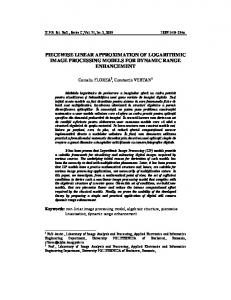
In Lemma 2 an intersection property of concave functions was explained. As it can be inferred from the proof of Lemma 3, ∆(x) ≥ 0. Therefore, with the results of Lemma 3 and Lemma 2, at this stage, Theorem 1 is given to find the points of maximum error in Γ, defined as emax = supx∈Γ ∆(x). Theorem 1: Consider a concave function f : Γ → R, Γ ⊂ R of class C 1 . Let the function be linearized around two points x1 , x2 ∈ Γ with lines h1 (x) and h2 (x) respectively. Furthermore, consider the point Pint = (xint , yint ) = {(x, y) | (x, y) ∈ S[h1 (x)]∩ S[h2 (x)]}. Then, the solution to the following maximization problem sup ∆(x) (30)

is a unit vector. Proof: f is concave, therefore − f is convex. The function h is also convex, because it is affine. Since the convexity property is kept under addition of convex functions [25], ∆(x) = h(x) − f (x) is convex. Since h is the linearization of f at x0 and f is concave, we have h ≥ f , according to the supporting hyperplane theorem [25]. This results in ∆(x) ≥ 0. In addition, because f (x0 ) = h(x0 ) implies ∆(x0 ) = 0, we can conclude that

x∈Γ

lies either on xint or at ∂ Γ = {q1 , q2 }. Proof: It can be recognized by Lemma 2 that x1 ≤ xint ≤ x2 . Furthermore x1 , x2 ∈ Γ, which implies that xint divides Γ into two sub-domains, each of which contains one of {x1 , x2 }. Let us denote the sub-domain containing x1 by Γx1 and the other one by Γx2 . In order to prove this theorem, Γ will be split into 4 different sub-domains, namely Γ2 , Γ1 , Γ3 and Γ4 , as Γ2 = conv(x1 , xint ), Γ1 = Γx1 \ Γ2 Γ3 = conv(x2 , xint ), Γ4 = Γx2 \ Γ3

(31)

where conv(·) denotes the convex hull of the points in the argument. Regarding the conditions of Lemma 3, the distance function ∆(x), from equation (8), can be represented as  ∆1 (x) = h1 (x) − f (x) , x ∈ Γx1 ∆(x) = (32) ∆2 (x) = h2 (x) − f (x) , x ∈ Γx2 In view of the fact that vx1 and vx2 are determined using

x0 = argmin ∆(x) x∈Γ

as the point of global minimum of ∆(x). Using the first order necessary condition for the points of minimum [25], we have Fig. 1.

∇∆(x0 ) = 0.

The intersection of h1 and h2 at Pint .

(29)

Furthermore, noting that −∆(x) is concave, Lemma 1 is used to say that ∆0 (x) is either increasing or remains stationary as

(28), as unit direction vectors at x1 and x2 respectively, the following 2 cases are investigated.

5

1) x ∈ Γ2 Γ3 S 2) x ∈ Γ1 Γ4 CASE 1. First, we consider x ∈ Γ2 . Let xΓ2 (p) = x1 + ε p, where p ∈ {p ∈ Z > 0 | p < pmax2 } with pmax2 defined such that xint = x1 + ε pmax2 . Using vx1 as a function of x, we have ∇∆1 (x) · vx1 (xΓ2 ) ≥ 0 by Lemma 3. Therefore, for ε sufficiently small, ∆1 (x1 ) ≤ ∆1 (x1 + ε), which is equivalent to ∆1 (xΓ2 (0)) ≤ ∆1 (xΓ2 (1)). Similarly, we have ∆1 (xΓ2 (1)) ≤ ∆1 (xΓ2 (2)), which using a sequence including 0 ≤ p ≤ pmax2 we reach the conclusion that ∆1 (xΓ2 (p)) ≤ ∆1 (xΓ2 (pmax2 )). In another word S

∆1 (x) ≤ ∆1 (xint ),

∀x ∈ Γ1 .

(33)

Likewise, defining xΓ3 (p) = x2 − ε p where p ∈ {p ∈ Z > 0 | p < pmax3 } with pmax3 defined as xint = x2 − ε pmax3 . Using the same idea, one can conclude that ∆2 (x) ≤ ∆2 (xint ),

∀x ∈ Γ2 .

(34)

CASE 2. In the second case, let x ∈ Γ1 . using Lemma 3 we have ∇∆1 (x) · vx1 (xΓ1 ) ≤ 0. Considering xΓ1 (p) = x1 − ε p where p ∈ {p ∈ Z > 0 | p < pmax1 } with pmax1 defined as q1 = x1 − ε pmax1 , we may write ∆1 (xΓ1 (0)) ≤ ∆1 (xΓ1 (1)). Using a sequence, similar to the argument in Case 1, we have ∆1 (x) ≤ ∆1 (q1 ),

∀x ∈ Γ3 .

(35)

Obviously, for x ∈ Γ4 , one can easily check that ∆2 (x) ≤ ∆2 (q2 ),

∀x ∈ Γ4 .

(36)

Equations (33), (34), (35) and (36) guarantee that an element from the set {xint , q1 , q2 } is indeed a solution to (30). The objective at each stage is to linearize the function at the points of maximum error occurring during the linearization. Theorem 1 ensures that after the first stage of approximation, the solution to (30) lies either on xint , or q1 , or q2 . If the first linearization occurs very close to q1 and q2 such that ∆(q1 ) ≤ edes and ∆(q2 ) ≤ edes , the solution to (30) will be xint . Therefore, xint is the next point at which f should be linearized (see the upper plot in Figure 2). Denoting this linearization by h3 , the second approximation stage is started as the point xint adopts a new notation x3 (see the lower plot in Figure 2). Updating the distance function ∆(x) using (8), the problem of approximating f is formalized with two parts, as to find 1) argmax ∆(x)

(37)

x1 ≤x≤x3

2) argmax ∆(x),

(38)

x3 ≤x≤x2

which are the points of maximum error. Since f is concave within x1 ≤ x ≤ x3 and x3 ≤ x ≤ x2 , Theorem 1 is then used to find the solution for (37) and (38). This process is continued as long as maxx∈Γ ∆(x) > edes . With all of the theoretical background that has been provided in this section, the algorithm for the intersection-based PWA approximation can be described in the next section. IV. A LGORITHMS In this section, the algorithms elaborating the intersectionbased PWA (IPWA) approximation for both concave/convex and continuous functions are introduced.

Fig. 2. The upper plot shows the primary epoch of the approximation while the lower plot provides the second epoch. Note that the superscripts reset at each epoch.

A. Concave/Convex Functions This algorithm is proposed for a concave function. If f is convex, − f is then considered. Problem 1: Consider a concave function f : Γ → R, where Γ ⊂ R. Find f¯ over the domain of f . 1) The primary linearization points are determined. The points are chosen at which the user needs zero error. As mentioned above, the primary linearization points are selected in accordance with the nature of the problem for which the IPWA being obtained is considered to serve. One can still add other initial points heuristically, like the points of zero curvature. This idea was originally suggested by Casselman and Rodrigues in reference [26], as the essential idea of the SLP method. Although the idea seems to improve the approximation, Example 4 shows a purely mathematical equation where setting the zero curvature point as a primary linearization point does not necessarily reduce the error. 2) Using Taylor series, the function f is linearized around all the points obtained in step 1. The produced linearization hyperplanes are denoted by hi (x), where i ∈ I = {1, 2, ..., Nu } and Nu is the number of linearization points at the uth loop. 3) Each two neighboring hyperplanes hi (x) will intersect with each other, resulting in a point. These points are (k) designated by Pint (x), where k ∈ K = {1, 2, ..., Nu2 } and

6

Nu2 is the number of the intersections in the uth loop. (k) 4) The projection of the all intersection points Pint on Γ is (k) denoted by xint . 5) Using Theorem 1 the points at which the local maximum errors occur are determined. According to this theorem, (1) (k) these points belong to the set M = {x1 , xint , ..., xint , x2 }. The global maximum is then obtained by updating ∆(x) using (8), and then evaluating ∆(x) for all the elements of M. Comparing the results, the value at which the global maximum error occurs and the error itself are found, as emax is set as xemax = argmax ∆(x) x∈M

emax = max ∆(x) x∈M

6) The stopping criterion is defined as emax ≤ edes

(39)

where edes is called desired error and is defined to be the maximum allowable error determined by the user. Then edes is compared with the value of emax , obtained in step 5. If the stopping criterion is met, the IPWA approximation is produced. Otherwise, the point of maximum error is given to step 2 for the next linearization stage. This loop is continued until the stopping criterion is satisfied.

The regions produced by both of the proposed algorithms are convex and have been defined in equation (4) in section III. V. A PPLICATIONS In this section the IPWA approximation algorithm is applied to four examples. The obtained IPWA models of Examples 1 to 3 are compared with the Lebesgue and the uniform grid PWA approximation techniques while Example 4 is compared with the SLP algorithm proposed by [26]. The normalized approximation error e¯max that is used for the comparison purpose is computed by emax , (40) e¯max = maxx∈Γ f (x) − minx∈Γ f (x) where f (x) is the exact function, and Γ is the domain of f . Example 1: A wheeled mobile robot (WMR) with a rigid structure is considered for a path following problem. The idea is to have the rover followed the y axis with zero heading. The WMR moves with a constant velocity V0 and is rotated by torque T exerted by an actuator, as shown in Figure 3.

B. Continuous Functions In this section, the function f is considered with only the continuity property. Despite the fact that such a function, that may not be concave nor convex, is rather difficult to tackle, many applications, including Examples 1 and 3, are neither concave nor convex. For this purpose, the IPWA algorithm for approximating continuous functions is given in this section. In this algorithm, the inflection points of f (x) are found first. The curvature of f at these points attains zero and the convexity of f changes. The set of inflection points are denoted by K = {xκ1 , xκ2 , · · · , xκq }. Therefore, function f can be split into q + 1 functions, as f1 (x), f2 (x), · · · , fq+1 (x), each being either convex or concave. For this aim, the initial linearization points are chosen to be the members of K . The initial linearization hyperplanes h1κ , h2κ , · · · , hqκ are then constructed using the Taylor series. Since each fi (x) possesses either the concavity/convexity property, the IPWA algorithm for concave/convex functions is, therefore, used to compute the IPWA approximation for each fi (x). The details of this method are summarized in the following algorithm. Problem 2: Consider a continuous function f : Γ → R, where Γ ⊂ R. Find f¯. 1) In the initial linearization stage, select the points from both categories: a) members of set K , and b) the reference point (if the approximation purpose is to solve a control synthesis problem). 2) Repeat steps 2 to 6 from section IV-A for f .

Fig. 3. Free body diagram of the WMR, where ψ is the heading, and V0 is the velocity of CG.

For simplification, we have assumed that the center of gravity is located in the mid point of the vehicle axle. This assumption is quite reasonable since the driver motors, which make the major contribution to the vehicle wight, are usually mounted on the top of the axle position. Denoting x1 = y, ˙ the equations of motion for this problem can x2 = ψ, x3 = ψ, be written as x˙1 =V0 sin x2 x˙2 =x3 x˙3 =Iz T,

(41a) (41b) (41c)

where Iz is the WMR moment of inertia in the z axis. It is recognized that fnl (x) = [ f1 (x2 ), 0, 0]T , comparing (41) with (1). Therefore the IPWA algorithm can be used to obtain the IPWA approximation for f1 (x2 ) = V0 sin(x2 ). The function f1 (x2 ) with its IPWA approximation is plotted in Figure 4. The upper plot is associated with the 2nd iteration while the lower plot indicates the 3rd iteration of the proposed algorithm. Due to the symmetry of the sine function, points (1) (2) (3) (2) xint = −2.136, xint = −1.0, xint = 1.0 and xint = 2.136 have the same value for the approximation error. Therefore, the

7

TABLE I T HE SUMMARY OF PIECEWISE AFFINE APPROXIMATION FOR f1 (x2 ) = sin x2 .

1.0 0.8

Normalized Approximation Error (e¯max ) of f1 (x2 ) N UMBER OF IPWA L EBESGUE PWA UG PWA R EGIONS n A PPROX . A PPROX . A PPROX . 3 0.2854 0.3536 0.2182 4 NA 0.1036 0.0668 5 0.0793 NA 0.0909 7 NA 0.0849 0.0479 8 NA 0.0581 0.0244 9 0.0229 NA 0.0292 11 NA 0.0504 0.0140 12 NA 0.0398 0.0124 13 0.0191 NA 0.0144 15 NA 0.0359 0.0108 16 NA 0.0302 0.0074 17 0.0067 NA 0.0084 19 NA 0.0279 0.0065 20 NA 0.0244 0.0040 21 0.0054 NA 0.0056

0.6

f1 (x2 )

0.4 0 −0.2 −0.4 −0.6 −0.8 −1.0 −π

−π/2

0 x2

π/2

π

−π/2

0 x2

π/2

π

1.0 0.8 0.6

f1 (x2 )

0.4

function is linearized around all of the intersection points in the next loop of the algorithm. The summary of the approximation is found in Table I, where the proposed algorithm is compared to the uniform grid and the Lebesgue PWA approximation methods. As it can be seen, the approximation iteration is done until e¯max = 0.0054 with 21 regions. As mentioned earlier with the numerical values, the symmetry of the sine function for the IPWA algorithm may cause several points with the same value of error in each linearization stage, hence the number of regions may increase by more than 1 region per iteration. This is the reason we marked ‘NA’ in the second column of Table I. A similar phenomenon was encountered with the Lebesgue approximation applied to the sine function. Consequently, the comparison of each methodology can be accomplished using the numerical values obtained with the uniform grid technique. It can be seen that the e¯max of the uniform grid PWA model is less than the same parameter for the Lebesgue model in each epoch. On the other hand, smaller values for e¯max are obtained with the IPWA model compared to the uniform grid model. Example 2: Consider a rigid airfoil that has two degrees of freedom: plunging along the h direction, and pitching in α. The authors of reference [27] have summarized the dynamics of the wing fluctuation using a linear and an angular springs, which are shown in Figure 5. By doing so, the nonlinear aeroelastic behavior of the wing can be modeled by a polynomial function of the pitch angle. ˙ α] ˙ T = [x1 , x2 , x3 , x4 ]T as the system states, Denoting [h, α, h, the governing equations are written as x˙ = AF x + fF (x) + BF u,

0.2

0.2 0 −0.2 −0.4 −0.6 −0.8 −1.0 −π

Fig. 4. IPWA approximation of the f1 (x2 ) = sin (x2 ). The upper plot is the approximation with 5 regions. The approximation has been refined in the lower figure by linearizing the intersection points, which are plotted with squares.

Fig. 5.

Simplified aeroelastic model of the aircraft wing.



 0.0 0.0   0.0 0.0  BF =   −7606.8 −7642.6  , 14250 9021.9 and 

 0   0  fF (x) =   K¯ α (x2 )  , K¯ α (x2 )

(42) with

where

K¯ α (x2 ) =2.82x2 − 62.322x22 + 3709.71x23 

 0.0 0.0 1.0 0.0   0.0 0.0 0.0 1.0  AF =   −293.27 −100.59 −5.9027 −0.40542  , 1885.9 743.79 34.728 2.4687

− 24195.6x24 + 48756.954x25 that are taken from [27]. K¯ α (x2 ) is a function of only one variable x2 , which allows us to use the IPWA algorithm to compute its PWA approximation. The summary of the IPWA

8

algorithm applied to the continuous function K¯ α (x2 ) for x2 ∈ (−π/6, π/6) is given in Table II. The normalized error e¯max is computed according to (40). Figure 6 shows two consecutive (3) iterations of the IPWA algorithm. Point xint = −0.3434 has the maximum error of approximation in the 3rd iteration (upper plot). This point is thus chosen to linearize the function K¯ α (x2 ), resulting in a finer PWA approximation (lower plot). Looking at Table II, one can concludes that the Lebesgue model has the least error for 3 regions while for more than 3 regions the IPWA is shown to produce better results. TABLE II T HE SUMMARY OF PIECEWISE AFFINE APPROXIMATION FOR K¯ α (x2 ) Normalized N UMBER OF R EGIONS n 3 4 5 6 7 9

Approximation Error (e¯max ) of K¯ α (x2 ) IPWA L EBESGUE PWA UG PWA A PPROX . A PPROX . A PPROX . 0.3337 0.2492 0.3867 0.1113 0.1658 0.3010 0.0731 0.1242 0.2285 0.0483 0.0992 0.1684 0.0371 0.0825 0.1187 0.0195 0.0710 0.0423

Fig. 7. Two-gene regulatory network. x1 and x2 represent mRNAs concentration while x3 and x4 stand for the protein product concentration of genes A and B, respectively. This figure is adapted from [9].

concentration of all genes A and B, respectively, the governing state space equations of the two-gene regulatory network is described by 2000

x˙1 =α1 σn (x4 ) − β1 x1 x˙2 =α2 x1 − β2 x2 x˙3 =α3 σ p (x2 ) − β3 x3 x˙4 =α4 x3 − β4 x4

¯ α (x2 ) K

1500 1000 500 0 −π/6

−π/12

0 x2

π/12

π/6

θnκ + x4κ xκ σ p (x2 ) = κ 2 κ , θ p + x2

1500 ¯ α (x2 ) K

where σn and σ p are the transcriptional regulation functions depending on the concentrations of the protein products, according to [28] and [9]. These functions for a two-gene network problem may take the form of σn (x4 ) =

2000

1000 500 0 −π/6

(43a) (43b) (43c) (43d)

−π/12

0 x2

π/12

π/6

Fig. 6. IPWA approximation of the K¯ α (x2 ). The upper plot is the approximation at the 3rd iteration while the lower plot is associated with the 4th iteration of the algorithm.

Example 3: A set of cell DNAs that interact through their RNA and their protein products is called a gene regulatory network. Based on the interactive regulation of genes, a genetic network is produced, which describes the behavior of organisms, according to [28]. The two-gene regulation network is schematically shown in Figure 7. Denoting x1 and x3 as the concentration of messenger RNAs (mRNAs), as well as x2 and x4 as the protein products

(44)

θnκ

with θn = 0.20, θ p = 0.19 and taken from [9], as     α1 0.95  α2   1.23       α3  =  0.86  , α4 1.43

(45)

κ = 4. All the constants are 

  β1 0.90  β2   1.31 =   β3   0.83 β4 2.60

  . 

Using the IPWA algorithm, functions σn (x4 ) and σ p (x2 ) are approximated for several desired errors. The Lebesgue approximation and the uniform grid techniques are also used to find the PWA model of these functions. The approximation error of all of the mentioned techniques are presented in Tables III and IV. For as low number of regions as three, the Lebesgue algorithm is shown to be most accurate. As the number of the regions is increased, the IPWA provides higher accuracy with respect to the other techniques. Example 4: The last example for modeling of nonlinear systems with IPWA method consists of the mathematical

9

TABLE III T HE SUMMARY OF PIECEWISE AFFINE APPROXIMATION FOR σn (x4 ) Normalized N UMBER OF R EGIONS n 3 4 5 6 7 8 9 10 11

Approximation Error (e¯max ) of σn (x4 ) IPWA L EBESGUE PWA UG PWA A PPROX . A PPROX . A PPROX . 0.1738 0.1575 0.2083 0.0721 0.1167 0.2283 0.0667 0.0922 0.1912 0.0405 0.0760 0.1364 0.0259 0.0644 0.0907 0.0217 0.0558 0.0598 0.0196 0.0492 0.0439 0.0135 0.0439 0.0419 0.0109 0.0396 0.0464

R EFERENCES

TABLE IV T HE SUMMARY OF PIECEWISE AFFINE APPROXIMATION FOR σ p (x2 ) Normalized N UMBER OF R EGIONS n 3 4 5 6 7 8 9 10 11

Approximation Error (e¯max ) of σ p (x2 ) IPWA L EBESGUE PWA UG PWA A PPROX . A PPROX . A PPROX . 0.1745 0.1589 0.2001 0.0721 0.1178 0.2289 0.0672 0.0933 0.2043 0.0406 0.0771 0.1529 0.0262 0.0655 0.1052 0.0217 0.0568 0.0705 0.0196 0.0556 0.0479 0.0136 0.0447 0.0436 0.0109 0.0403 0.0447

function  4 f (x) = x + 4−1/3 − x − 4−4/3 ,

∀x ∈ Γ,

unicycle, the aeroelastic model of the aircraft wing, and the two-gene regulatory network. The approximation error of the intersection-based PWA model of the examples was compared with the Lebesgue [9], uniform grid [7], and the SLP [26] PWA models. Future work may involve study of the PWA approximation of functions of two or more variables.

(46)

where Γ = (−2, 1). The specific feature of this function is that it has a zero curvature point at xzc = 4−1/3 , which is not an inflection point. Therefore, the SLP algorithm picks xzc as a member of the set of linearization points (SLP). The IPWA algorithm in contrast, does not linearize the function f at such point. Table V gives the normalized approximation error of PWA approximation of f by both the SLP and the IPWA algorithms. Although the error for both models with 2, 4 and 8 regions is the same, the IPWA model has smaller values of error with 3 and 5 regions. TABLE V T HE SUMMARY OF PIECEWISE AFFINE APPROXIMATION FOR f (x) Normalized Approximation Error (e¯max ) of f (x) Given in Equation (46) N UMBER OF IPWA SLP PWA R EGIONS n A PPROX . A PPROX . 2 1.0000 1.0000 3 0.3401 0.5970 4 0.3037 0.3037 5 0.1469 0.1888 6 0.0896 0.0896

VI. C ONCLUSION In this paper, the intersection-based algorithm for approximation of functions of one variable was developed. Using the algorithms provided in section IV, PWA models can be constructed for a wide range of nonlinear functions, where the nonlinearity is a function of only one state. Finally the method was successfully applied to the path following

[1] Mikael Johansson. Piecewise Linear Control Systems. Springer-Verlag, Berlin, first edition, 2003. [2] L. Rodrigues and J.P. How. Synthesis of piecewise-affine controllers for stabilization of nonlinear systems. Proceedings of the 42nd IEEE Conference on Decision and Control, 3:2071–2076, 2003. [3] L. Rodrigues and S. Boyd. Piecewise-affine state feedback for piecewiseaffine slab systems using convex optimization. Systems & Control Letters, 54:835–853, 2005. [4] S. Casselman and L. Rodrigues. Piecewise affine modeling of a micro air vehicle using voronoi partitions. In Proceedings of the European Control Conference, pages 3857–3862, 2009. [5] A. Cantoni. Optimal curve fitting with piecewise linear functions. IEEE Transactions on Computers, C-20:59–67, January 1971. [6] I. Tomek. Two algorithms for piecewise-linear continuous approximation of functions of one variable. IEEE Transactions on Computers, C24:445–448, April 1974. [7] P. Julian, A. Desages, and O. Agamennoni. High-level canonical piecewise linear representation using a simplicial partition. IEEE Transactions on Circuits and Systems I: Fundamental Theory and Applications, 46:1057–7122, April 1999. [8] Richard E. Groff, Pramod P. Khargonekar, and Daniel E. Koditschek. A local convergence proof for the MINVAR algorithm for computing continuous piecewise linear approximations. SIAM Journal of Numerical Analysis, 41(3):983–1007, 2003. [9] S. Azuma, J. Imura, and T. Sugie. Lebesgue piecewise affine approximation of nonlinear systems. Nonlinear Analysis: Hybrid Systems, 4(1):92– 102, 2010. [10] Marco Storace and Oscar De Feo. Piecewise-linear approximation of nonlinear dynamical systems. IEEE Transactions on Circuits and Systems, Vol. 51(No. 4):830–842, 2004. [11] Jorge M. Gonc¸alves, Alexandre Megretski, and Munther A. Dahleh. Global analysis of piecewise linear systems using impact maps and surface lyapunov functions. IEEE Transactions on Automatic Control, Vol. 48(No. 12):2089–2106, 2003. [12] E. Asarin, T. Dang, and A. Girard. Hybrid Systems: Computation and Control, pages 20–35. Springer, 2003. [13] Gang Feng. Controller design and analysis of uncertain piecewise-linear systems. IEEE Transactions on Circuits and Systems - I: Fundamental Theory and Applications, Vol. 49(No. 2):224–232, 2002. [14] Luis Rodrigues and Jonathan P. How. Automated Control Design for a Piecewise-Affine Approximation of a Class of Nonlinear Systems. In Proceedings of the American Control Conference, pages 3189–3194, 2001. [15] Wei Yue, Luis Rodrigues, and Brandon Gordon. Piecewise-affine control of a three DOF helicopter. In Proceedings of the 2006 American Control Conference, pages 3924–3929, 2006. [16] Daniele Corona and Bart De Schutter. Adaptive cruise control for a SMART car: A comparison benchmark for MPC-PWA control methods. IEEE Transactions on Control Systems Technology, Vol. 16(Number 2):365–372, 2008. [17] G. Ferrari-Trecate, M. Muselli, D. Liberati, and M. Morari. A clustering technique for the identification of piecewise affine systems. Automatica, 39(2):205–217, 2003. [18] A. Bemporad and M. Morari. Control of systems integrating logic, dynamics, and constraints. AUTOMATICA-OXFORD-, 35:407–428, 1999. [19] C. Tomlin, I. Mitchell, and R. Ghosh. Safety verification of conflict resolution manoeuvres. Intelligent Transportation Systems, IEEE Transactions on, 2(2):110–120, 2001. [20] R. Ghosh, A. Tiwari, and C. Tomlin. Automated symbolic reachability analysis; with application to delta-notch signaling automata. Hybrid Systems: Computation and Control, pages 233–248, 2003. [21] S.I. Azuma and J.I. Imura. Polynomial-time probabilistic controllability analysis of discrete-time piecewise affine systems. Automatic Control, IEEE Transactions on, 52(11):2029–2046, 2007.

10

[22] S. Azuma and J. Imura. Polynomial-time probabilistic observability analysis of sampled-data piecewise affine systems. In Decision and Control, 2005 and 2005 European Control Conference. CDC-ECC’05. 44th IEEE Conference on, pages 6644–6649. IEEE, 2005. [23] Behzad Samadi and Luis Rodrigues. Extension of local linear controllers to global piecewise affine controllers for uncertain non-linear systems. International Journal of Systems Science, 39(9):867–879, 2008. [24] H.L. Royden. Real Analysis. MACMILLAN, second edition, 1968. [25] David G. Luenberger and Yinyu Ye. Linear and Nonlinear Programming. Springer, third edition, 2008. [26] S. Casselman and L. Rodrigues. A new methodology for piecewise affine models using voronoi partitions. In Proc. 48th IEEE Conference on Decision and Control and 28th Chinese Control Conference, pages 3920 –3925, 2009. [27] S. Afkhami and H. Alighanbari. Nonlinear control design of an airfoil with active flutter suppression in the presence of disturbance. IET Control Theory Appl., 1(6):1638–1649, November 2007. [28] A. Mochizuki. An analytical study of the number of steady states in gene regulatory networks. Journal of Theoretical Biology, 236(3):291–310, 2005.