imated steady-state solution, it does not exploit the piece- wise switched nature of power electronics circuits. Power electronics circuits are defined by a set of ...
Wavelet-Based Piecewise Approximation of Steady-State Waveforms for Power Electronics Circuits Kam C. Tam, Siu Chung Wong and Chi K. Tse Department of Electronic and Information Engineering, Hong Kong Polytechnic University, Hong Kong http://chaos.eie.polyu.edu.hk
Abstract— Wavelet transform has been found very suitable for approximating steady-state waveforms of power electronics circuits. However, the time-domain piecewise property of power electronics circuits has not been fully exploited to maximize computational efficiency. In this paper, instead of applying one wavelet approximation to the whole period, several wavelet approximations are applied in a piecewise manner to fit the whole waveform. This new wavelet-based piecewise approximation approach can provide very accurate and efficient solution, with much less number of wavelet terms, for approximating steadystate waveforms of power electronics circuits.
I. I NTRODUCTION Steady-state voltage and current waveforms of critical components in power electronics circuits often represent an important part of design information for ensuring reliable operation, since excessive voltage and current stresses can be detrimental to certain semiconductor devices. Traditional methods, such as brute-force transient simulation, for obtaining the steady-state waveforms are usually time consuming and may suffer from numerical instabilities, especially for power electronics circuits consisting of slow and fast variations in different parts of the same waveform. Wavelets have been shown to be highly suitable for describing waveforms with fast changing edges embedded in slowly varying backgrounds [1], [2]. A systematic algorithm for approximating steadystate waveforms arising from power electronics circuits using Chebyshev-polynomial wavelets has been proposed by Liu, Tse and Wu [3]. Moreover, power electronics circuits are piecewise varying in the time domain. Thus, approximating a waveform with one wavelet approximation (i.e., using one set of wavelet functions and hence one set of wavelet coefficients) is rather inefficient as it may require an unnecessarily large wavelet set. In this paper, we propose a piecewise approach to solving the problem, using as many wavelet approximations as the number of switch states. The method yields an accurate steadystate waveform description with much less number of wavelet terms. The paper is organized as follows. A procedure for approximating steady-state waveforms of piecewise switched systems is described in Section II. In Section III, we evaluate and compare the effectiveness of the proposed piecewise wavelet approximation with that of the standard wavelet approximation. Finally, we give the conclusion in Section IV.
0-7803-8834-8/05/$20.00 ©2005 IEEE.
2490
II. WAVELET- BASED P IECEWISE A PPROXIMATION It has been shown that wavelet approximation [3] can be useful for approximating steady-state waveforms of power electronics circuits as it takes advantage of the inherent nature of wavelets in describing fast edges embedded in slowly moving backgrounds. In most cases, power electronics circuits can be represented by a time-varying state-space equation x˙ = A(t)x + U (t)
(1)
where x is the m-dim state vector, A(t) is an m × m timevarying matrix, and U is the input function. Specifically we write ⎤ ⎡ a11 (t) a12 (t) · · · a1m (t) ⎥ ⎢ .. .. .. .. (2) A(t) = ⎣ ⎦ . . . . am1 (t) am2 (t) · · · amm (t) and
⎤ u1 (t) ⎥ ⎢ .. U (t) = ⎣ ⎦. . um (t) ⎡
(3)
In the steady state, the solution satisfies x(t) = x(t + T ) for 0 ≤ t ≤ T
(4)
where T is the period. For an appropriate translation and scaling, the boundary condition can be mapped to the closed interval [−1, 1] x(+1) = x(−1) (5) Assume that the basic time-invariant approximation equation is xi (t) = K Ti Ψ(t), for − 1 ≤ t ≤ 1 and i = 1, 2, · · · , m (6) where Ψ(t) is any wavelet basis of size 2 n+1 + 1 (n being the wavelet level) [3], [4] 1 , K Ti = [ki,0 · · · ki,2n+1 ] is a coefficient vector of dimension 2 n+1 +1, which is to be found. The wavelet transformed equation of (1) is KDΨ = A(t)KΨ + U (t)
(7)
1 The construction of wavelet basis has been discussed in detail in Liu et al. [3] and more formally in Frazier [4]. For more details on polynomial wavelets, see Kilgore et al. [5] and Fisher et al. [6].
This equation can be easily solved by applying an appropriate interpolation technique or via direct numerical convolution [7], which generates approximate solutions for the steady state. Although this standard algorithm provides a well approximated steady-state solution, it does not exploit the piecewise switched nature of power electronics circuits. Power electronics circuits are defined by a set of linear differential equations governing the dynamics for different intervals of time corresponding to different switch states. In the following, we propose a new wavelet approximation algorithm specifically for treating power electronics circuits. For each interval (switch state), we can find a wavelet representation. Then, a set of wavelet representations for all switch states can be “glued” together to give a complete steady-state waveform. Formally, consider a p-switch-state converter. We can write the describing differential equation, for switch state j as
S3
S4
S5
0
t
0
1
Fig. 1.
x˙j = Aj x + U j for j = 1, 2, · · · , p
S2
S1 H
t2
t3
t4
T
A single pulse waveform consisting of 5 switch states.
(8) 15
where Aj is a time invariant matrix at state j. Equation (8) is the piecewise state equation of the system. In the steady state, the solution satisfies the following boundary conditions xj−1 (Tj−1 ) = xj (0) for j = 2, 3, · · · , p
10
5
(9)
0 −1
and
−0.8
−0.6
−0.4
−0.2
0
0.2
0.4
0.6
0.8
1
0.2
0.4
0.6
0.8
1
(a)
x1 (0) = xp (Tp )
(10)
15
�p
10
where Tj is the time duration of state j and j=1 Tj = T . Thus, mapping all switch states to the close interval [−1, 1] in the wavelet space, the basic approximate equation becomes
5 0 −5 −10
xj,i (t) =
K Tj,i Ψ(t),
for − 1 ≤ t ≤ 1
(11) K Tj,i
= with j = 1, 2, · · · , p and i = 1, 2, · · · , m, where [k1,i,0 · · · k1,i,2n+1 , k2,i,0 · · · k2,i,2n+1 , kj,i,0 · · · kj,i,2n+1 ] is a coefficient vector of dimension (2 n+1 + 1) × p, which is to be found. As mentioned previously, the state equation is transformed to the wavelet space and then solved by using interpolation. Finally, all the coefficients necessary for generating approximate solutions for each switch state for the steady-state system are obtained. It should be noted that the wavelet-based piecewise method can be further enhanced for approximating steady-state solution using different wavelet levels for different switch states. Essentially, wavelets of high levels should only be needed to represent waveforms in switch states where high-frequency details are present. By using different choices of wavelet levels for different switch states, solutions can be obtained more quickly. This can be done by modifying the procedure explained in this section. III. S IMULATIONS AND E VALUATIONS Results can be evaluated using the mean relative error (MRE) and mean absolute error (MAE), which are defined
2491
−15 −20 −1
−0.8
−0.6
−0.4
−0.2
0 (b)
Fig. 2. Approximated pulse waveforms. Solid line is standard wavelet approximated waveform using wavelets of levels from −1 to 5 and dashed line is the piecewise wavelet approximated waveforms using wavelets of levels from −1 to 1. (a) Switch states 2 and 4 with rising and falling times both equal to 5 percent of the period; (b) switch states 2 and 4 with rising and falling times both equal to 1 percent of the period.
as MRE =
N 1 � xˆi − xi N i=1 xi
(12)
MAE =
N 1 � |ˆ xi − xi | N i=1
(13)
where N is the total number of points sampled along the interval [−1, 1] for error calculation. In the following, we use uniform sampling (i.e., equal spacing) with N = 1001, including boundary points. Example 1: A Single Pulse Waveform Consider a single pulse waveform shown in Fig. 1. It is considered here as an example of a waveform that cannot be
D Rl
Lm im
E
+ –
Ll il
Rm
C
ideal transformer
R
Lm
Rm C
R
im E
+ –
+ Cs vs –
+ vo –
Lm
Rs
+ Cs vs –
Rm C
im E
Ll il
(a) Fig. 3.
Rl
Rl
+ vo –
+ –
R
+–
– vo +
RD V f
Ll il
+ Cs vs –
(b)
(c)
(a) Flyback converter model with transformer leakage inductance and device parasitic capacitance; (b) on-time model; (c) off-time model. TABLE I
efficiently approximated by the standard wavelet algorithm. The waveform consists of five switch states (S1 to S5) and the corresponding state equations are given by (8), where A j and U j are given specifically as ⎧ 0 if 0 ≤ t < t1 ⎪ ⎪ ⎪ ⎨ 0 if t1 ≤ t < t2 Aj = 1 if t2 ≤ t < t3 (14) ⎪ ⎪ 0 if t ≤ t < t ⎪ 3 4 ⎩ 0 if t4 ≤ t ≤ T . and
⎧ 0 ⎪ ⎪ ⎪ ⎨ H/(t2 − t1 ) U j = −H ⎪ ⎪ ⎪ ⎩ −H/(t4 − t3 ) 0
if if if if if
0 ≤ t < t1 t 1 ≤ t < t2 t 2 ≤ t < t3 t 3 ≤ t < t4 t4 ≤ t ≤ T .
(15)
where H is the amplitude (see Fig. 1). Switch states 2 (S2) and 4 (S4) correspond to the rising edge and falling edge, respectively. Obviously, when the widths of rising and falling edges are small, the standard wavelet method cannot provide a satisfactory approximation for the system unless very high wavelet levels are used. Figs. 2 (a) and (b) show the approximated pulse waveforms using our waveletbased piecewise method and the standard wavelet method for two different choices of wavelet levels with different widths of rising and falling edges. This example clearly shows the benefits of the wavelet-based piecewise approximation using separate sets of wavelet coefficients for the different switch states. Example 2: Flyback Converter with Parasitic Ringings Next, we consider the flyback converter circuit, which is shown in Fig. 3 (a). This is a realistic model as the parasitic capacitance across the switch and leakage inductance of the transformer are deliberately included. The operation is simplified to two switch states as follows. When the switch is turned on, current flows through the magnetizing inductance L m and the leakage inductance L l , with the transformer secondary opened and the diode not conducting. When the switch is turned off, the transformer secondary conducts through the diode, clamping the primary voltage (i.e., voltage across L m ) to the output network (assuming a 1:1 turns ratio). Thus, L m
2492
C OMPONENT AND PARAMETER VALUES FOR S IMULATION . Component/Parameter Magnetizing (storage) inductance, Lm Leakage inductance, Ll Equivalent parallel resistance of transformer primary, Rm Output capacitance, C Load resistance, R Input voltage, E Diode forward drop, Vf Switching period, T On-time, TD Equivalent loop resistance, Rl Switch on-resistance, RS Switch capacitance, CS Diode on-resistance, RD
Value 0.4 mH 1 µH 1 MΩ 0.1 mF 12.5 Ω 16 V 0.8 V 100 µs 45 µs 0.4 Ω 0.001 Ω 200 nF 0.001 Ω
discharges through the transformer primary, while the leakage Ll and the parasitic capacitance C s form a damped resonant loop around the input voltage source. Figs. 3 (b) and (c) show the detailed circuit models for the on-time and off-time durations, respectively. The state equation of this converter is given by x˙ = A(t)x + U (t) (16) where x = [im il vs vo ]T , and A(t) and U (t) are given by A(t) U (t)
= A1 (1 − s(t)) + A2 s(t) = U 1 (1 − s(t)) + U 2 s(t)
with s(t) defined as ⎧ for 0 ≤ t ≤ TD ⎨0 for TD ≤ t ≤ T s(t) = 1 ⎩ s(t − T ) for all t > T .
(17) (18)
(19)
and the U ’s and A’s being derivable from the circuit topologies. The parameters for simulation are listed in Table I. We will compare the approximated waveforms of the switch voltage using the piecewise approach and the standard wavelet method. Figs. 4 (a) and (b) show the approximated waveforms using the piecewise and standard wavelet methods for two different choices of wavelet levels. As expected, the new piecewise technique gives more accurate results with wavelets of relatively low levels. Since the waveform contains a substantial portion
TABLE II C OMPARISION OF MAE S . A LL WAVELETS UP TO LEVELS 4, 5, 6, 7 AND 8 ARE USED FOR APPROXIMATING THE SWITCH VOLTAGE IN THE FLYBACK
60 v (V) s 40
CONVERTER USING THE STANDARD AND PROPOSED PIECEWISE METHODS . 20
Wavelet levels −1 −1 −1 −1 −1
to to to to to
Number of wavelets
4 5 6 7 8
33 65 129 257 513
MAE for vs (standard) 2.581651 1.636094 1.354323 0.971359 0.540244
0
MAE for vs (piecewise) 0.844064 0.386680 0.340025 0.313124 0.298731
−20 −1
−0.8
−0.6
−0.4
−0.2
0
0.2
0.4
0.6
0.8
1
0.2
0.4
0.6
0.8
1
0 (c)
0.2
0.4
0.6
0.8
1
0
0.2
0.4
0.6
0.8
1
(a) 60 vs(V) 40
60
20 v (V) s
40
0
20
−20 −1
−0.8
−0.6
−0.4
−0.2
0 (b)
0 60 v (V)
−20 −1
−0.8
−0.6
−0.4
−0.2
0
0.2
0.4
0.6
0.8
1
s
40
(a) 20
60 vs(V) 40
0
20
−20 −1
−0.8
−0.6
−0.4
−0.2
−0.8
−0.6
−0.4
−0.2
0 60 −20 −1
vs(V) −0.8
−0.6
−0.4
−0.2
0
0.2
0.4
0.6
0.8
1
40
(b)
Fig. 4. Switch voltage waveforms of flyback converter. Solid line is waveform from wavelet-based piecewise approximation, dashed line is waveform from SPICE simulation and dot-dashed line is waveform using standard wavelet approximation, (a) using wavelets of levels from −1 to 4; (b) using wavelets of levels from −1 to 5.
20
0
−20 −1
(d)
where the value is near zero, we use the mean absolute error (MAE) for evaluation. From Table II, the result clearly verifies the advantage of using the proposed wavelet-based piecewise method. Inspecting the two switch states of the flyback converter, it is obvious that switch state 2 (off-time) is rich in high-frequency details, and therefore should be approximated with wavelets of higher levels. Fig. 5 shows the approximated waveforms with different choices of wavelet levels for switch states 1 (on-time) and 2 (off-time). IV. C ONCLUSION In this paper, a wavelet-based piecewise approximation method for finding steady-state waveforms of power electronics circuits has been proposed. Compared to the standard wavelet approximation, the proposed piecewise approach is more computational efficient and accurate, using much less wavelet coefficients and involving wavelets of lower levels. ACKNOWLEDGMENT This work was supported by a research grant provided by The Hong Kong Polytechnic University (Project A-PD68).
2493
Fig. 5. Switch voltage waveforms of flyback converter. Dashed line is waveform from SPICE simulation. Solid line is waveform using wavelet-based piecewise approximation. Two different wavelet levels, shown in brackets, are used for approximating switch states 1 and 2, respectively, (a) (3,4) with MAE = 1.041172; (b) (3,5) with MAE = 0.679942; (c) (4,5) with MAE = 0.480091; and (d) (5,6) with MAE = 0.387399.
R EFERENCES [1] E. Wernekinck, H. Valenzuela, and I. Anfossi, “On the analysis of power electronics circuits waveforms with wavelets,” Proc. Power Conversion Conf., pp. 544–549, 1993. [2] I. Daubechies, “Time-frequency localization operators: a geometric phase space approach,” IEEE Trans. Inform.Theory, vol. 34, pp. 605– 612, 1988. [3] M. Liu, C. K. Tse, and J. Wu, “A wavelet approach to fast approximation of steady-state waveforms of power electronics circuits,” Int. J. Circuit Theory Appl., vol. 31, no. 6, pp. 591–610, November 2003. [4] M. W. Frazier, An Introduction to Wavelets Through Linear Algebra, New York: Springer-Verlag, 1999. [5] T. Kilgore and J. Prestin, “Polynomial wavelets on the interval,” Constructive Approximation, vol. 12, pp. 95–110, 1995. [6] B. Fisher and J. Prestin, “Wavelets based on orthogonal polynomials,” Math. of Computation, vol. 66, no. 220, pp. 1593–1618, 1997. [7] K. C. Tam, S. C. Wong, and C. K. Tse, “A wavelet approach to finding steady-state power electronics waveforms using discrete convolution,” Int. Symp. Nonlinear Theory and Appl., (NOLTA’2004), Fukuoka, Japan, November-December 2004.