4.2 Display style math, with examples . .... command. For example, suppose I
wanted to underline a title in the following sentence: “Tolstoy wrote War and
Peace.
Introduction to LATEX 2ε by W. Ethan Duckworth Loyola College, Fall 2006
I wrote this guide to answer some basic questions. What is TEX? What is LATEX? Why would I want to use them? How do I use them? Are there any other interesting tidbits I should know? I hope this document is about as short as possible while accomplishing these goals.
Contents 1 What are TEX and LATEX?
1
2 Why would I want to use LATEX? 2.1 Mathematics . . . . . . . . . . . . . . . . . . . . 2.2 Logically structured documents . . . . . . . . . . 2.3 The virtue of languages . . . . . . . . . . . . . . 2.4 Perfection (and some interesting tidbits promised 2.5 Who is LATEX not for? . . . . . . . . . . . . . . . 2.6 Formatting and abstract markup . . . . . . . . .
. . . . . . . . . . . . above) . . . . . . . .
. . . . . .
. . . . . .
. . . . . .
. . . . . .
. . . . . .
. . . . . .
. . . . . .
. . . . . .
. . . . . .
. . . . . .
. . . . . .
. . . . . .
3 All right all ready, I’m dying to use it. But how? 4 How do I produce math formulas? 4.1 Math mode . . . . . . . . . . . . . . 4.2 Display style math, with examples . 4.3 Words in math mode . . . . . . . . . 4.4 Trigonometric and similar functions 4.5 Lining it up: tables and arrays . . . 4.6 Matrices . . . . . . . . . . . . . . . . 4.7 Lining up equations . . . . . . . . .
2 2 2 3 3 4 4 5
. . . . . . .
. . . . . . .
. . . . . . .
. . . . . . .
. . . . . . .
. . . . . . .
. . . . . . .
. . . . . . .
. . . . . . .
. . . . . . .
. . . . . . .
. . . . . . .
. . . . . . .
. . . . . . .
. . . . . . .
. . . . . . .
. . . . . . .
. . . . . . .
. . . . . . .
. . . . . . .
. . . . . . .
7 7 8 10 11 11 12 13
5 How do I do other word processor stuff ? 5.1 Default font size . . . . . . . . . . . . . . 5.2 Margins . . . . . . . . . . . . . . . . . . . 5.3 Line spacing . . . . . . . . . . . . . . . . . 5.4 Ending paragraphs and sentences . . . . . 5.5 Ending lines . . . . . . . . . . . . . . . . . 5.6 Justification and spacing of paragraphs . . 5.7 Centering . . . . . . . . . . . . . . . . . . 5.8 Spacing . . . . . . . . . . . . . . . . . . . 5.9 Quotation marks . . . . . . . . . . . . . . 5.10 Fonts . . . . . . . . . . . . . . . . . . . . . 5.11 Some title pages . . . . . . . . . . . . . . 5.12 Special symbols . . . . . . . . . . . . . . . 5.13 Lists . . . . . . . . . . . . . . . . . . . . . 5.14 Environments . . . . . . . . . . . . . . . . 5.15 User commands and environments . . . . 5.16 Packages . . . . . . . . . . . . . . . . . . . 5.17 Theorems, definitions, examples, etc . . .
. . . . . . . . . . . . . . . . .
. . . . . . . . . . . . . . . . .
. . . . . . . . . . . . . . . . .
. . . . . . . . . . . . . . . . .
. . . . . . . . . . . . . . . . .
. . . . . . . . . . . . . . . . .
. . . . . . . . . . . . . . . . .
. . . . . . . . . . . . . . . . .
. . . . . . . . . . . . . . . . .
. . . . . . . . . . . . . . . . .
. . . . . . . . . . . . . . . . .
. . . . . . . . . . . . . . . . .
. . . . . . . . . . . . . . . . .
. . . . . . . . . . . . . . . . .
. . . . . . . . . . . . . . . . .
. . . . . . . . . . . . . . . . .
. . . . . . . . . . . . . . . . .
. . . . . . . . . . . . . . . . .
. . . . . . . . . . . . . . . . .
. . . . . . . . . . . . . . . . .
18 18 18 19 19 21 21 22 22 25 25 27 27 28 30 32 34 35
6 Fancier stuff 6.1 References within document . . . . 6.2 Bibliography and citations . . . . . 6.3 Color . . . . . . . . . . . . . . . . . 6.4 Conditional commands . . . . . . . 6.5 Block comments with conditionals 6.6 Importing graphics . . . . . . . . . 6.7 Floating figures . . . . . . . . . . .
. . . . . . .
. . . . . . .
. . . . . . .
. . . . . . .
. . . . . . .
. . . . . . .
. . . . . . .
. . . . . . .
. . . . . . .
. . . . . . .
. . . . . . .
. . . . . . .
. . . . . . .
. . . . . . .
. . . . . . .
. . . . . . .
. . . . . . .
. . . . . . .
. . . . . . .
. . . . . . .
37 37 37 38 44 44 47 48
. . . . . . .
. . . . . . .
. . . . . . .
. . . . . . .
. . . . . . .
. . . . . . .
7 Other references
49
Symbol guide
49
Index
51
LATEX 2ε guide
1
W. Ethan Duckworth
1
What are TEX and LATEX?
TEX and LATEX are markup languages which describe how to produce a beautiful printed (or electronic) output, especially of mathematics. A markup language is a computer language which describes what sort of formatting something should have. Imagine that you were editing someone’s paper by hand. You might write in red ink little comments like “Insert space here” or “underline this” or “start a new paragraph”. The effect of these comments would be seen later. A markup language has commands which tell the computer to do this. Other examples of markup languages are HTML (Hyper Text Markup Language) which is what web pages are written in and XML (eXtendible Markup Language) which more and more applications are using to store things in. Note that there is a major difference between using a markup language and using a word processor: in the word processor you would interact with the program to produce the desired effect immediately, in a language you would type in a command, the command would stay in your document, and later the computer will produce output where it interprets the command. For example, suppose I wanted to underline a title in the following sentence: “Tolstoy wrote War and Peace.” In Microsoft Word I would type in the letters, I would highlight “War and Peace”, I would select “underline” from some menu or button, and the effect would instantly be seen: “Tolstoy wrote War and Peace” In LATEX there would be three parts of this process: I enter the source commands, the computer processes them, the output is viewed/printed/saved:
Tolstoy wrote −−−−−−→ “Tolstoy wrote War and Peace” \underline{War and Peace} (input) (computer thinks) (output)
In this example I have used this font to emphasize that the input is some sort of plain, computer text (like email) with no nice, visual formatting at all. Also, in this example, I’ll forgive you if you see no advantage to using a markup language versus a visual editor like Word. I’ll talk more about the advantages of LATEX below. So what kind of markup languages are TEX and LATEX? TEX was invented by Donald Knuth around 1978 at Stanford University. It consists of a couple of hundred commands for things like spacing, font selection, mathematics, tables etc. Behind the scenes it has very smart algorithms for choosing where to break lines, how to adjust spaces in formulas, and things like this. TEX is primitive in the sense that it can do anything, but the commands are very detailed oriented. LATEX can be thought of as an interface to the low-level TEX commands. LATEX was invented around 1985 by Leslie Lamport, then at Digital Equipment Inc, now at Microsoft Corp. In LATEX you have more abstract commands, for instance this section was started with “\section{What are \TeX\ and \LaTeX?}” and then LATEX knows to make the section heading bold and big and to start a new line afterwards (and to enter the section in the table of contents, if there is one). In TEX I would have chosen how to make a section heading myself using low-level commands. Essentially all of TEX is available to be used within LATEX. (All the commands I will talk about in this document are LATEX commands, but I’ll refer to TEX when I’m talking about the internals.)
2
LATEX 2ε guide
W. Ethan Duckworth
Why would I want to use LATEX?
2
Well, not everyone wants to use LATEX, but for scientists, mathematicians, or anyone who wants a lot of logical structure in their work (like linguists, genealogists, computer scientists, etc), it may be the best choice. As students, you might enter any of these professions, but it’s also just good for you to learn about markup languages, as the widespread use of HTML and XML indicates. Let me extend this answer by talking about the virtues of LATEX.
2.1
Mathematics
The first and maybe still best reason for a lot of people to use LATEX is mathematics. I can easily produce complicated formulas like: !
a
π−2
√
" # x2 − 1 1 x1 dx = 0 x2 x
But, you say, I could have produced this with Microsoft Word and Equation Editor (or in MathType, the professional version of Equation Editor). Well maybe. Certainly LATEX can produce more complicated formulas than Equation Editor. Moreover, anyone who reads a lot of math can notice that the quality of the LATEX output is vastly greater than the output of Equation Editor (LATEX knows a huge number of rules regarding spacing of variables, sizing of subscripts and superscripts, etc). Equation Editor is often slower to use than typing in the commands for an equation, and doesn’t allow for fine-tuning. Finally, because LATEX is a language, it can be edited, stored, and extended easily (see next topic).
2.2
Logically structured documents
Because LATEX is a language it is easier to have the computer keep track of things behind the scenes. For example, suppose I’m writing something that is a hundred pages, and I want a table of contents. LATEX knows that every section heading should be entered there, and it will automatically keep track of the page numbers for each section. It can also automatically keep track of theorem or equation numbers so that I can refer back to them later; this is especially useful when you make a change by adding or deleting a result (which happens essentially every time you edit/look at a document). Similar comments apply to figures, tables, section numbers, indices etc. Some people who aren’t mathematicians or scientists use LATEX for these reasons. For example, I’ve seen both linguists and genealogists use LATEX for structuring and presenting data, and for keeping track of connections behind the scenes. Another way the logical structure helps is that you can change your output, or render multiple versions of a document with little effort. For example, you can finish your paper, and then fine-tune all the paragraph spacing, or all the section headings, so that it fits well on the page. Here’s a more complicated example. Suppose you have a paper and you are going to make a presentation about it. You can have a single LATEX document, and by selecting which format you want it can show only the highlights, in big font, suitable for a projector, or it can print the details, suitable for a hard copy. You can render your document to HTML, PDF, PostScript, all with links automatically generated, etc. (For example, it was only after this whole document was written that I decided to make a table of contents, and that what I had called paragraphs I would now be called subsections. It took me about 30 seconds to make these changes.)
LATEX 2ε guide
2.3
W. Ethan Duckworth
3
The virtue of languages
Graphical interfaces are nice, and so are real-time interactive programs. But sometimes it’s nice to have a static language. For instance, ask yourself how big your vocabulary is. Even a specialized vocabulary can be a couple of hundred words. A menu, or a palette of buttons is a nice thing for 10 or 50 choices, but if I have 300 commands/symbols that I use, it’s actually faster to use a vocabulary. Also, it’s nice to be able to describe to someone over the phone, or in email, exactly how to create a desired output. Or you can show them your input document and they can read how you did it and copy it. It’s sometimes hard to tell someone how to do something in Word, unless you’re sitting at their shoulder saying things like “now click here, now look for the column button, no, look over here, pull down, no farther, . . . ”. Finally, as in any programming language, you can define your own commands. Suppose you find that your algebra class decides they would like all functions to be written as follows: f : A−−−→B , and suppose you decide to indulge them by agreeing. The built-in way to x $−−→ x2 make this notation is a bit cumbersome, so you make a new command called \map which takes four arguments (i.e. four inputs). Then, to produce the above notation, all you have to enter is “f:\map A B x {x^2}”. This makes the notation quick and easy to use, easy to read, and easy to change if you decide later that you would like the arrow to look more like → →, or like "→, etc.
2.4
Perfection (and some interesting tidbits promised above)
TEX and LATEX are amazingly perfect. Donald Knuth offers monetary rewards for finding bugs in his code. If you are a computer scientist and you find a bug in his code, you could literally (and should!) mention this on your resum´e. There is probably no other large program that can claim to be as bug-free as TEX. Knuth has described TEX completely in his books, frozen development of the primitive parts of the code, and released the code into the public domain. This means that TEX will always be available, will always be possible to reconstruct, and will always produce an output page that looks exactly like it did when you made it. How good is the output? Very, very good. Consider the line-breaking algorithm. When TEX decides where to break a line, it adjusts the space between words and letters so that the line is evenly spaced, then it evaluates the whole paragraph, and assigns penalties for spaces that are too high or too low, and then decides if the penalty could be improved by breaking the line at a different word and repeating the whole process. Knuth had Ph.D. students work on optimizing this algorithm (the difficulty is that you cannot analyze every possible combination of line breaks; the number of possibilities to analyze is given by a factorial function, so it becomes extremely large very quickly). In addition, to improve the overall appearance TEX knows how and where to hyphenate words, and how and where to make ligatures. TEX keeps track of very small distances when it’s comparing all these things: internally TEX calculates the position of every letter and symbol down to the nearest 0.0000002111358664 inch. This is less than a millionth of an inch. As Knuth has pointed out, this distance is less than the wavelength of visible light, so it’s physically impossible to see distances smaller than TEX uses. In addition, TEX is a Turing complete computer language. This means that anything that can be done in any computer language can be done in TEX (though in practice it would be extremely inconvenient to implement complicated programs in TEX). In particular, TEX has loops, if then statements, etc., though most users do not use these features directly.
4
LATEX 2ε guide
2.5
W. Ethan Duckworth
Who is LATEX not for?
Well, today, after knowing a fair amount about LATEX I use it even for short, one page memos with no math or formatting. But it wouldn’t be worth learning it for this purpose. Also, it’s not as good for visual editing as some applications, so if you’re going to be laying out lots of pictures, and spreading the text around them, and wanting to do this with very tight space/margin/page constraints (think magazines) then LATEX isn’t the best choice. (It can easily import pictures, and it can spread the text between them, but if there’s more than one or two per page, and if you want complete control of the space between them, etc, then this is much more work.) Two quotes by Knuth and Lamport, the inventors of TEX and LATEX respectively, might add to this point: I never expected TEX to be the universal thing that people would turn to for the quick-and-dirty stuff. I always thought of it as something that you turned to if you cared enough to send the very best. Donald Knuth http://www.advogato.org/article/28.html [LATEX is] easy to use – if you’re one of the 2% of the population who thinks logically and can read an instruction manual. The other 98% of the population would find it very hard or impossible to use. Leslie Lamport Mitteilungen der Deutschen Mathematiker-Vereinigung January 2000, p49–51
2.6
Formatting and abstract markup
There is one guiding principle to keep in mind when using LATEX: You should (almost) never spend time fussing over formatting in LATEX. There are easy ways to adjust almost everything, and you should ask me about them. So, you shouldn’t be inserting space after ever paragraph, you shouldn’t be inserting space for the first line of a paragraph, etc. To quote Leslie Lamport again: [There are three LATEX mistakes that people should stop making:] 1. Worrying too much about formatting and not enough about content. 2. Worrying too much about formatting and not enough about content. 3. Worrying too much about formatting and not enough about content. Leslie Lamport Mitteilungen der Deutschen Mathematiker-Vereinigung January 2000, p49–51 Ok, so how do you get the formatting you want? (1) Assume that it exists somewhere else, (2) ask me, (3) in the meantime, create commands which you and I will later define to have the proper formatting. For example, suppose you wanted to write solutions to problems that would appear as Solution 1:, Solution 2:, etc. Well, this is so simple that I’m sure you can figure out how to do it. But, in some sense, you should not worry about this. Create a command or an environment called solution, just make it say “Solution” for now. Later, you and I can decide how to make it bold and
LATEX 2ε guide
W. Ethan Duckworth
5
to automatically count, and if we want it to start a new paragraph, and if we want a little space above it, and if we want to mark the end of the example with an extra horizontal line, etc. (I create this example in section 5.15 on page 33.)
3
All right all ready, I’m dying to use it. But how?
If all has gone well, Technology Services should have installed a complete TEX package. You can also install it on your own computer, for free. For Windows, here’s an outline of the steps: 1. Go to the MikTeX site www.miktex.org, and install the basic MikTeX system (I think that the complete installation is much larger, but if you like you can try that too). Note that you should also know how to install additional packages. This is quite simple, see the page http://docs.miktex.org/manual/pkgmgt.html for more about this. 2. Install whichever text-editor you like. One standard (and Free) one for people who are used to word processors is TeXnicCenter. This is what should be installed in the labs here at Loyola. You can read about it and other ones at the links page at MikTex http://www.miktex.org/Links.aspx. Personally, I like emacs, it’s free, has color syntax highlighting, etc. There’s information about it, and the add-on package AUCTeX which makes a lot of tex-ing very easy at the link given above on MikTex. 3. Get things set up so that TeXnicCenter (or emacs, on winedit, or . . . ) automatically launches MikTeX when you hit a button/keyboard and then automatically launches a viewer (like Adobe Acrobat, or YAP or . . . ) when you view the output. For Macintosh, here’s an outline of the steps: 1. Go to the TeXShop webpage http://darkwing.uoregon.edu/~koch/texshop/obtaining. html and follow the directions for installing MacTex (there are also directions for installing TeXShop using II2 (that’s i-Installer 2); actually this is what I do, because I like to choose which packages get installed). This includes a text-editor, the tex program itself, and the previewer. You might also want to browse the Macintosh-Latex site www.esm.psu.edu/mac-tex/ and see what sorts of add-ons are available. I personally use TeXShop with emacs. I can give some advice about setting up emacs on other systems (like unix or Windows) and I have some hints I’ve compiled on my webpage at http://www.evergreen.loyola.edu/~educkworth/emacs_texshop.html. Some of this is relevant for any emacs set-up and some is particular to TeXShop. Assuming you have everything installed, here’s how you use it. Step 1. You create a plain text document with your input (i.e. the words you want to say, together with the commands which describe the markup). Here, we will probably use TeXnicCenter as the text-editor to create this document (if you prefer you can use emacs, vi, winedit, pico, ed, . . . ). To start TeXnicCenter choose “TeXnicCenter” under the Start menu. Here’s a simple document:
6
LATEX 2ε guide
W. Ethan Duckworth
Figure 1: Hello world
Hello World
1
\documentclass{article} \begin{document} Hello World \end{document} Type this in and save this document with some name like “hello.tex”. (As a general rule, you should avoid names with spaces in them.) Everything that you ever want to show up in the output goes between \begin{document} and \end{document}. Step 2. Ask the computer to process this document. Sometimes people call this “typeset” the document, sometimes they say “latex” the document, sometimes they say “preview” the document. In TeXnicCenter you typeset the document by hitting the “build” button: is the same as choosing “build output” under the build menu or hitting F7.
. This
Step 3. The computer will now have another file which contains the output. The traditional TEX default is that the output will be in a file called “hello.dvi” (dvi is a special kind of format for printed output, it stands for DeVice Independent), but we will probably use pdf output most of the time in this class. Preview the file “hello.dvi” or “hello.pdf”. In TeXnicCenter you preview the file by pressing the “view” button: . This is the same as choosing “View Output” from the build menu or hitting F5. If you are using dvi output then TeXnicCenter should open a program called YAP to view your document (in this case, there might be a warning message when you choose “view” about YAP building fonts; ignore these messages, and press build again, and everything should be fine). If you are using pdf output then TeXnicCenter should open Acrobat Reader. It should look something like figure 1. Now, suppose you wanted to make some changes. You would go back to the editor (TeXnicCenter), and you might insert some lines so that you had the following: \documentclass{article} \begin{document} Hello World. Here is some math $x^2 - \sin(x) = \pi$. \end{document} Here the dollar signs “$” indicate math mode. As the computer reads the input, the first $ turns math mode on, the second $ turns math mode back off. In math mode ^ indicates
LATEX 2ε guide
W. Ethan Duckworth
7
Figure 2: Hellow world 2 Hello World. Here is some math x2 −sin(x) = π.
1
an exponent (or more generally, any superscript) and \pi indicates π. Save your document again, and typset again, look at the output again, and you should have something like figure 2.
4
How do I produce math formulas?
O.k., if I’ve convinced you to use it (actually, I think I’ve assigned that you use it) and you’ve figured out how to do the most basic documents (the hello world document) now you’re ready to learn how to do something real. Like all computer programming languages, you learn by copying other people, and by browsing guides and reference manuals. Here I’ve tried to give the shortest possible list of basics.
4.1
Math mode
Let me start with two basic illustrations: The equation $x^2 = 3$ has real solution (input)
−→
The equation x2 = 3 has real solution (output)
This math is said to be “in-line”.
in-line math The equation
The equation $$x^2=3$$ has real solution (input)
−→
x2 = 3 has real solution (output)
This is called a “displayed equation”. A displayed equation is centered, on a line by itself, and printed in “Display style” which uses more room and makes some symbols bigger (see Section 4.2). Note, for my sake (not LATEX’s, it doesn’t care) I usually would usually format a displayed equation like this
displayed tion
equa-
8
LATEX 2ε guide
W. Ethan Duckworth
The equation $$ x^2=3 $$ has real solution so that I can more easily see as I’m typing that I have a display equation. Most of the math symbols on page 49 need to be in math mode to work. In addition, in math mode all regular letters will automatically be printed in italics (like the “x” in the above example as opposed to “x”) which is the right way for variables to look. equation, eqnarray, align, gather, multline
Finally, many environments automatically put you into math mode. For example, equation, eqnarray, align, gather, and multline (the last three are from the package amsmath) all put you into math mode, with some other features. I’ll illustrate equation here, and some of the others in Section 4.7. If I want a numbered equation, especially for cross-reference, I usuually use the environment equation. The equation \begin{equation} x^2 = 3 \end{equation} has a real solution \end{equation}
The equation −→
x2 = 3
(1)
has a real solution (output)
(input)
Note that I did not need to use any dollar signs. More importantly if you use equation then LATEX will automatically update the equation number and these numbers can be crossreferenced throughout the document, as described in Section 6.1.
4.2 display style
Display style math, with examples
Math between double dollar signs $$. . . $$ is printed on a line by itself, centered, and in “display style”. In this subsection I’ll show what display style does, and how to turn it on even for material not between a double dollar signs. Most of the symbols you might want are listed on page 49. All of these need to be in math mode, and some look different in-line versus display mode (see Sections 4.1). I’ll give a brief example of the input for a few of them: For $x=2$ the expression $$ \sqrt{x^2-4} $$ becomes $\sqrt{2^2-4} =0$. (input)
square roots
−→
For x = 2 the expression $ x2 − 4 √ becomes 22 − 4 = 0.
(output)
LATEX 2ε guide
W. Ethan Duckworth
Since $x - \frac {1}{2} = 0$ we see that $$ x = \frac{1}{2}. $$
Since x −
9
1 2
−→
= 0 we see that x=
1 . 2
(output)
(input)
frac
The integral becomes $$ \int_{u=1}^{u=3} u^2\,du $$ which is the same as $\int_0^2 (x+1)^2\,dx$.
−→
The integral becomes ! u=3 u2 du u=1
which is the same as
(input)
%2 0
(x + 1)2 dx.
(output) The command \, ! inserts a thin space between x and dx. Without this space the integral would look like xdx, which isn’t horrible, but not perfect either. (Probably it would be
integrals
best to define a command \dx which included the space in it, but I’m too lazy for this!) When we apply the definition $\lim_{n\to \infty} \sum_{n=1}^\infty f(x_n)\Delta x$ to our problem we get $$ \lim_{n\to \infty} \sum_{n=1}^\infty \frac{n(n+1)}{2}\frac{1}{n^2}. $$ (input) ↓
&∞ When we apply the definition limn→∞ n=1 f (xn )∆x to our problem we get ∞ ' n(n + 1) 1 lim . n→∞ 2 n2 n=1
limits (lim) and summations (sum)
(output)
All of the above examples used double dollar signs $$. . . $$ to put the math in display sytle. However, you can force this to happen even for formulas that are in-line. The command \displaystyle will make everything that follows it, in the current math environment, printed in displaystyle. Here’s an input and output: The fraction $\displaystyle \frac 12$ is big. (input)
−−−→
The fraction
1 is big 2
(output)
Of course, if you want to force lots of stuff to be in display mode it would get very tedious to type this command all the time. There are (at least) two ways around this. If you are just using fractions, you could define a new fraction command that is always in
displaystyle
10
everymath
LATEX 2ε guide
W. Ethan Duckworth
display mode (I do this as an example in Section 5.15). You can also tell LATEX to print all math in display mode with the \everymath command, as follows: \documentclass{article} \everymath{\displaystyle} \begin{document} etc. If you put \everymath{\displaystyle} at the top of the document then all math throughout the whole document will be in display mode. Sometimes you want just the math in a single environment to be in display mode. In this case you can just put the command within the environment like this $$ \begin{array}{rcl} \everymath{\displaystyle} etc Now only the math in that pair of $$’s will be affected by the \everymath command.
4.3
Words in math mode
Sometimes you need words in the middle of math. If your math is in-line, then you just alternate words with math. For example Thus $x^2=4$ whence $x=\pm 2$ whence $e^x = e^{\pm 2}$. (input)
−−−→
amsmath text
Thus x2 = 4 whence x = ±2 whence ex = e±2 . (output)
However, if the math is in a displayed equation a different trick is needed. For this application I recommend that you load the amsmath package and then use the \text command. For example, \documentclass{article} \usepackage{amstext} \begin{document} So we see the solutions are $$ f(x) = \frac{\sin x}{x} \text{ and } g(x) = \frac{\cos x-1}{x}. $$ \end{document}
−→
f (x) =
sin x cos x − 1 and g(x) = . x x
(output)
(input) Note that sin and cos are not “words”. They are names of functions and as such are supposed to be in a particular font (usually roman) and have particular spacing rules; that’s why you should use the commands \sin and \cos. See Section 4.4 for more about this.
LATEX 2ε guide
4.4
W. Ethan Duckworth
11
Trigonometric and similar functions
One of the main features of LATEX is that it automatically handles the large number of font changes that are supposed to take place in mathematical text. For example, variables in math should be in italics, the word “Theorem” should be in bold, the statement of a theorem should be in some different font, and finally, any function with a multi-letter name should be in roman. However, a function name like this should not be treated as a regular word. For example
BAD EXAMPLE So we see the solutions are $$ f(x) = \frac{sin x}{x} −→ \text{ and } g(x) = \frac{\text{cos} x-1}{x}. $$
So we see the solutions are f (x) =
sinx cosx − 1 and g(x) = . x x
(output)
BAD EXAMPLE This result is much harder to read than the first result shown on pageon the facing page (when I say “much” you have to imagine that (1) you didn’t already know what it was supposed to say and (2) that you are a student, or someone else, who is working very hard just to understand the math and as such the last thing you need is to get confused on notation). All the functions listed on page 49 should be created using the commands listed there. What about functions not listed there? Well, there’s more than one way to define your own function names, I’ll give an example in Section 5.15.
4.5
Lining it up: tables and arrays
By tables I mean anything where you are lining up things in rows and columns. In LATEX the main environments for doing this are tabular for lining up text and array for lining up math. Each of these environments starts with an argument consisting (mostly) of r’s, l’s and c’s. Each of these letters stands for another column. If the column has an r then the things in that column are right justified. Similarly, l and c means that the things in that column are left justified and centered respectively. For example, if I typed \begin{array}{rclcc} I would have 5 columns; the first would be right justified, the third would be left justified, and the others would be centered. When you fill in the entries of an array or table you use & to separate columns and \\ to end a row. For example,
tabular array
12
LATEX 2ε guide
W. Ethan Duckworth
$$ \begin{array}{rcll} x^2 & = & 4 & \text{from above} \\ x & = & \pm 2 & \text{taking square roots} \\ & = & 2 & \text{because }x\text{ is real} \end{array} $$ (input)
−−−→
x2 = 4 from above x = ±2 taking square roots = 2 because x is real (output)
The example shows a really important application of arrays: to line up simple calculations and/or comments (but see Section 4.7 for other options). Arrays can also have lines betwen rows and/or columns. For example, $$ \begin{array}{c|ccc} & 0 & \pi/2 & \pi \\ \hline \sin & 0 & 1 & 0 \end{array} $$
hline
0 π/2 π sin 0 1 0
−→ (output)
(input) Here the vertical line “|” between the first c and second c tells LATEX to make vertical line in the table between the first and second columns. The command \hline tells LATEX to make a horizontal line between the first row and the second row. These two commands can be doubled. For example, $$ \begin{array}{c||ccc} & 0 & \pi/2 & \pi \\ \hline\hline \sin & 0 & 1 & 0 \end{array} $$
sin
−→
0 π/2 π 0 1 0
(output)
(input)
4.6
Matrices
There’s more than one way to make matrices. I’ll describe a primitive way, using only basic LATEX commands, and then show you a command from the AMS package amsmath which is a little easier. Matrices from scratch
The primitive approach is to use an array, together with commands that make the brackets. The brackets are made with [ and ], together with commands which resize them to fit whatever the contents are (you can use “( , )” or \{ and \} which make { and } ) the
LATEX 2ε guide
W. Ethan Duckworth
13
same way). The resize commands are \left and \right. For example,
$$ \left[ \begin{array}{ccc} 1 & 2 & 3 \\ 4 & 5 & 6 \\ 7 & 8 & 9 \end{array} \right] $$
−→ (output)
1 4 7
2 5 8
left, right
3 6 9
(input) The AMS package amsmath defines an environment called bmatrix which makes it particularly easy to make matrices. Using this we have \documentclass{article} \usepackage{amsmath} \begin{document} $$ \begin{bmatrix} 1 & 2 & 3 \\ 4 & 5 & 6 \\ 7 & 8 & 9 \end{bmatrix} $$ \end{document}
−→ (output)
1 4 7
2 5 8
Matrices with bmatrix
3 6 9
(input) Using bmatrix is simpler and produces a matrix with tighter spacing, but you lose control over how each column is justified.
4.7
Lining up equations
In Section 4.5 I gave an example of lining up equations using array. However, there are other environments which you might want to use for this purpose as well. Here are some of the disadvantages of array: (1) it does not put its contents in display mode (page 10 shows you how to change this using \everymath) (2) it’s spacing is not optimal (3) it does not number lines (4) sometimes you have to type & more than necessary. The AMS package amsmath defines a variety of environments for lining up equations. I’ll mention three of them: multline, gather and align (each also has a variation multline*, gather* and align* which does not produce any numbering). The multline environment is useful for an equation that is too long to fit on a single line. Here’s an example:
multline
14
LATEX 2ε guide
W. Ethan Duckworth
\documentclass{article} \usepackage{amsmath} \begin{document} So we see that \begin{multline} \int_a^b x^2\,dx + \sum_{i=1}^n f(i)-\frac {x^2+3x-1}{x^5-x^4+x^3-x^2+x+1}\\ + \sqrt{x^2-1}+(x-1)(x+2)\int_0^1 e^{-x^2}\,dx\\ = 3\pi e +1 \end{multline} as we wanted to show. (input) ↓
So we see that !
b
x2 dx +
a
n '
x2 + 3x − 1 − + x3 − x2 + x + 1 i=1 ! 1 $ 2 + x2 − 1 + (x − 1)(x + 2) e−x dx f (i) −
x5
x4
0
= 3πe + 1
(2)
as we wanted to show. (output) Note that I had to decide where to put the \\ to break the line: there’s no way that TEX can know enough about the math in your particular formula to automatically decide where to break the line. There’s two things to note about multline that also apply to align and gather (which I describe next): (1) If you don’t want an equation number then type \begin{multline*}, where the asterisk * turns off the equation number, (2) you don’t need, and cannot use, dollar signs $$ around the environment; the environment itself puts the contents in a display-mode math. gather
The gather environment is for grouping some equations together without alignment. For example
\documentclass{article} \usepackage{amsmath} \begin{document} \begin{gather} a_1 = x_1 + x_2 + x_3\\ b_1 = y_1 + y_2 \end{gather}
a1 = x1 + x2 + x3 b1 = y1 + y 2
−→
(3) (4)
(output)
(input) align
The align environment requires fewer &’s than an array. Suppose that you are lining up at equals signs (you don’t have to be lining up with equals signs, but let’s be concrete). Then the first & in a row will mark the first equals sign, the next & will mark the space betwen the set of equations and the second set of equations, the next & will mark the second equals sign, etc. For example,
LATEX 2ε guide
W. Ethan Duckworth
\documentclass{article} \usepackage{amsmath} \begin{document} \begin{align} a & = b & X & = Y \\ c & = d & W & = Z \end{align}
a=b c=d
−→
15
X=Y W =Z
(5) (6)
(output)
(input) Again, the point is that I did not need an & on the right side of each equals sign. Let’s take a closer look at some examples with align versus array. Suppose I wanted to make this a = b c = d (7) abcd = ef gh ijkl = mnop Let’s look at a couple of ways of reproducing these equations. One way is to picture six columns like this: = =
a abcd
b ef gh
= =
c ijkl
d mnop
(columns for array)
If I were making this with array I would specify six columns, the first would be right justified, meaning the contents are pushed to the right. So the first column would get an r. The second would be centered so it would get a c. The next four would be left, right, centered, left. Thus, I would type \begin{array}{rclrcl}. Finally I would put an ampersand & between each pair of columns. Pictorially I would have this r
c
l
r
c
l
a abcd
= =
b ef gh
c ijkl
= =
d mnop
&
&
&
&
(columns for array)
&
Here are the complete set of commands I entered to make Equation 7 $$ \begin{array}{rclrcl} a & = & b & c & = & d \\ abcd & = & efgh & ijkl & = & mnop \end{array} $$ Now, suppose I wanted to reproduce these equations in align. This environment assumes that you’ll be lining up equations (or inequalities, or something with a +, etc). Of course you usually just picture an equation as having two sides and don’t pay much attention to the “=” in the middle; align is just the same: it only uses two columns for each equation. Here’s how the columns will look to align: a abcd
=b = egf h
c ijkl
=d = mnop
(columns for align)
The align environment also assumes that the first column will be left justified, the second right justified, the third left, the fourth right, etc. Thus, all I have to do is put in ampersand’s
16
LATEX 2ε guide
W. Ethan Duckworth
& to mark each column. This is how it would look: =b = egf h
a abcd &
=d = mnop
c ijkl &
(columns for align)
&
Here’s the complete set of align commands: \begin{align} a & = b & c & = d \\ abcd & = efgh & ijkl & = mnop \end{align} If you entered the align commands I just gave, they will not produce exactly what I started with in Equation 7. Here’s what they produce: a=b abcd = ef gh
c=d ijkl = mnop
(8) (9)
So there are more differences between array and align than just marking the columns. Here’s the complete list of differences between array and align:
array
align
requires dollar signs $’s on the outside contents default to textstyle Need to specify each column with an r, c or l no numbering
cannot have dollar signs on the outside contents default to displaystyle Assumes odd numbered columns are l and even numbered columns are r by default numbers each row (this is turned off in align*) inserts a flexible space between equations (i.e. between an even numbered column and the next odd numbered column)
small space between columns (can be changed manually)
The following example illustrates the remaining differences between array and align*. This is the equation \begin{align*} V = \int_0^1 2\pi x (x-x^2)\, dx & = 2\pi\int_0^1 (x^2 - x^3)\, dx \\ & = 2\pi \left[ \frac {x^3}{3} - \frac {x^4}{4}\ \right]_0^1 \\ & = 2\pi \left( \frac { 1} { 3} - \frac {1 } { 4}\right) \\ & = \pi/6 \end{align*} we wanted to show. (input)
LATEX 2ε guide
W. Ethan Duckworth
17
↓
This is the equation ! 1 ! 1 2 V = 2πx(x − x ) dx = 2π (x2 − x3 ) dx 0
"
0
x3 x4 − 3 4 , 1 1 = 2π − 3 4 = 2π
#1 0
= π/6 we wanted to show. (output)
Notice that I didn’t mark the first equals sign with an &, because I was not lining things up there. Now compare the previous output to that inferior output of array
This is the equation $$ \begin{array}{rcl} V = \int_0^1 2\pi x (x-x^2)\, dx & = & 2\pi\int_0^1 (x^2 - x^3)\, dx \\ & = & 2\pi \left[ \frac {x^3}{3} - \frac {x^4}{4}\ \right]_0^1 \\ & = & 2\pi \left( \frac { 1} { 3} - \frac {1 } { 4}\right) \\ & = & \pi/6 \end{array} $$ (input) ↓
This is the equation %1 V = 0 2πx(x − x2 ) dx =
%1 2 (x − x3 ) dx .0 3 /1 4 = 2π x3 − x4 0 1 0 = 2π 13 − 14 = π/6 2π
(output) This output looks cramped and squished. That’s because the math is not in display style.
18
LATEX 2ε guide
5
W. Ethan Duckworth
How do I do other word processor stuff ?
5.1
Default font size
The default font size is 10 point, which seems fairly small for homework assignments, although it’s about right for a document like this. In Section 5.10 I’ll describe another way to change the fonts size, usually for parts of the document, but here I’ll tell you how to change the font size for the whole document. To run the whole document in 11 point type \documentclass[11pt]{article}. To run the whole document in 12 point type \documentclass[12pt]{article}.
5.2
Margins
In accordance section 2.6, you should first do nothing to the margins. If you do want to change them, here’s how. Margins are best set in the preamble. LATEX measures the top margin from a position 1 inch down from the top of the paper. Thus, for a real top margin (ignoring headers) of 1 inch you would set \topmargin=0in, for a real top margin of 2.25 inches you would set \topmargin=1.25in etc. The amount of vertical space left for the text is controlled by \textheight. The bottom margin is whatever is left after the bottom of the text. LATEX also has settings for a header (like this document has) and for space after the header. Thus, if I was using paper that is 11 inches high, I wanted a document with a 1.5 inch top margin, a .75 inch bottom margin, and no headers, I would type: \documentclass{article} \topmargin=.5in \headsep=0in \headheight=0in \textheight=8.75in \begin{document} etc where we found \textheight by solving 11 = 1.5 + \textheight + .75. The length \headheight defines how high the space for the header should be. The length \headsep defines how much space should be between the header and the main text. Similiar comments apply to the side margin. LATEX measures the left margin from a position 1 inch in from the left side of the paper. Then there is a setting for how much horizontal space to leave for text. Whatever is left over forms the right margin. As a final wrinkle, LATEX allows different margins on odd and even pages (for instance in this document I always want the left and right margins change on odd and even pages). You probably won’t have reason to make different margins on odd and even pages, so I’ll just keep it simple. If I was using paper that is 8.5 inches wide, I wanted a left margin of .3 inches, and a right margin of .9 inches I would type: \documentclass{article} \oddsidemargin=-.7in \textwidth=7.3in \begin{document} etc
LATEX 2ε guide
W. Ethan Duckworth
19
where we found \textwidth by solving 8.5 = .3 + \textwidth + .9 I’ve got two final comments about margins. Firstly, yes, I too think it’s stupid that LATEX measures margins starting from 1 inch, so that \topmargin=0in means that the top margin equals 1 inch. I think even Leslie Lamport (the author of LATEX) thinks it’s stupid. Actually though, this is quite easy to change, but usually people don’t bother doing so. (An exception is the memoir document class written by Peter Wilson. This document class re-implements the margins, and makes it easier to customize all kinds of things in LATEX like the chapter headings, table of contents, various default fonts, etc. The manual is 200 pages!) Also, if you want a full page of text with 1 inch margins, it is a bit tedious to type in all the settings. In this case, it’s easiest to use the fullpage package. Using this you could type
fullpage
\documentclass{article} \usepackage{fullpage} \begin{document} etc. and you would get 1 inch margins on the top, bottom, and sides (see Section 5.16 below for a discussion of \usepackage).
5.3
Line spacing
The default in LATEX is to have single spaced lines. In my opinion single spacing looks best for a final product, but for editing purposes it’s nice to have more space. The standard way to increase the spacing is reset the command \baselinestretch.The default value is 1, so double spacing is obtained by typing \documentclass{article} \renewcommand{\baselinestretch}{2} \begin{document} etc I’ll describe the \renewcommand command in Section 5.15. (Actually, this may be more than “standard” double spacing. I’ve read that a baselinestretch of 1.3 corresponds to standard “one and a half” line spacing and that a baselinestretch of 1.6 corresponds to a standard “double” line spacing.)
5.4
Ending paragraphs and sentences
You start a new sentence by entering “.”, one or more spaces, and then a new word. Any number of spaces ≥ 1 is the same as one space.
You start a new paragraph by hitting enter two or more times, i.e. by creating one or more blank lines. The number of spaces that you enter and the number of blank lines do not affect the output. (Everything here, and in the next examples, is assumed to be between \begin{document} and \end{document}.) Thus Figure 3 will produce exactly the same results as Figure 4: the output is shown in Figure 5: Although this might seem strange at first, it makes entering complicated formulas, tables, code, etc much easier. You can choose to line up the input in whatever way is easiest to look at.
doublespacing
20
LATEX 2ε guide
W. Ethan Duckworth
Figure 3: A sample input This is an example of text input. I’ve typed it however I want. Where the output will wrap will be decided later. Here is a new paragraph. How much space there is between paragraphs is set in the preamble, but this can be changed later, or even adjusted for a single paragraph, but not by hitting return lots of times.
Figure 4: Another sample input This is an example of text input. I’ve typed it however I want. Where the output will wrap will be decided later.
Here is a new paragraph. How much space there is between paragraphs is set in the preamble, but this can be changed later, or even adjusted for a single paragraph, but not by hitting return lots of times.
Figure 5: A sample output This is an example of text input. I’ve typed it however I want. Where the output will wrap will be decided later. Here is a new paragraph. How much space there is between paragraphs is set in the preamble, but this can be changed later, or even adjusted for a single paragraph, but not by hitting return lots of times.
LATEX 2ε guide
W. Ethan Duckworth
21
Figure 6: Input for \parskip and \parindent \documentclass{article} \parindent = 2.5in \parskip = .5in \begin{document} This is a test. This is the first paragraph. Once I have enough text I will start another paragraph and we will see how much space there is between them. And we will see how much the second paragraph is indented. Of course, in the output I’ve resized everything so the spaces are not \emph{really} equal to 2.5in and .5in.
Figure 7: Output showing \parskip and \parindent
This is a test. This is the first paragraph. Once I have enough text I will start another paragraph and we will see how much space there is between them. And we will see how much the second paragraph is indented. Of course, in the output I’ve resized everything so the spaces are not really equal to 2.5in and .5in.
5.5
Ending lines
In general, you should not try to end lines of text, just let LATEX wrap them where it’s best. There are exceptions to this rule (usually in a centering environment, see section 5.7), but if you’re explicitly telling LATEX where to end each line, then you’re really (1) going to make a worse looking document, (2) wasting your time and (3) not getting the point of letting LATEX do the work for you.
5.6
Justification and spacing of paragraphs
By default text in LATEX is justified between both margins. I think this looks niceset anyway, but you can change it if you like. The amount of indentation for each paragraph (which can be negative if you want) equals the length \parindent. The amount of space between paragraphs equals the length \parskip. These lengths should be set at the beginning of the document (you don’t have to use them at every paragraph, and you don’t have to use \hspace, or \vspace every time). Figures 6 and 7 show a sample input and ouput. Of course sometimes you don’t want the default amount of space for something. In these cases you can use \vspace to adjust the amount of space between paragraphs. You can also type \noindent at the beginning of a paragraph to cancel the usual indentation for that single paragraph.
parindent parskip
noindent
22
LATEX 2ε guide
W. Ethan Duckworth
Figure 8: Output of centering This is a bunch of material that will get wrapped automatically when it comes to the end. The result will be somewhat ragged on both sides. Now I’ve started a new paragraph Now I’ve forced a new line.
5.7
Centering
There are three basic commands for centering text (for centering math formulas see Section 4.1). \begin{center}, \centerline, \centering. centerline
To center a single line I use the command \centerline, followed by a blank line (to start a new paragrah). For example, I often start quizzes like this: \centerline{Quiz 1} In this quiz you will etc. (input)
center
−→
Quiz 1 In this quiz you will etc. (output)
To center more than one line use the environment center. You can let LATEX choose where to wrap the lines, but it’s often convenient to manually force line endings with \\ or with a blank line (i.e. a new paragraph). So if you typed \begin{center} This is a bunch of material that will get wrapped automatically when it comes to the end. The result will be somewhat ragged on both sides. Now I’ve started a new paragraph\\ Now I’ve forced a new line. \end{center} The result (at a smaller size) is shown in Figure 8. The final way to center things is with the command \centering. This is a declaration, not a function like \centerline. In other words, you put it inside of something else, and it will affect everything else that’s also inside. For example, I centered stuff in the figures using the figure environment (discussed in Section 6.6) and declaring that everything should be centered. Here’s what I typed: \begin{figure} \centering etc \end{figure}
5.8
Spacing
O.k., so I said that you cannot add space by hitting the space bar or by hitting return. So what’s a poor fellow to do? Use markup. First I’ll describe some fixed-space commands, and then some variable space commands. one space
If you want to insert exactly one space you can type \ , that’s a backslash followed by one space. This is often useful in math mode where ordinary spaces are suppressed. You
LATEX 2ε guide
W. Ethan Duckworth
23
can also insert space that’s smaller than \ by typing \,: that’s a backslash followed by a comma. I show an example of why you would do this on page 9. Finally, you can use the commands \quad and \qquad to insert more space. Here are the horizontal spaces described so far: a\,a, b\ b, c\quad c, d\qquad d (input)
−→
a a, b b, c
c, d
In this quiz you will etc.
−→
quad, qquad
d
(output)
If you want to put a little extra vertical space after the end of a paragraph, you can use the commands \smallskip, \medskip, or \bigskip. For example, my quiz might start like this: \centerline{Quiz 1} \smallskip
thin space
smallskip medskip bigskip
Quiz 1 In this quiz you will etc. (output)
(input)
Of course that’s not very much space, so I might try something like this: \centerline{Quiz 1} \bigskip In this quiz you will etc.
Quiz 1 −→
In this quiz you will etc. (output)
(input)
Of course you want more flexible space commands than this. The command \hspace{1in} puts one inch of horizontal space there. The command \vspace{1in} puts one inch of vertical space an the next line break (except at the beginning of a page). Note that these are actually more precise than just hitting the space bar or hitting return, so that’s cool. A feature of \vspace is that it does not work at the beginning of a page. This is a feature because you won’t always see ahead of time where LATEX is going to put a pagebreak. Thus, you might add \vspace{.5in} after a paragraph, and later find out that this command appeared at the top of a page. Well, most of the time you don’t want that extra half inch of space on top, so \vspace{.5in} won’t put it there by default. If you want to force the space there, even if it’s at the top of a page or at the beginning of a line, you can use variations on these commands called \vspace* and \hspace*. Thus, \vspace*{.3in} will always put in .3 inches of space. Thus, this won’t work for putting an inch of space at the top of my quiz:
BAD EXAMPLE \documentclass{article} \begin{document} \vspace{1in} \centerline{Quiz 1} In this quiz you will etc.
BAD EXAMPLE Instead you should have
−→
Quiz 1 In this quiz you will etc. (output)
vspace, hspace
24
LATEX 2ε guide
W. Ethan Duckworth
Figure 9: Putting equal vertical space between things (a)
(b)
(c)
1
\documentclass{article} \begin{document} \vspace*{1in} \centerline{Quiz 1}
−→ Quiz 1 In this quiz you will etc.
In this quiz you will etc. (input)
vfill, hfill
(output)
One cool feature of the LATEX spacing commands is the ability to automatically space things equally. The \hfill command stands for “horizontal fill”, as in fill the horizontal space between things. For example, if you enter this on a line by itself, (a) \hfill (b) \hfill (c) \hfill (d) (input) ↓ (a)
(b)
(c)
(output) Similarly, the \vfill command stands for “vertical fill”, as in fill the vertical space between things. For example, if you enter this: (a) \vfill (b) \vfill (c) \vfill the result will be a page that looks roughly like Figure 9. It turns out that \hfill and \vfill are just abbreviations for a combination of com-
(d)
LATEX 2ε guide
W. Ethan Duckworth
25
mands. TEX knows all kinds of lengths; one fancy type of length is called \fill. This length stretches out as far as it can. Thus, \vfill is equivalent to \vspace{\fill}. Thus, if you want a \fill space at the top of a page, \vfill will not work, but \vspace*{\fill} will.
fill
In Figure 11 I show you how to combine these commands, as well as some other commands I’ll mention later, to create a title page.
5.9
Quotation marks
LATEX has nice quotation marks. The ones on the left and right look different like “this”. In almost all cases your editor will automatically insert the correct ones at the correct time (i.e. if you just hit shift -
then TeXnicCenter will probably insert the right kind of
quotation marks at the right time). If you have to do it manually then note that “this” is produced by
this
. I got
by hitting the button
by hitting the button
˜
twice (i.e. two accents). I got
twice, without shifts (i.e. two apostrophes).
As always, for longer quotes a different format is in order. The proper way to do this in LATEX is \begin{quote} and \end{quote} . For example, the quote by on page 4 was entered as \begin{quote} I never expected \TeX\ to be the universal thing that people would turn to for the quick-and-dirty stuff. I always thought of it as something that you turned to if you cared enough to send the very best. \hfill Donald Knuth\\ \hfill {\tt http://www.advogato.org/article/28.html} \end{quote}
5.10
Fonts
One of the most important things that LATEX does is automatically select different fonts for different purposes. For example, math variables are supposed to be in a different font so you can see the difference between them and other letters. There are two ways to manually change a font family: with function commands and with declarations. For example, to make stuff I can type \textbf{stuff} or {\bf stuff}. The second form declares that the stuff between { and }, will be bold face. Here are some other fonts: Example Roman Bold face Italic Small Cap Sans Serif Teletype Slanted
function command \textrm{Roman} \textbf{Bold face} \textit{Italic} \textsc{Small Cap} \textsf{Sans Serif} \textt{Teletype} \texsl{Slasted}
declaration {\rm Roman} {\bf Bold face} {\it Italic} {\sc Small Cap} {\sf Sans Serif} {\tt Teletype} {\sl Slanted}
quote
26
LATEX 2ε guide
W. Ethan Duckworth
Figure 10: Font sizes
Example
Example
Example
Example
Example
Example
Example
Example
Example
Example emph
{\tiny Example} {\scriptsize Example} {\footnotesize Example} {\small Example} {\normalsize Example} {\large Example} {\Large Example}
Output with 10pt default 5pt 7pt 8pt 9pt 10pt 12pt 14pt
Output with 11pt default 6pt 8pt 9pt 10pt 11pt 12pt 14pt
Output with 12pt default 6pt 8pt 10pt 11pt 12pt 14pt 17pt
{\LARGE Example}
17pt
17pt
20pt
{\huge Example}
20pt
20pt
25pt
{\Huge Example}
25pt
25pt
25pt
When you consider using these font declarations, you should keep one thing in mind: when possible use abstraction. For example, LATEX has a command called \emph which stands for emphasis. So if you type \emph{this} you get this. Of course this looks the same as \textit{this}, but \emph works better. For example, in the statement of a theorem we usually use italics as the default font. If you want to emphasize a single word that is contained within a background of italics words, the emphasized word should have italics turned off. If you use \emph this will happen automatically. For example,
\textit{This a statement that is \emph{really} important} (input)
−−−→
This is a statement that is really important (output)
Here’s another example of how \emph (abstract markup) is better than using \textit (specific font commands). There is an add-on package ulem ulem(which stands for “underline emphasis”) that redefines \emph so that emphasized text is underlined. Such formatting is only possible with an abstract (and changeable) concept of emphasis, as opposed to a concrete (and fixed) concept of italics. Sizes are all given by declarations, not function commands. Figure 10 shows the font size declarations. This is something else which I think was wrongly named LATEX. I often don’t remember which one is which, or all the names. There is a package (I think it’s called resize) which defines a new command (I think it’s called \bigger) so that \bigger{n} steps the font size up by n steps. If I want to combine a font style and size, I find it notationally simpler to use declarations. The declarations need to be contained within something unless you want them to apply to the whole document. Thus, if I typed \bf\Large here, I would make the whole document Large and boldface. If I want the affect to be contained, then it should be within an enviroment or within a pair of { and }.
LATEX 2ε guide
W. Ethan Duckworth
27
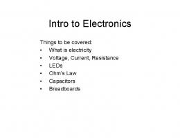
Figure 11: Input for a title page \begin{document} \thispagestyle{empty} \vspace*{\fill} \centerline{\Huge \bf The Ultimate Book} \vspace{1in} \begin{center} by W. Ethan Duckworth\\ Created for his geometry class\\ \today \end{center} \vspace{\fill} \newpage
5.11
Some title pages
Now that we know about commands for fonts, centering, and spacing, we can make some nice title pages. Figure 11 shows you how to combine these commands. The output (on an artificially small page) is in Figure 12. The spacing commands are described in Section 5.8, the centering commands are described in Section 5.7. The command \thispagestyle{empty} tells LATEX not to make any page numbers or headers on this page. The command \today tells LATEX to print today’s date at that spot. The command \newpage forces a newpage to be started at that point.
5.12
Special symbols
Certain symbols have special meaning in LATEX. Some of these are \ $ $$
% ^ _ & # % \{ \}
\ This tells the computer that the following word is a command which should be interpreted. If you want to print \ in text then you should type \textbackslash. If you want to print this in math mode then you should use \backslash. $ This tells the computer to turn on/off math mode (see Section 4.1 for more discussion of this). As a general rule, all math should be done between a pair of $’s, even if the math is so simple that you’re not using fancy commands. Thus, to write 2x = 1 you should use $2x=1$; without the dollar signs you would get 2x=1. Using dollar signs puts the math into a different font which helps the reader tell that they are not reading English anymore. If you want to print $ then you should use \$. % Like any programming language LATEX allows comments. These are statements in the input source, which the computer is not supposed to process, and which don’t show up in the output. For example, if I typed thus $x=\pi$. % because \pi is the area of the circle
thispagestyle today newpage
28
LATEX 2ε guide
W. Ethan Duckworth
Figure 12: Output of a title page
The Ultimate Book by W. Ethan Duckworth Created for his geometry class September 18, 2006
then, the output would just be “thus x = π.” The rest of the words would be for me to see when I was looking at the source input. This is useful if you might forget why you said something, or to help understand a complicated input. If you wanted to print % then you should use \%. ^ and _ In math mode these indicate the presence of a subscript and a superscript. Thus $x_1^2$ produces x21 . If your subscript/superscript is more than one character then you need to enclose it with { and }. Thus $x^23$ produces x2 3 whereas $x^{23}$ produces x23 . To print ˆ and you type \^\ and \_ respectively. & This is used to separate columns in an array (see Section 4.5). To print “&” enter \&. # This is used to represent an argument (input) when defining a new command (or macro). To print “#” enter \#. { and } are used for grouping and defining inputs to LATEX commands, as shown for the exponent x23 above. If I want to print { and } I enter \{ and \}.
5.13 enumerate item
Lists
LATEX has lots of nice facilities for making lists. Let’s start with a simple numbered list. This is created by the enumerate environment. Each new item in the list is created with the \item command. An example of the input and output of a simple list is shown in Figures 13 and 14. You can change the way the numbers look, for example to make your list like like a classical outline. I think that there are packages that do this automatically, but I haven’t bothered looking them up because it’s easy to do manually. At the simplest level you can override the automatic numbering for a specific item. Just type \item[5.] to produce number “5.” . Note, here I had to remember to put the period “.” in. Similarly, if I wanted part (c) I would have to type \item[(c)], not just \item[c].
labelenumi
Now suppose I wanted to have automatic, outline-type numbering. I would re-define the built-in LATEX format which is controlled by the \labelenumi and \labelenumii com-
LATEX 2ε guide
W. Ethan Duckworth
Figure 13: Input for an enumerate list \begin{enumerate} \item This is the first problem. \item This is the second problem. \begin{enumerate} \item This is part (a) of the second problem. Notice that it wraps the words nicely so that the label stands out in the left margin. This behavior was automatic. \item This is part (b) of the second problem. \end{enumerate} \item This is the third problem. \end{enumerate}
Figure 14: Output for an enumerate list 1. This is the first problem. 2. This is the second problem. (a) This is part (a) of the second problem. Notice that it wraps the words nicely so that the label stands out in the left margin. This behavior was automatic. (b) This is part (b) of the second problem. 3. This is the third problem.
29
30
LATEX 2ε guide
W. Ethan Duckworth
Figure 15: Input for an outline-type list \begin{enumerate} \renewcommand{\labelenumi}{\Roman{enumi}.} \renewcommand{\labelenumii}{\Alph{enumii}.} \item This is the first item. \item This is the second item. \begin{enumerate} \item This first sub-item. \item This is the second sub-item. \end{enumerate} \end{enumerate}
Figure 16: Output for an custom outline type list I. This is the first item. II. This is the second item. A. This first sub-item. B. This is the second sub-item.
mands. I’ll use the \renewcommand command which is described in Section 5.15. Figures 15 and 16 show how to do this. itemize
The itemize environment gives you a list without numbers. A sample of this list is given in Figures 17 and 18.
description
The description environment makes a list where you provide the heading for each new list item. An example is given in Figures 19 and 20.
5.14
Environments
LATEX has function commands that take an argument, like \textbf{This}, and it also has environments that come in a \begin and \end pair. Figure 21 shows some of the environments we’ve used so far, along with a brief description.
Figure 17: Input for an itemize list \begin{itemize} \item This is the first item. \item This is the second item. \begin{itemize} \item This first sub-item. \item This is the second sub-item. \end{itemize} \end{itemize}
LATEX 2ε guide
W. Ethan Duckworth
31
Figure 18: Output for an itemize list This is the first item. This is the second item. – This first sub-item. – This is the second sub-item.
Figure 19: Input for a description list \begin{description} \item[Why I made this list.] I made this list to show you the description list environment. Note that \LaTeX\ will still wrap the words and that the wrapped words are indented. \item[Pointless.] \end{description}
This item is pointless.
Figure 20: Output for an description list Why I made this list. I made this list to show you the description list environment. Note that LATEX will still wrap the words and that the wrapped words are indented. Pointless. This item is pointless.
Figure 21: Environments we’ve seen so far \begin{document} ... \end{document} This contains everything that’s in your LATEX document. You can type stuff after \end{document} and it just won’t show up. This can be useful for leaving notes for yourself. \begin{quote} ... \end{quote} This indents the material in the standard way for longer quotes. I have examples on pages 4 and 25. \begin{center} ... \end{center} This starts a new paragraph and centers the material it contains. At the end it again starts a new paragraph. An example is given on page 22. \begin{equation} ... \end{equation} This creates a displayed equation with a numbered label. An example is given on page (8).
32
LATEX 2ε guide
5.15
W. Ethan Duckworth
User commands and environments
You can, and should, define your own commands (or macros). You should generally put these in the preamble (the stuff between \documentclass and \begin{document}). newcommand
\newcommand creates a new command. For example, the following creates a new command called \ethan: \documentclass{article} \newcommand{\ethan}{W. Ethan Duckworth} \begin{document} The solution of Fermat’s last Theorem, by \ethan. (input)
−−−→
The solution of Fermat’s last Theorem, by W. Ethan Duckworth. (output)
Here {\ethan} means that the name of the new command is \ethan. The stuff {W. Ethan Duckworth} is what the command \ethan will produce. A lot of the time it’s useful to have a command which takes inputs, or arguments. Here’s an example which creates a new command \blank which creates an answer blank with length as an input:
blank
\documentclass{article} \newcommand[1]{\blank}{\underline{\hspace{#1}}} \begin{document} This is an answer blank: \blank{1.5in} (input) This is an answer blank:
↓
(output) Here, the “[1]” in the \newcommand line means that the new command will have one input. The “#1” represents that input in the following definition. Finally, the stuff {\underline{\hspace{#1}}} means that \blank will produce an underline which contains an horizontal space, and the length of the space will be given by the input #1. In Section 4.2 I promised to give an example of a new fraction command that always prints in display mode. It should have two inputs, issue the command \displaystyle, and then use the usual fraction command. Here it is: \newcommand{\dfrac}[2]{{\displaystyle \frac{#1}{#2} }} Using this we would have This fraction $\dfrac {1}{2}$ is big. (input)
LATEX 2ε guide
W. Ethan Duckworth
−−−→
This fraction
33
1 is big. 2
(output)
The definition of \dfrac was given with two pairs of nested {’s as opposed to the usual one. This is so \displaystyle will only affect the \frac command which follows, it will not affect anything outside of the inner pair of { and }. Here’s a more complicated example. On page 3 we saw the command called \map. This was created as follows:
\newcommand{\map}[4]{\begin{array}{ccc} #1 & \longrightarrow & #2 \\ #3 & \mapsto & #4 \end{array}} Here the “[4]” means that “\map” will have four arguments. In the definition that follows those arguments are represented by #1, #2, #3, #4. It takes those arguments, and it makes an array with them and puts some arrows between them. Now we can use it The function is $$ \map A B x {x^2} $$ (input)
The function is A −→ B x $→ x2
−→ (output)
If you try to use \newcommand to create a command and the name for your new command has already been used then you will get an error. If you do want to get rid of the old definition you can use the command \renewcommand which works just like \newcommand. There’s examples of its use on pages 19 and 30. You can also define your own environment. Environments have a \begin command and an \end command. They are useful for enclosing something that’s longer than a sentence or so. The main command is \newenvironment. This command is followed by three pairs of { , }’s: the first pair contains the name, the second contains what the \begin part means and the third contains what the \end part means. For example, suppose you defined
\newenvironment{solution}[1] {\noindent\textbf{Solution. } (by #1)\\} {\par \hrule \par} then if you typed \begin{solution}{Ethan} This is my solution. I hope you like it. You’ll be able to tell where the solution ends by the horizontal line. \medskip \end{solution} (input)
renewcommand
newenvironment
34
LATEX 2ε guide
W. Ethan Duckworth
↓ Solution. (by Ethan) This is my solution. I hope you like it. You’ll be able to tell where the solution ends by the horizontal line. (output) In the \newenvironment definition {solution} gives the name to the environment and “[1]” says that the environment will have one argument. The next part {\par\noindent\textbf{Solution. }(by #1)} par
says that when \begin{solution} is executed, LATEX should start a new paragraph (that’s what \par does), then it should print “Solution. ”, but not indent it, LATEX should print “(by #1)” where #1 is replaced by the input, and finally it should start a new line with \\. The next part
hrule
{\par \hrule \par} says that when \end{solution} is typed that LATEX should start a new paragraph, put a horizontal line across the page, and then start another new paragraph. Finally, I mentioned on page 32 that I would show you how to create your own function names for use in mathematics.
DeclareMathOperator
\documentclass{article} \usepackage{amsopn} % AMS Operator Name \DeclareMathOperator{\lcm}{lcm} Here’s an example of its use: So the least common multiple is $$ \lcm(3, 5) = 15 $$
So the least common multiple is −→
lcm(3, 5) = 15
(output) (input) If you want to have limits on your custom operator name, you use the command DeclareMathOperator*.
5.16
Packages
One of the great strengths of LATEX is the number of add-on packages which have been produced. I mentioned the fullpage package on page 19, and I discussed the commands \text in Section 4.3 and the environment bmatrix in Section 4.6, both of which come from the AMS package amsmath. Now I’ll give you a little overview about packages. A package is an external file that you can load into your LATEX document to add commands and other functionality. usepackage
To load a package you use the command \usepackage. For example, in this document I typed something like \documentclass{article} \usepackage{amsmath,amsthm,graphicx,pdfpages}
LATEX 2ε guide
W. Ethan Duckworth
35
\begin{document} ...... In almost all documents I use amsmath, amsthm (see Section 5.17) and amsfonts (which defines nice fonts for things like R, Z, S, etc). In all cases where I import graphics I use the graphicx package (see Section 6.6 for more information on this package). There are packages for almost any technical application: for making Feynman Diagrams, for numbering and annotating the lines of a play, for typesetting ancient greek, for manipulating PostScript, for various kind of mathematical diagrams, for making hyperlinks in a pdf output, for including graphics, for formatting a bibliography, and finally, for formatting a paper in the proprietary house-style for each professional journal. All common packages are already installed on standard LATEX packages (like MikTeX and TeXShop (which in turn is based on teTeX, a standard Unix distribution)). Other packages are easy to obtain. You just go to www.ctan.org, type in the package name, and download the file. The files are all plain text and you just put them somewhere where TEX can find them (TEX will always find things inside the same directory as the file you’re trying to typeset; after it searches here it will look in various standard locations).
5.17
Theorems, definitions, examples, etc
The amsthm package allows you to easily create different environments for making nice theorems, lemmas, definitions, proofs, etc. It creates a command \newtheorem for creating your own theorem-like environments. “Theorem-like” means anything that looks like a paragraph (or more) and should (possibly) have a bold face heading, should (possibly) have numbering and should (possibly) have a font change. For example, you might type
amsthm newtheorem
\documentclass{article} \usepackage{amsthm} \newtheorem{lemma}{Lemma} \newtheorem{cor}{Corollary} \newtheorem{theorem}{Theorem} This would define three environments lemma, cor, and theorem. Each of these environments (as defined here) would get its own counter. For example, if you typed \begin{lemma} Let $x$ and $y$ be even numbers. \end{lemma}
Then $x+y$ is even.
\begin{cor} If $x+y$ is odd then one of $x$ and $y$ is odd. \end{cor} you would produce the document in figure 22. Note that LATEX took care of all the formatting: Lemma was in bold, there was a little extra space above and below the lemma, the font was put into italic mode, the results were numbered, etc. There are three variations on how the numbering works. If you type \newtheorem*{lemma}{Lemma}
numbering
36
LATEX 2ε guide
W. Ethan Duckworth
Figure 22: Example of a lemma and proof Lemma 1. Let x and y be even numbers. Then x + y is even. Corollary 1. If x + y is odd then one of x and y is odd.
then the lemma environment will not be numbered. If you type \newtheorem{lemma}{Lemma}[section] Then the lemmas in Section 5 will be numbered as 5.1, 5.2, etc. and in Section 6 will be numbered as 6.1, 6.2, etc. Now suppose you have defined lemma, with some kind of numbering. If you typed \newtheorem{cor}[lemma]{Corollary} then the corollaries will use the same numbering as the lemmas. Thus you would have something like Lemma 1, Corollary 2, Lemma 3, Lemma 4, Corollary 5, etc. The amsthm package also defines a nice proof environment. If you type \begin{proof} The proof is obvious. \end{proof} you get Proof. The proof is obvious. Traditionally statements of lemmas, corollaries, theorems, etc., are given in italics font; this signals to the reader that the what is written has special status: it is logically true, but that this fact is not obvious, and will require proof. However, definitions and examples do not usually get this treatment, but you still might want them to get similar headings and numbering to lemmas, corollaries, etc. This can be accomplished by using \newtheorem and changing certain style settings. theoremstyle
If you typed \theoremstyle{definition} \newtheorem{example}{Example} you will get something which works just like lemmas, corollaries, etc., but which does not use italics font.
LATEX 2ε guide
6
W. Ethan Duckworth
37
Fancier stuff
6.1
References within document
Automatic reference numbering for things within the document is done with three commands, \label, \ref, \pageref. You use \label to mark something for use later. For example, if you type
label, ref, pageref
\begin{equation} \label{really_important_equation} E = mc^2 \end{equation} this produces
E = mc2
(10)
You use \ref to refer to this equation number, and \pageref to refer to the page the equation occurs on. Thus We see that Equation \ref{really_important_equation} occurs on page \pageref{really_important_equation}. will produce:
“We see that Equation 10 occurs on page 37.”
Note, to get the label and reference system to work correctly, you have to run LATEX twice if there have been any changes in the labels. This is because the result of a label is stored in an auxiliary file (like foo.aux if your text file is foo.tex). When LATEX sees a \ref it reads in the numbers from the aux file; this information was left there from the previous LATEX run. If the numbers haven’t changed since the last run then everything is correct; otherwise, run LATEX again and you’ll get the correct numbers.
6.2
Run twice!
Bibliography and citations
There’s more than one way to do bibliographies; I’ll tell you about a great package called amsrefs. To use this package you would load \usepackage{amsrefs} in the pre-amble. To refer to an item in the bibliography you use \cite. Suppose I typed Two excellent examples are \cite{duckworth1} and \cite{strunk1918} This would produce “Two excellent examples are [1] and [2].”
amsrefs cite
The entries for the bibliography are created later, and are given the keys duckworth1 and strunk1918. Here’s what it would look like: \begin{bibdiv} \begin{biblist} \bib{duckworth1}{report} { author = {Duckworth, W. Ethan}, title = {A Short Course in Galois Theory}, organizaation={Loyola College}, type = {Lecture Notes},
bibliography
38
LATEX 2ε guide
W. Ethan Duckworth
Figure 23: Standard bibliography
References [1] W. Ethan Duckworth, A Short Course in Galois Theory, Lecture Notes, Loyola College, Spring 2005. [2] William Strunk, The Elements of Style, Humphrey Press, Geneva, New York, 1918.
date = {Spring 2005} } \bib{strunk1918}{book} { author = {Strunk, William}, title = {The Elements of Style}, publisher = {Humphrey Press}, address = {Geneva, New York}, date = {1918} } \end{biblist} \end{bibdiv} Note that there is no formatting in how I entered this bibliography, but that the entries are very logical and clear. I didn’t have to worry about how to format dates, or titles; actually, it didn’t even matter what order I put them in. I only had to identify which piece of information was the date, which piece the author etc, and the program took care of everything else! This is so wonderful, you have no idea! Other keys (or keywords, if you like) for pieces of information are journal, volume, number, pages. See the amsrefs documentation for more detail. Figure 23 shows the output from a standard bibliography format. Now, suppose I wanted different types of citations? Well, I can use the exact same code that I entered before, and simply declare some different options when I load the amsrefs package. For example, if I enter \usepackage[alphabetic]{amsrefs} then my bibliography will magically appear as in figure 24. If I enter \usepackage[author-year]{amsrefs} then my bibliography will magically appear as in figure 25.
6.3
Color
It’s easy to tell LATEX to typeset things in color. You load the package color, and then use one of the following two forms of commands: {\color{...}....} For example, if I typed
or \textcolor{...}{....}
LATEX 2ε guide
W. Ethan Duckworth
Figure 24: Bibliography with amsrefs and alphabetic option Loading \usepackage[alphabetic]{amsrefs} and typing Two excellent examples are \cite{duckworth1} and \cite{strunk1918} would produce: “Two excellent examples are [duckworth1] and [strunk1918].”
References [duckworth1] W. Ethan Duckworth, A Short Course in Galois Theory, Lecture Notes, Loyola College, Spring 2005. [strunk1918] William Strunk, The Elements of Style, Humphrey Press, Geneva, New York, 1918.
Figure 25: Bibliography with amsrefs and author-year option Loading \usepackage[author-year]{amsrefs} and typing Two excellent examples are \cite{duckworth1} and \cite{strunk1918} would produce: “Two excellent examples are (Duckworth, Spring 2005) and (Strunk, 1918).”
References Duckworth, W. Ethan. Spring 2005. A Short Course in Galois Theory, Lecture Notes, Loyola College. Strunk, William. 1918. The Elements of Style, Humphrey Press, Geneva, New York.
39
40
LATEX 2ε guide
W. Ethan Duckworth
Figure 26: Output of a blue solotion Example: find the derivative of sin(x). Solution: The derivative is defined as lim
h→0
sin(x + h) − sin(x) h
We use the additive identity for sin(x), etc. So we see that the derivative of sin(x) is cos(x). Example: find the derivative of cos(x).
\documentclass{article} \usepackage{color} \begin{document} This really \textcolor{red}{STANDS OUT} \end{document} I would get This really STANDS OUT I use the declaration mode \color if I want to color everything that is already contained within some other environment or pair of { , }’s. For example, if I wanted to color everything that was in some solution blue, I could use this input: Example: find the derivative of $\sin(x)$. \begin{solution} \color{blue} The derivative is defined as $$ \lim_{h\to 0} \frac{\sin(x+h)-\sin(x)}{h} $$ We use the additive identity for $\sin(x)$, etc. So we see that the derivative of $\sin(x)$ is $\cos(x)$. \end{solution} Example: find the derivative of $\cos(x)$. etc. The output is shown in Figure 26. In this example the point is that \color{blue} will affect all of the stuff between \begin{solution} and \end{solution}. The alternative with \textcolor would be slightly more complicated, I’d have to type \begin{solution} \textcolor{blue} {The derivative is defined as
LATEX 2ε guide
W. Ethan Duckworth
41
Figure 27: Output of a white solution Example: find the derivative of sin(x). Solution: The derivative is defined as lim
h→0
sin(x + h) − sin(x) h
We use the additive identity for sin(x), etc. So we see that the derivative of sin(x) is cos(x). Example: find the derivative of cos(x).
etc. So we see that the derivative of $\sin(x)$ is $\cos(x)$.} \end{solution} Here I had to add a pair of { and } around the material, one an the beginning and one at the end. In any case, of course it’s stupid to color the solution blue. The way I’ve actually used this is to color the solution white. This leaves a blank space that is about the right size for a student to write the solution in (you can make the blank space bigger by adding the declaration \Huge). The output with \color{white} is shown in Figure 27. Certain colors are pre-named in all LATEX formats: black, white, red, green, blue, cyan, magenta, yellow. Thus I can type {\color{red} This is red} and get This is red. I could also type \textcolor{blue}{This is blue} and get This is blue. It is simple to define new colors, and to give them names. If you use LaTeX=>dvi then there are a bunch of names already defined for the dvi driver. Otherwise, you can define your own, or load the names, as described below. For instance, I could type \definecolor{EthanRed}{rgb}{.85,.1,.1} and now I will use it: {\color{EthanRed} This is Ethan Red} (input)
−−−→
and now I will use it: This is Ethan Red (output)
Here the syntax {rgb} names the color model being used: “Red Green Blue”. The three numbers which follow indicate how much red, how much green and how much blue light to use. You can also use {cmyk} which stands for “Cyan Magenta Yellow Black”. If you are going to use a color only once or twice it might not be worth defining a name. In this case, you can specify the color directly as follows: \color[rgb]{1,.1,.1} This is a test \color[cmyk]{.5,.5,1,0} This is a test
This is a test This is a test
42
LATEX 2ε guide
W. Ethan Duckworth
If you want a big namespace of colors pre-defined, you can load the \usepackage[dvipsnames]{xcolor} package. This gives you all the names on the following page.
name
cmyk
color
name
cmyk
GreenYellow
0.15,0,0.69,0
RoyalPurple
0.75,0.90,0,0
Yellow
0,0,1,0
BlueViolet
0.86,0.91,0,0.04
Goldenrod
0,0.10,0.84,0
Periwinkle
0.57,0.55,0,0
Dandelion
0,0.29,0.84,0
CadetBlue
0.62,0.57,0.23,0
Apricot
0,0.32,0.52,0
CornflowerBlue 0.65,0.13,0,0
Peach
0,0.50,0.70,0
MidnightBlue
0.98,0.13,0,0.43
Melon
0,0.46,0.50
NavyBlue
0.94,0.54,0,0
YellowOrange
0,0.42,1,0
RoyalBlue
1,0.50,0,0
Orange
0,0.61,0.87,0
Blue
1,1,0,0
BurntOrange
0,0.51,1,0
Cerulean
0.94,0.11,0,0
Bittersweet
0,0.75,1,0.24
Cyan
1,0,0,0
RedOrange
0,0.77,0.87,0
ProcessBlue
0.96,0,0,0
Mahogany
0,0.85,0.87,0.35
SkyBlue
0.62,0,0.12,0
Maroon
0,0.87,0.68,0.32
Turquoise
0.85,0,0.20,0
BrickRed
0,0.89,0.94,0.28
TealBlue
0.86,0,0.34,0.02
Red
0,1,1,0
Aquamarine
0.82,0,0.30,0
OrangeRed
0,1,0.50,0
BlueGreen
0.85,0,0.33,0
RubineRed
0,1,0.13,0
Emerald
1,0,0.50,0
WildStrawberry 0,0.96,0.39,0
JungleGreen
0.99,0,0.52,0
Salmon
0,0.53,0.38,0
SeaGreen
0.69,0,0.50,0
CarnationPink
0,0.63,0,0
Green
1,0,1,0
Magenta
0,1,0,0
ForestGreen
0.91,0,0.88,0.12
VioletRed
0,0.81,0,0
PineGreen
0.92,0,0.59,0.25
Rhodamine
0,0.82,0,0
LimeGreen
0.50,0,1,0
Mulberry
0.34,0.90,0,0.02
YellowGreen
0.44,0,0.74,0
RedViolet
0.07,0.90,0,0.34
SpringGreen
0.26,0,0.76,0
Fuchsia
0.47,0.91,0,0.08
OliveGreen
0.64,0,0.95,0.40
Lavender
0,0.48,0,0
RawSienna
0,0.72,1,0.45
Thistle
0.12,0.59,0,0
Sepia
0,0.83,1,0.70
Orchid
0.32,0.64,0,0
Brown
0,0.81,1,0.60
DarkOrchid
0.40,0.80,0.20,0
Tan
0.14,0.42,0.56,0
Purple
0.45,0.86,0,0
Gray
0,0,0,0.50
Plum
0.50,1,0,0
Black
0,0,0,1
Violet
0.79,0.88,0,0
White
0,0,0,0
color
44
LATEX 2ε guide
6.4
W. Ethan Duckworth
Conditional commands
Because LATEX is a computer language, you can use conditional statements (as well as loops). I use this to make versions of a quiz within the same document. In other words, Quiz A, Quiz B, and Quiz C, are all stored in the same document, the directions are all the same etc, only some part of the problem changes depending on which version I’m printing. ifx, else, fi
Here’s an example, complete with preamble: \documentclass{article} \let\version C \newcommand{\problem}[3] {\ifx\version A #1 \else \ifx\version B #2 \else #3\fi\fi} \begin{document} \centerline{\Large \bf Quiz 8\version} Find the absolute max and min of the following function: $$\problem {x^3-3x+1 \text{ on }[0,3]} {2x^3-3x^2-12x+1 \text{ on }[-2,3]} {x^3-6x^2+9x+2 \text{ on }[-1,4]} $$ \end{document} Let’s walk through this example carefully.
let
The command \let works just like in other computer languages, it sets the command \version to whatever comes next, in this case “C”. The new command \problem has three arguments. These will be the version A problem, the version B problem and the version C problem. The commands \ifx, \else and \fi go together. This is the syntax for a primitive if-then-else construction. In other words \ifx P Q R S ... \else T U ... \fi means “ if P equals Q then do R, S, . . . otherwise do T, U, . . . ”. Specifically, \ifx stands for “expanded if”: it “expands” the meaning of P and Q, if they are equal then it executes R and S and . . . , otherwise it executes T and U and . . . . The \fi tells LATEX that it has reached the end of the \else statement. Now that you understand \ifx ... \else ... \fi you can see that the definition of problem essentially says, “If it’s version A, then print the first problem, otherwise, if it’s version B then print the second problem, otherwise print the third problem”. If I typeset the above document as it is, I’ll get something like figure 28. If I change the line \let\version C to \let\version A I’ll get something like figure 29.
6.5
Block comments with conditionals
A useful feature of LATEX (and any computer language) is the ability to make comments. These are things you can read when you look at the source code, but don’t show up in the printed output. For example:
LATEX 2ε guide
W. Ethan Duckworth
45
Figure 28: Conditional Quiz version C
Quiz 8C
Find the absolute max and min of the following function: x3 − 6x2 + 9x + 2 on [−1, 4]
Figure 29: Conditional Quiz version A
Quiz 8A
Find the absolute max and min of the following function: x3 − 3x + 1 on [0, 3]
Thus, $x^n + y^n = z^n$ does have a solution % as long as we allow irrational numbers would only show “Thus, xn + y n = z n does have a solution” and the extra comment would be hidden so that you, the author, can see it, but the reader cannot. Using %’s to comment out lines is convenient only for small portions of code. For larger portions it’s nice to have a command that marks the beginning and end of the comment. There is more than one way to do this in LATEX, probably the best is with the verbatim package. So, if you load \usepackage{verbatim} you can then type:
comment
Thus, $x^n + y^n = z^n$ does have a solution \begin{comment} None of the stuff in here will be seen. Imagine that there were a page or two of stuff here. \end{comment} and again, when you typeset this, it would show only: “Thus, xn + y n = z n does have a solution”. Be careful though: the comment environment has the unusual affect of hiding everything that is on the same line as \begin{comment} or \end{comment}. Thus, if you typed \begin{comment} This is hidden. \end{comment} What about this? you would not see “What about this?”. Now, you can combine block comments like this with the ability to define your own environments, to either show all comments or not depending on your mood (or, more usually,
Warning
46
LATEX 2ε guide
W. Ethan Duckworth
Figure 30: Block comment example Fermat’s Last Theorem now follows from the previous work Here are the details. Imagine lot’s of hard stuff here. Here end the details.
depending on whether you’ve forgotten all the details of the proof that you wrote 6 months ago). For example: \documentclass{article} \newenvironemnt{details}{\comment}{\endcomment} \begin{document} Fermat’s Last Theorem now follows from the previous work \begin{details} Imagine lot’s of hard stuff here. \end{details} \end{document} would produce a document that showed only “Fermat’s Last Theorem now follows from the previous work”. If you forgot how the proof went, then you would change your document thus: \documentclass{article} \newenvironemnt{details}{\par Here are the details.\par}{\par Here end the details.\par} \begin{document} Fermat’s Last Theorem now follows from the previous work \begin{details} Imagine lot’s of hard stuff here. \end{details} \end{document} Now this would print out as in figure 30. (See Section 5.15 on page 33 for an explanation of newenvironment and \par.) Of course, people often keep both versions of the details command in their source code, and just comment out one or the other using %’s! In other words, most people would have something like: \newenvironment{details}{\comment}{\endcomment} % \newenvironemnt{details} % {\par Here are the details.\par} % {\par Here end the details.\par}
LATEX 2ε guide
W. Ethan Duckworth
47
or % \newenvironment{details}{\comment}{\endcomment} \newenvironemnt{details} {\par Here are the details.\par} {\par Here end the details.\par} Of course, if you want to be really fancy, then you can combine conditional flags as in Section 6.4 with comments. Then you would have something like \let\showdetails T or \let\showdetails F and an \ifx command to check. Thus:
conditional comments
\let\showdetails T \newenvironment{details} {\ifx \showdetails T \par Here are the details.\par \else \comment\fi} {\ifx \showdetails T \par Here end the details.\par \else \endcomment\fi}
6.6
Importing graphics
LATEX can produce some simple pictures internally, but most of the time graphics are produced in an external program and then imported. The main package for controlling how this importing works is called graphicx. Thus, to use the following commands you would put \usepackage{graphicx} in your pre-amble. Much more information on importing graphics can be found in the documentation for graphicx, and in the useful document Using Imported Graphics in LATEX 2ε available at http://www.ctan.org/tex-archive/info/epslatex/english/epslatex.pdf
graphicx
In this scheme, you create a graphic in some external program, you save this graphic in a file somewhere where LATEX can find it. Usually this means save the graphic file in the same folder as the latex source file. If you are using the standard LATEX output format, dvi, then your graphics file should be in Encapsulated PostScript (eps). If your graphic is not in EPS format, then it’s probably best to convert it to EPS. If you are using pdf-LATEX then your graphics file should be in one of the following: PDF (Portable Document Format by Adobe), PNG (Portable Network Graphics, a replacement for GIF), JPEG (Joint Photography Expert Group). The basic command for importing a graphic is \includegraphics. It has a mandatory argument for the filename. For example, I would type \includegraphics{my_graphic_file} If you’re using the standard LATEX output format, dvi, then the includegraphics command will assume that the filename ends in .eps. Thus, you’re file should be eps format and should be named my_graphic_file.eps. If you’re using pdf-LATEX then the command \includegraphics{my_graphic_file} will look first for my_graphic_file.png, if this file does not exist then it will look for my_graphic_file.jpg, if this file does not exist then it will look for my_graphic_file.pdf . The includegraphics command has many optional arguments which control how how the graphic is displayed. For example, \includegraphics[scale = .5]{my_graphic_file}
includegraphics
48
LATEX 2ε guide
W. Ethan Duckworth
would make the graphic half as big. Another example \includegraphics[width=1in, angle = 90]{my_graphic_file} would shrink the graphic until the width is 1in (it would keep the same ratio between the width and height) and then it would rotate it 90 degrees.
6.7
Floating figures
Because LATEX is not a visual editor, there’s one issue that comes up with placing graphics. LATEX will put the graphic wherever you put the includegraphics command. However, LATEX will also try to decide where to put page breaks, and how to space paragraphs, etc. All of this works perfectly if the graphic is going at the top of page 1, at the end of the last page, or if you know that it will wind up in the middle of a page. But, if the graphic ends up where LATEX would like to put a page break between pages n and n + 1, then LATEX has to decide whether to keep the graphic on page n, and squeeze stuff to make it fit, or put it on page n + 1 and expand stuff to fill some of the empty space.
figure
Anyway, these decisions result in less than optimal spacing. A better solution is to let LATEX float the figure, moving it before or after some of the words, but keeping the spacing perfect. You do this with the \begin{figure} environment. Thus \begin{figure} \includegraphics{my_graphic_file} \end{figure} would create a floating figure, which might be put at the top of this page, or maybe at the top of the next page. If you let LATEX do this, then you won’t know as you type exactly where the graphic will appear. Thus, you would avoid saying things like According to the graph below \includegraphics{my_graphic_file} we see that the limit is 1.
caption
Instead, you would use \label and \ref to refer to the figure. This requires that you create a number for the figure. This is done with \caption. Thus, a complete example would be: According to the graph in figure \ref{really_important_figure} we see that the limit is 1. \begin{figure} \caption{My important graph} \label{really_important_figure} \includegraphics{my_graphic_file} \end{figure} So, do I really do this every time I include a graphic? No. I usually start by just including it where I want. Then, if the spacing looks screwed up, rather than manually moving it around myself, I make it into a floating figure.
LATEX 2ε guide
7
W. Ethan Duckworth
49
Other references
I’ve given you this guide, but I’ve tried to keep it as short as possible, so let me mention some other sources of information. Guide to LaTeX by Helmut Kopka, Patrick W. Daly. This is one of the standard references, and, best of all, it’s in the library! http://www.giss.nasa.gov/latex/ltx-2.html, this is a web-page glossary. This is perfect for a quick look at how to use a command like \frac. Frankly, this may be all you need for now. “Getting started with LATEX”, by David R. Wilkins at http://www.maths.tcd.ie/~dwilkins/LaTeXPrimer/GSWLaTeX.tex. This is about 45 pages and covers most of the things you need to know. Note that this file is the input source, so you can edit it, copy it, see how Wilkins did it etc. You can also view this document in html at http://www.maths.tcd.ie/~dwilkins/LaTeXPrimer/ and get the dvi version of the output (by the way, it’s easy to convert dvi to pdf). “The Not So Short Introduction to LATEX 2ε ”, by Tobias Oetiker, at ftp://cam.ctan.org/tex-archive/info/lshort/english/lshort.pdf This one is about 150 pages, talks about everything, margins, lists, math, special symbols, etc. Since many of you will be using TeXnicCenter, you should learn about what things it can do. In particular, it can insert all kinds of LATEX commands and math constructions. Find out more about it at http://www.texniccenter.org. I’ve also had great luck with specific topics doing a Google search, like “latex change margins” (although with google you often find a weird bunch of sites that specialize in latex rubber products!).
... ··· ...
\dots \cdots \ldots
..
.
.. .
\leftarrow \Leftarrow \longleftarrow \Longleftarrow \rightarrow \to \Rightarrow \Longrightarrow
ι κ λ µ ν ξ π ρ σ
\alpha \beta \gamma \delta \epsilon \varepsilon \zeta \eta \theta \vartheta
α β γ δ % ε ζ η θ ϑ
← ⇐ ←− ⇐= → → ⇒ =⇒
∩ ∪ ∧ ∨ ⊂ ⊆ ⊃ ⊇
+ > < \le \ge \ne \cdot
+ − > < ≤ ≥ $ = · \times \div \ast \circ \otimes \oplus \circ \bullet
\tau \upsilon \phi \varphi \chi \psi \omega \Gamma \Delta
↑ ⇑ ↔ ⇔ ⇐⇒ A→ A−→ :→
\ddots
\vdots
∃ ∀
Θ Λ Ξ Π Σ Υ Φ Ψ Ω
⊥ ∈ 4 ∝ ≈ ∼ = ≡
\Theta \Lambda \Xi \Pi \Sigma \Upsilon \Phi \Psi \Omega
\perp \in \ni \propto \approx \cong \equiv
\exists \forall
D ∠
\triangle \angle
\uparrow \Uparrow \leftrightarrow \Leftrightarrow \Longleftrightarrow \mapsto \longmapsto \hookrightarrow
Some arrows
τ υ φ ϕ χ ψ ω Γ ∆
Greek letters
× ÷ ∗ ◦ ⊗ ⊕ ◦ •
Miscellaneous symbols
\iota \kappa \lambda \mu \nu \xi \pi \rho \sigma
\cap \cup \wedge \vee \subset \subseteq \supset \supseteq
Binary relations and operations
abc
√ n
inf dim ker arg
n
, -* + abcdef
, -* + abcdef
n
abcdef * +, -
abcdef * +, -
\overrbrace{abcdef}^{n}
\overbrace{abcdef}
\underbrace{abcdef}_{n}
\underbrace{abcdef}
\inf \dim \ker \arg
\bigoplus
Some fancy fonts (use \usepackage{amsfonts} ) Name command A, B, C, D, . . . a, b, c, d, . . . Fraktur: \mathfrak A, B, C, D, . . . a, b, c, d, . . . Calligraphic \mathcal A, B, C, D, . . . Black board bold \mathbb A, B, C, D, . . .
Delimiters (resized with \left and \right) symbol command symbol command { and } \{ and \} | | F \| G and H \langle and \rangle
\sqrt[n]{abc}
\sqrt{abc}
\widehat{abc}
) abc abc
\underline{abc}
abc √
\overline{abc}
\lim \log \gcd \sup
Braces and similar constructions
lim log gcd sup
Some trigonometric and similar symbols
\widetilde{abc}
\sin \cos \tan \ln
\bigcup
\bigcap
Variable-size symbols (these take limits) % # ' \sum \int $ & \prod \bigotimes
abc
( abc
sin cos tan ln
"
!
A one page symbol guide for LATEX 2ε (almost all need math mode)
Index $, 27 %, 27 ˆ , 28 , 28 \, 27
\align, 8 \displaystyle, 9 \eqnarray, 8 \equation, 8 \gather, 8 \multline, 8 \documentclass, 6 dollar sign, 27 double spacing, 19
align, 14 amsmath, 10, 12, 13 align, 14 gather, 14 multline, 13 amsrefs bibdiv, 37 biblist, 37 \cite, 37 amsrefs, 37 amsthm, 35 array, 11
\else, 44 \emph, 21, 26 ending paragraphs, 19 ending sentences, 19 \end{document}, 6 environments array, 11 bmatrix, 13 center, 22 comment, 45 description, 30 document, 6 enumerate, 28 figure, 22, 48 itemize, 30 quote, 25 tabular, 11 \everymath, 10
\, 27 \baselinestretch, 19 \begin{document}, 6 \bf, 25 bibdiv, 37 bibliographies, 37 biblist, 37 \bigskip, 23 \blank, 32 bmatrix, 13 build (TeXnicCenter), 6
\fi, 44 figure, 48 caption, 48 figure, 22 \fill, 24, 25 floats, 48 font commands, 25 font sizes, 26 \footnotesize, 26 \frac, 9 fullpage, 19, 34
\caption, 48 \center, 22 \centerline, 22 citations, 37 \cite, 37 color, 38 comments, 27, 45 block comments, 45 conditional comments, 47 conditional comments, 47 conditionals, 44 cross references \label, 37 \pageref, 37 \ref, 37
gather, 14 graphicx, 47 \headheight, 18 \headsep, 18 hello world document, 5 \hfill, 24 \hline, 12 \hrule, 34
DeclareMathOperator, 34 display style, 8 displayed equation, 7 51
52
\hspace, 23 \Huge, 26 \ifx, 44 in-line math, 7 \includegraphics, 47 \int, 9 integrals, 9 \it, 25 \item, 28 itemize, 30 Knuth, Donald, 1, 3, 4 \label, 37 \labelenumi, 28, 30 Lamport, Leslie, 1, 4 \LARGE, 26 \Large, 26 \large, 26 LATEX, 1 \let, 44 \lim, 9 lists description, 30 enumerate, 28 itemize, 30 outline, 30 margins, 18 \medskip, 23 memoir, 19 MikTeX, 5 multline, 13 \newcommand, 32 \newenvironment, 33 \newpage, 27 newtheorem numbering, 35 theoremstyle, 36 \newtheorem, 35 \noindent, 21 \normalsize, 26 packages amsmath, 10, 12, 13 amsrefs, 37 amsthm, 35 color, 38 fullpage, 19, 34 graphicx, 47 memoir, 19 ulem, 26
LATEX 2ε guide
W. Ethan Duckworth
\usepackage, 34 verbatim, 45 \pagref, 37 \par, 34 paragraph ending, 19 paragraph justification, 21 \parindent, 21 \parskip, 21 percent sign, 27 preview, 6 \qquad, 23 \quad, 23 quote, 25 quotion marks, 25 \ref, 37 \renewcommand, 19, 30, 33 \rm, 25 \sc, 25 \scriptsize, 26 sentence ending, 19 \sf, 25 \smallskip, 23 \ , 22 spacing \bigskip, 23 \hspace, 23 \medskip, 23 one space, 22 \qquad, 23 \quad, 23 \smallskip, 23 thin space, 23 \vspace, 23 \sqrt, 8 subscript, 28 \sum, 9 superscript, 28 tabular, 11 TEX, 1 TeXnicCenter, 5 TeXShop, 5 \text, 10 text-editor, 5 \textbf, 25 \textheight, 18 \textit, 25 \textrm, 25 \textsc, 25 \textsf, 25
LATEX 2ε guide
\textt, 25 \theoremstyle, 36 thin space, 23 \thispagestyle, 27 \tiny, 26 title page, 27, 28 \today, 27 \topmargin, 18 \tt, 25 typeset, 6 ulem, 26 usepackage, 19, 34 \vfill, 24 view output, 6 \vspace, 23
W. Ethan Duckworth
53