Introduction to linear programming as a popular tool in optimal ...

Advances in Environmental Biology, 9(3) February 2015, Pages: 906-917

AENSI Journals

Advances in Environmental Biology ISSN-1995-0756

EISSN-1998-1066

Journal home page: http://www.aensiweb.com/AEB/

Introduction to Linear Programming as a Popular Tool in Optimal Reservoir Operation, a Review 1Mohammad

Heydari,

2Faridah

Othman,

3Kourosh

Qaderi,

4Mohammad

Noori and

5Ahmad

ShahiriParsa 1

PhD candidate, Faculty of engineering, University of Malaya, Kuala Lumpur Associated professor, Department of civil Engineering, Faculty of Engineering, Kuala Lumpur, Malaysia Assistant Professor, Department of Water Engineering, Shahid Bahonar University of Kerman, Iran 4 PhD candidate, Faculty of Engineering, Ferdowsi University, Mashhad, Iran 5 Graduated student, Faculty of Engineering, University of UNITEN, Kuala Lumpur, Malaysia 2 3

ARTICLE INFO Article history: Received 21 November 2014 Received in revised form 4 December 2014 Accepted 3 January 2015 Available online 28 January 2015 Keywords: Linear programming, LP, optimal operation, multiple reservoirs, optimization, mathematical modeling.

ABSTRACT Water is a rare and vital natural resource for all biological phenomena and human activities that continuously is needed to be known at any time and place. Taking into the burgeoning growth of population and consequently increasing human needs, the limitation of water resources is a considerable challenge for human. Moreover, asymmetrical distribution of rain time and location in most countries has caused that the water resources management and programming be considered. In order to resolve this problem, researchers are trying to use some techniques in relation with programming and management for a long time. Most of practical and applied problems can be modeled as a linear programming problem regarding all intrinsic complexities. The mentioned reason and also presence of different solving software of linear programming problems have caused that linear programming be used as one of the most practical methods in the field of dam operation for years. In this research, we introduce optimal operation problems of reservoirs by using linear programming techniques and discuss about them. Also, objective and multi objective models were introduced by using some questions. Finally, some popular methods in the field of modeling such problems are introduced.

© 2015 AENSI Publisher All rights reserved. To Cite This Article: Mohammad Heydari, Faridah Othman, Kourosh Qaderi, Mohammad Noori, Ahmad ShahiriParsa. Introduction to linear programming as a popular tool in optimal reservoir operation, a Review. Adv. Environ. Biol., 9(3), 906-917, 2015

INTRODUCTION Water is the most important requires for all living creatures after oxygen. Life and health of all beings containing human, plants and animals, depends on water. Therefore, nowadays, water is known as human treasure. Although 75 percent of planet earth is composed of water, but only one percent of the fresh water is usable. In spite of the fact that the amount of usable water (drinking water) on earth is limited, but this insignificant amount is not spread on the earth uniformly. This limitation is one of the most important and essential challenges in countries with arid and semi-arid regions. On one hand, limited access to water resources and on the other hand, human need for water, necessitate the proper management strategies. Taking into aims like providing water, controlling floods, hydro power production, tourism, etc. dams are designed and constructed in order to resolve such problems. Providing water for municipal, agricultural and industrial consumption is one of the main purposes for reservoir operation and planning. In most countries, agricultural purposes has the highest water level consumption. So, optimal operation and management of water resources, among giving proper response to the needs of this part, leads to reduced waste water and increasing the level of yield of production and gaining sustaining development in agriculture [1]. Flood control and decreasing its resulted damage are another aims of constructing dams. Besides dams as main sources in providing water, these also have high capacity in the field of growing and developing tourism industry. In most countries in the world, dams and their reservoirs are counted as the most important tourist absorption and absorb numerous tourists annually. One of the aims of constructing dams is hydroelectric Corresponding Author: Faridah Othman, Associated professor, Department of civil Engineering, Faculty of Engineering, Kuala Lumpur, Malaysia. Ph: 0379674584; E-mail: [email protected]

907

Mohammad Heydari et al, 2015 Advances in Environmental Biology, 9(3) February 2015, Pages: 906-917

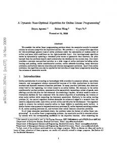
energy. Nowadays, the hydropower and thermal energies have the highest share in producing the world`s electricity. Although, problems and limitations of producing electricity in thermal power sources and due to technical issues, the imperatives of environmental criteria, resources constrains have caused that, by the time the general trend in the world of power generation, hydroelectric plants will be more attentive. The potential energy of water behind a dam, provide hydroelectric energy. In this case the energy of the water depends on stored water of dam and height difference between the water source and the withdrawal of water from the dam. Power generation in hydroelectric plants has a lot of advantages. Perhaps these benefits have caused that this production method has comparative advantages and are considered in the world, especially in countries where water resources are relatively substantial. By constructing the dam in areas of water in the river and the regions where rainfall is high and installing turbine, the gravitational potential energy of water behind the dam can be used to generate hydroelectric power. The next issue is the optimal operation of the reservoir, considering the objectives like drinking water needs, industrial, agricultural, hydroelectric purposes, flood control, tourism and etc. For this purpose, efficient approaches and appropriate solutions must be considered for operating reservoirs as one of the most important components of water resources. Application of such approaches leads to create balance between available limited resources and high consumption, optimization of water use in agriculture, municipal and industry and finally sustainable development in water resources management. Nowadays, the water management and water protection are high importance in developing and developed countries. In order to system enhancement and equitable management of water resources, using the principles and technical planning is necessary. Using planning technique practical and practicable in order to optimize water resources, due to its simplicity and applicability has special status. Charles Revelle in 1969 decided to act for design and reservoir management by linear programming and using a Linear Decision Rule (LDR). In this linear decision making method, reservoir outflow in whole operation period calculated as the difference between the storage of the reservoir at the beginning of the period and decision parameter by solving linear programming [2]. In 1970, Loucks applied the linear model with its probable limitation and its deterministic equivalent for solving the system of reservoirs. Cai and his collaborators in 2001, used genetic algorithm with linear programming in complex problems of water reservoir. The gained results have been reported very satisfactory [3]. in 2005, Reis et al. used combination of Genetic Algorithm (GA) and Linear Programming (LP) method designed and solved planning and decision-making for reservoirs of water systems during the probabilistic [4]. in 2006, Reise and his associates in performed a combination method using genetic algorithm (GA) and linear programming (LP) in order to achieve operational decisions for a system reservoir that is applied during optimization term. This method identifies a part of decision variables named Cost Reducing Factors (CRFs) by Genetic Algorithm (GA) and operational variables by Linear Programming (LP) [5]. Optimization Process: The optimization process of this study is presented in Figure 1, and it consists of seven vital steps. 1) A detailed view 2) Problem definition 3) Developing mathematical model 4) Finding solution for the model 5) Sensitive analysis phase 6) Validation 7) Performing the solution Fig. 1: Schematic representation of optimization process.

908

Mohammad Heydari et al, 2015 Advances in Environmental Biology, 9(3) February 2015, Pages: 906-917

1. The first step in this process is expanding a clear understanding of the problem with a detailed view of the real world. To this end, a number of primitive solutions to achieve objectives must be defined that consider different aspects of the problem. Also, some doubts should be in the minds of decision makers as to which opinion to achieve the goal is best. 2. Problem definition phase is a phase in which a precise and clear statement of the problem taken from observations must be made and be gained in identification phase and transparency step of the problem. The mentioned problem definition should define purpose, the influence of the initial solutions, assumptions, barriers, limitations and possible available information on sources and markers involved in the problem. Experience shows that erroneous definition of the problem leads to analysis failure. 3. When we define the problem, the next step is developing a mathematical model. The mathematical model is mathematical performance of the system or real problem and is able to perform different aspects of the problem in interpretable form. At first it may be that qualitative model structure itself, including unofficial descriptive approach. In this unofficial qualitative model, an official model may develop. (Part 3 contains some applied models in order to optimize reservoir operations of dams.) 4. After formulating and developing the model, it is turn to find a solution for the model. Usually the optimal solution for the model with evaluation outcome sequence is found. This sequence of operation starts from a primitive solution that is as input of the model and the generation of the developed solution as output that is known as repeat is resulted. The developed output is resubmitted as a new input and the process is repeated under the certain circumstances. 5. Another important phase of this study is sensitive analysis phase. Performing the sensitivity analysis allows us to determine the necessary accuracy on input data and understanding the decision variables that have the highest influence on the solution. The sensitivity analysis allows the analyst to see how sensitive the preferred option of changing assumptions and data is. By performing the sensitivity analysis, we will be able to recognize how strong is a preferred opinion and input data what need to change to become an optimal choice. In sensitivity analysis, analyst modifies the suppositions or data to enhance the considered option and convert it into optimal choice. Amount of default modification is measuring is determining the power of the model. 6. A solution should be tested. Often the solution is tested in a short or long term. The proposed solution must be validated against the actual performance observation while the test is being made, and also it should be independent of how an optimal solution is obtained. 7. The final phase is performing the solution. This is the step of using optimal outputs for decision making process. Usually, analyst converts his mathematical findings as a series of understandable and applicable decisions. It may be necessary to train decision-makers to help them apply the findings to attain the required changes from the current situation to the desired situation. Also, they need to be supported until they learn the mechanism of maintenance and upgrading the solution.

Fig. 2: Allocating the capacity of reservoir to different volumes (adopted from [6]).

909

Mohammad Heydari et al, 2015 Advances in Environmental Biology, 9(3) February 2015, Pages: 906-917

Reservoirs Operation Modelling: The main objective of optimization is finding the best acceptable solution. There may be different solutions for a problem that in order to compare them and choose the optimal solution, the objective function is defined. The choice of this function depends on the nature of the problem. An Optimization problem with one objective is called (single objective problems), and When several objectives and criteria are considered for minimizing or maximizing the optimization problem, then it is called (multi-objective optimization problems). Some conditions of optimization model structures for the operation of the reservoir are given in below. Single objective models: Objective function by minimizing the total flood damage in its simplest form is defined as a function of flow rate in vulnerable areas as follows: Min Z = (t Є T) (1) Subject to: f(It,Rt) = 0 (2) Rt ≥ Rmin (3) Rt ≤ Rmax (4) St+1 = St + It - Rt (5) Smin ≤ St+1 ≤ Smax (6) │Rt+1 - Rt│≤ ЄR (7) Where: Z: value of objective function Qt: flow rate at damage point t: time index T: time horizon of operation It: flow rate Rt: reservoir outflow that their relationship is expressed by the function as a power constraint. St: reservoir storage Rmin and Rmax: minimum and maximum release values. ЄR: limiting the maximum difference between release values at two successive time steps It: inflow to the reservoir In other models as seen in the relations 8 to 11, the released volume in studied periods is considered as a function of the river basin or reservoir storage. Among these, the function that estimated best value of the objective function is selected as optimal function. This function performs some constant factors for any period during the statistical term. According to it, the release amount can take a percentage of the river basin, save volume or a combination of both. The following is with agricultural purpose and for a reservoir: Min Def =

2

(8)

Subject to: St+1 =St - Qt - Rt – Lt (St, St+1)- Spt (9) Smin ≤ St ≤ Smax (10) Rmin ≤ Rt ≤ Rmax (11) Where: Def: the monthly shortage Rt: released volume of reservoir Dt: amount of the required monthly Dmax: maximum required during a statistical period St: storage volume at the beginning of month Qt: inflow to river during the period t Lt (St, St+1) is calculations of evaporation losses in period t that creates a set of implicit nonlinear equations. Spt: is overflow from the reservoir during the period. Smax and Smin are in order the maximum and minimum volume of reservoir storage, in order to providing the dead storage of the reservoir and renewable and purposes of flood control volume. Rmin and Rmax are in order the minimum and maximum outflow from the reservoir. If a single-objective optimization problem has multiple optimal solutions, it does not matter which one is selected, as they give the same objective function value.

910

Mohammad Heydari et al, 2015 Advances in Environmental Biology, 9(3) February 2015, Pages: 906-917

Yield Model: Discharge model is a linear optimization model. Discharge refers to the flow of future periods with relatively high credit (or with probability equal to or exceeds above) can be supplied. In this model, the relationship between the two series is creating volumetric balance in storage volume during the year. Inter year relations: Sy+ Qy – YFIRM – α P,Y Yp– Ey – Ry = S y+1 αP,Y= Sy≤ka0 Ey= E0 + [ Sr +∑ ( St + St+1 / 2 ) ᵞ1].E In these formulas the various parameters are as follows: Sy: The storage at the beginning of the period Qy: Annual input YFIRM: Annual primary requires Yp: Annual secondary require Ey: Evaporation Ry: Additional output ka0: Storage volume of out year St: Storage volume at the start of the period E: Amount of annual evaporation E0: The fixed amount of annual evaporation ᵞ1: The relative rate of evaporation of the month

(12) (13) (14) (15)

Extra year relations: St + Qt– YFIRM,t –Ypt – et –Rt = St+1 (16) KD + ka0+ St+Kft≤ K (17) et= ᵞt .E0+ ( St + St+1 ) ᵞt .Et (18) In this relation we have: Qt: Average of monthly period et : Monthly evaporation KD: Dead storage Kft: Flooding control volume Because the critical condition determines the reservoir volume, sometimes the relation 15 can be written as follows. St + βt –et – rt =St+1 (19) In this case the model is called the approximate discharge model: βt: The relative coefficient of flow in the driest month of the year To fit the size of the reservoir, this model depends on value and river discharge. In some projects, due to the large fluctuations in discharge and a mismatch between the needs, the model requires reservoir storage volume greater than the existing one. Advantage of discharge model is in performing the results and the simplicity of application in simulation. Moreover, the simulation results clearly show the deficit and reduce the severity of the shortage. Multi-objective: Multi-objective optimization problems (MOPs) are common. They can be either defined explicitly as separate optimization criteria or formulated as constraints. Formally, this can be defined as follows. Definition of Multi-objective Optimization Problem: A general MOP includes a set of n parameters (decision variables), a set of k objective functions, and a set of m constraints. Objective functions and constraints are functions of the decision variables. The optimization goal is to: Maximize y= f (x) = (f1 (x), f2 (x)… fk (x)) (20) Subject to: e(x) = (e1(x),e2(x),…, em(x)) ≤ 0 (21) Where x = (x1, x2… xn) X (22) y =(y1, y2… yn) Y (23) And x is the decision vector, y is the objective vector, X is denoted as the decision space, and Y is called the objective space. The constraints e (x) ≤ 0 determine the set of feasible solutions.

911

Mohammad Heydari et al, 2015 Advances in Environmental Biology, 9(3) February 2015, Pages: 906-917

Feasible Set: The feasible set X f is defined as the set of decision vectors x that satisfy the constraints e.x: Xf = {x X | e (x) ≤ 0} (24) The image of Xf , i.e., the feasible region in the objective space, is denoted as Yf = f (Xf) = Ux Xf {f(x)}. (25) Without loss of generality, a maximization problem is assumed here. For minimization or mixed maximization/minimization problems the definitions presented in this section are similar. In single-objective optimization, the feasible set is completely (totally) ordered according to the objective function f(x). The structure of a basic model that is the base of many optimization modes of reservoirs’ operation is as follows: Minimize Z= (26) Subject to: St+1=St+it-Rt-Et-Lt (t=1,2,3,…n) (27) Smin≤St≤cap (t=1,2,3,…n) (28) 0≤Rt≤Rmax,t (t=1,2,3,…n) (29) St.Et.Lt.Rt≥0 (t=1,2,3,…n) (30) In which, the variables are defined as follows: Z: objective function Loss: operation cost in month t that is function of output and required storage and volume of the reservoir in month t. Rt: released volume of reservoir Dt: amount of monthly need St: volume of storage reservoir in month t n: length of planning period Smax and Smin are in order the maximum and minimum storage of water in reservoir. Rmax is the maximum outflow from the reservoir during period t. Cap: total volume of water stored in the reservoir. Et: amount of evaporation of the reservoir in month t. Lt: volume of water leaks in the reservoir in month t. It: volume of inflow to the reservoir in month t. In the objective function (26), the total losses during the whole operation period is minimum. In another model [7] we have: Minimize F :

2

Continuity equation in each period is as follows: St+1= St+It- rt Max and Min of release value and storage volume in each period: Stmin ≤ St ≤ Stmax t = 1…, NT rtmin ≤ rt ≤ rtmax t = 1,…, NT

(31) (32) (33) (34)

Dt: water requirements in each period t Rt: release of the reservoir in each period t Dmax: maximum demand during the whole period St: storage in reservoir during period t It: Inflow of the reservoir during period t Stmin: minimum storage of the reservoir Stmax: maximum storage of the reservoir Rtmin: minimum release of water from reservoirs Rtmax: maximum release of water from reservoirs Multi-Reservoir and Multi-Objective: Many real-world problems involve simultaneous optimization of several immensely and often competitive. In such problems, there is no single optimal solution. But, rather there is a set of alternative responses. These solutions are optimal in the wider sense. This means that no other solution in the search space when all objectives are simultaneously considered is better than these solutions. These are known as Pareto-Optimal solution. Traditionally, there are different methods that have been described in material OR and can be used when a multi- objective optimization solution of mathematical programming models is being solved. Most methods formulate a combined objective function, and then repeatedly alternative a model in order to producing a

912

Mohammad Heydari et al, 2015 Advances in Environmental Biology, 9(3) February 2015, Pages: 906-917

number of solution. Such methods contain Weighted Objective Function method [8]; ɛ-constraint method [9], combination method, Geoffrin method [8], Sequential Proxy Optimization Technique [10], Tchebycheff method [11], Stepwise method, using the reference point, satisfactory of trade method, search light method and the reference method. The weighting method is very simple and a simple linear combination of objectives, with different weights, produces the trade-off. In the ɛ-constraint method, one of the objective functions are selected in order to optimization and all remained objective functions are converted to constraint by setting the upper limit of each turn. Combination method combines the weighting and the ɛ-constraint method. Other related details can be found in [12, 13].

f1

f1

is dominated

Pareto-optimal front indifferent

Feasible region dominates

f2

f2

Fig. 3: Illustrative example of Pareto optimality in objective space (left) and the possible relations of solutions in objective space (right). Due to the limitation of power from hydroelectric plants, the objective function can be written as : [14] MAX F = In which, F : revenue from reservoirs : The total production of hydropower in reservoir (i) and during period t : The value of hydropower production in reservoir (i) and during periods t. Water balance equation: Vi,t= Vi,t-1 +(Ii,t – Qi,t –EPi,t ).∆t Reservoir water level: ZLi,t≤Zi,t≤ZUi Required water in the lower limit: QLi,t≤ Qi,t≤ QUi,t Electricity production constraints: PLi,t ≤ n i,t ≤PUi,t The boundary conditions: Zi,t =Zi,b Zi,t+1 = Zi,e

(35)

(36) (37) (38) (39) (40) (41)

Where, Vi,t: storage of reservoir (i) in period t Ii,t : inflow of reservoir (i) in period t Qi,t: Outflow average of reservoir (i) in period t EPi,t: Total evaporation and seepage of reservoir (i) in period t Zi,t: The water level of reservoir (i) in period t ZLi,t: The minimum water level of reservoir (i) in period t ZUi,t: The maximum water level of reservoir (i) in period t QLi,t:The minimum discharge capacity of the reservoir (i) to the downstream environmental requirements in period (t). QUi,t: The maximum discharge capacity of the reservoir (i) in period (t) that limits downstream flooding. Ni,t: The output power of reservoir (i) in period t NXi,t:The installed capacity of reservoir (i) PLi,t: Firm capacity of reservoir i in period t PUi,t: The maximum capacity of the power of reservoir (i) in period t

913

Mohammad Heydari et al, 2015 Advances in Environmental Biology, 9(3) February 2015, Pages: 906-917

Zi,1:The water level of reservoir (i) in first period Zi,b: Reservoir water level at the start Zi,t+1: The water level of reservoir (i) in (t+1)th period Zi,e: The water level of reservoir (i) at the end Linear Programming: Classical optimization models are linear, nonlinear and dynamic model. Optimization problems are often divided into linear and nonlinear models. This division is due to the variable relations. It means that if the relation among all variable be linear, then the problem is called linear, otherwise it is called nonlinear. Due to the simplicity of linear programming structure, and applicability of these models as a primitive appropriate model in water resources management systems, possibility of solving problem with large number of variables, no need for assumptions and primary values, researchers tend to use this kind of programming in their researches. Another advantage of mathematical programming is being different solutions (like simplex method, interior point method), the possibility of converting nonlinear problem with linear one, possibility of instant calculation of the final optimal solution. Maximize c1x1+c2x2+…+cnxn Subject to x1, x2,…, xn≥0 a11x1+a12x2+… +a1nxn≤b1 a21x1+a22x2+… +a2nxn≤b2 … am1x1+am2x2+…+amnxn≤bm

(42) (43) (44) (45) (46)

Note that when the objective function represents cost or contained pollutant amount, for example, smaller objective values represent better choices. In such cases, the objective function is minimized. In the above formulation, we assume maximization, as minimization problems can be rewritten into maximization problems by multiplying the objective function by –1. Methods for solving linear programming problems: Essentially, there are two popular methods for a LP model. These models are Simplex method and its variants and Interior point method [15]. These two methods describe practicable solution term, which can be defined as a confined space with constraints and variable bounds. Then the optimal point (best method for solution) of the solution space is found. Main objective of the graphical method is showing acceptable solutions and research limitations. The method has practical value in solving small problems with two decision variables and only few constrains [16]. Simplex is an algebraic method. The flowchart in figure 1 demonstrates the solution steps in short. The basic concepts are geometric that provides a strong intuitive feel for how it works and what makes it different way. Details of the simplex can be found in operations research concepts and cases [17]. The interior point method is particularly efficient for solving large- scale problems. For small LP models, the interior point algorithm requires a relatively wide computing, then after repetition may only an approximation of the optimal solution be obtained. In contrast, the simplex method requires only a few instant repetitions to find optimal solution. For large LP models, the interior point method is very efficient, but it provides only one approximate solution. The comparison between these two methods have been discussed thoroughly in a study by Illés, T. and T. Terlaky [18]. Often, to solve a big-scale linear programming problems, we face specifically structured coefficient matrix. The most common structure is similar to the following matrix: [19]

(47) Where Ai,j are given matrix, by using simplex method in such cases, we are able to maintain a certain structure of each Simplex step.

914

Mohammad Heydari et al, 2015 Advances in Environmental Biology, 9(3) February 2015, Pages: 906-917

Another specific method to solve these types of problems is the decomposition technique, where the optimal solution of Big-scale problems can be formulated by using the sequences of solution in much smaller size. The most popular decomposition method is Dantzig–Wolf method. The discussion of this method can be found in almost every conceptual optimization texts [19]. If the objective function and one or more constraints are nonlinear, then the problem becomes one of nonlinear programming. In the case of only two variables, they can be solved by the graphical approach; however, the feasible decision space may not have vertices, and even if it does the optimal solution might not be a vertex. In such cases, the curves of the objective function with different values have to be compared. This procedure is shown next.

Fig. 4: Steps to solve linear programming problems by using the simplex method. Introducing popular optimization models:

915

Mohammad Heydari et al, 2015 Advances in Environmental Biology, 9(3) February 2015, Pages: 906-917

Nowadays, many optimization models of operational research, including linear model, nonlinear model and integer model can be easily analyzed by using computer software. Among them, some software like GAMS ، GINO ،LINDO ،LINGO ،QSB and TORA can be mentioned. There are many commercial software packages in the market to solve the mathematical models. The solving software package is generally a solver engine, which contains one or more algorithms for solving a specific class or a number of different levels of mathematical models, like simplex and interior point algorithm for solving LP model. Below is a brief introduction to some of the most popular models. Excel Solver: Excel solver is a powerful tool for optimization. This solver can solve most of optimization problems like linear, nonlinear and integer programming. This tool was first created by Frontline Systems, Inc [20]. Excel solver uses Generalized Reduced Gradient (GRG2) algorithm in order to optimizing nonlinear problems and also uses simplex algorithm for solving linear programming [21, 22]. LINDO: LINDO performs a robust solution for linear, nonlinear (convex and non -convex), quadratic, limited degree and integer optimization of probabilities. Demo version can solve models with 300 variables and 150 constrains (including 30 integer numbers) [23]. LINGO: LINGO is considered as a simple and also robust tool for solving linear and nonlinear programming [24]. One of the major advantages of this tool is formulizing big problems briefly and analyzes problems. LINDO and LINGO software were designed by LINDO Systems, Inc. company in order to solving optimization problems in university, industry and business. The mentioned products come with books operation research: applications and algorithms (1994) [25] and an introduction to mathematical programming: applications and algorithms (2003) written by professor Winston [26]. After GAMS, LINGO is the most robust software of operation research. Among the advantages of LINGO in comparison with LINDO or GAMS is its power in order to modeling are problems that are modeled by LINDO, without the need to specify the type of model by the user. While, LINDO and GAMS don`t have such capability. Another important capability of LINGO is having a very robust, simple and complete Help. LINGO is a comprehensive language in order to facilitating all optimization models. Another specification of this software is having different mathematical functions, statistical and probability, ability to read data from files and other worksheets and high ability in analyzing model. GAMS: General Algebraic Modeling System (GAMS) model is professional software in solving mathematical optimization problems [27]. This software has a program for modeling with high capability in order to obtaining optimal value of variables in purpose function of a programming problem. GAMS is used for solving problems like linear programming (LP), nonlinear programming (NLP) and multiple integer programming (MIP) and multiple integer linear programming (MINLP) etc. One important specification of GAMS is that writing its model independent from the solution. Therefore, we can solve the model with different methods (linear, nonlinear and integer) by only making changes in SOLVER. Interpreting the model from mathematical language to GAMS language is often transparent because GAMS use common English words. MATLAB: MATLAB programming is doubtless one of the most robust computing programs in the field of mathematics, engineering and technology. There are many methods for solving linear programming problems. Among them, the simplex method has specific importance and efficiency for solving problems with average size. There are also some ways for solving large problems (equations with many variables). All the mentioned methods are in optimization tool box of MATLAB and these features are used in solving linear programming problems. We can simply write the specific functions and programs by using codes and functions of MATLAB. In the number is high, we can make a toolbox with them by assigning a subtype. In fact, MATLAB is a simple programming language with very developed characteristics. Also, his software is easier than the other computer languages [28]. MPL: (Mathematical programming language), a product of Maximal Software company, is a modeling system that allows developers to model efficient optimization formulation. MPL is able to solve problems with millions of variables and constrains. MPL works with optimization engines like CPLEX and XPRESS and many other robust industrial solvers. Trial versions are just used up to 300 constrains for a limited time. Win QSB: (Quantitative Systems for Business) is a Windows-based decision-making tool. Win QSB is an educational tool includes a number of modules that almost covers all basic methods of operation research and management science. The size of optimization problems can work with Win QSB is almost similar to LINGO and Solver or any other trial version. The model is flexible in almost any field and can analyze all models and parameters. The control chart of this software, in addition to charting, gives users other tools such as Pareto analysis charts,

916

Mohammad Heydari et al, 2015 Advances in Environmental Biology, 9(3) February 2015, Pages: 906-917

histograms, graph and efficiency of the process, analysis of data distribution and the corresponding computations. Discussion and conclusions: Recognizing the problem, formulating the institutional problem, development of the test modeling, selecting optimal solutions, solution analysis, and performing better solution are logical steps to solve optimization problems. So, it has been suggested that the stages of identification and formulation of the problem are vital for successful analysis and performing the problem. Another important issue is the choice of the modeling technique and a special care should be taken from it in optimizing problems. Modeling the optimal utilization system in the reservoirs is of important factors that should be considered. We can mention the followings: 1. Models should be as simple as to be described by terms and also be understandable by non-specialists, those who have no scientific background. 2. If the model is developed in the real world, should be adaptable enough to be able to unify the rapid changes that may be experienced in the current or future world. 3. The model should include all aspects of the problem, not only some details of it. 4. Models should as possible be user friendly. In a mathematical model, the above mentioned features will be like decision variables which define optimal values of the model. The model is selected by decision makers among all known values for a possible solution of the problem. Variables that are not under control of decision maker are performed as random variables or parameters and constant factors. ACKNOWLEDGEMENT The authors would like to acknowledge the University Malaya Research Grant (UMRG) and the Malaysian International Scholarship (MIS) by the Ministry of Education (MOE, Malaysia) for their support. We are most grateful and would like to thank the reviewers for their valuable suggestions that have led to substantial improvements to the article. REFERENCES [1]

[2] [3]

[4] [5] [6]

[7] [8] [9]

[10] [11] [12] [13]

Heydari, M., F. Othman, and K. Qaderi, Developing Optimal Reservoir Operation for Multiple and Multipurpose Reservoirs Using Mathematical Programming. Mathematical Problems in Engineering, 2015. Revelle, C., E. Joeres, and W. Kirby, The linear decision rule in reservoir management and design: 1, development of the stochastic model. Water Resources Research, 1969. 5(4): p. 767-777. Cai, X., D.C. McKinney, and L.S. Lasdon, Solving nonlinear water management models using a combined genetic algorithm and linear programming approach. Advances in Water Resources, 2001. 24(6): p. 667676. Reis, L., et al., Multi-reservoir operation planning using hybrid genetic algorithm and linear programming (GA-LP): An alternative stochastic approach. Water resources management, 2005. 19(6): p. 831-848. Reis, L., et al., Water supply reservoir operation by combined genetic algorithm–linear programming (GALP) approach. Water resources management, 2006. 20(2): p. 227-255. Othman, F., et al. PRELIMINARY REVIEW OF THE OPTIMAL OPERATION OF RESERVOIR SYSTEMS USING OPTIMIZATION AND SIMULATION METHODS. in International Conference On Water Resources “Sharing Knowledge Of Issues In Water Resources Management To Face The Future” 2012. Langkawi, Malaysia. Afshar, M. and R. Moeini, Partially and fully constrained ant algorithms for the optimal solution of large scale reservoir operation problems. Water resources management, 2008. 22(12): p. 1835-1857. Geoffrion, A.M., Proper efficiency and the theory of vector maximization. Journal of Mathematical Analysis and Applications, 1968. 22(3): p. 618-630. Haimes, Y.Y., L. Ladson, and D.A. Wismer, Bicriterion formulation of problems of integrated system identification and system optimization. 1971, IEEE-INST ELECTRICAL ELECTRONICS ENGINEERS INC 345 E 47TH ST, NEW YORK, NY 10017-2394. p. 296-&. Sakawa, M., Interactive multiobjective decision making by the sequential proxy optimization technique: SPOT. European Journal of Operational Research, 1982. 9(4): p. 386-396. Steuer, R.E. and E.-U. Choo, An interactive weighted Tchebycheff procedure for multiple objective programming. Mathematical programming, 1983. 26(3): p. 326-344. Deb, K., Multi-objective optimization, in Search methodologies. 2014, Springer. p. 403-449. Coello Coello, C.A., Evolutionary multi-objective optimization: a historical view of the field. Computational Intelligence Magazine, IEEE, 2006. 1(1): p. 28-36.

917

Mohammad Heydari et al, 2015 Advances in Environmental Biology, 9(3) February 2015, Pages: 906-917

[14] Guo, S., et al., Joint operation of the multi-reservoir system of the Three Gorges and the Qingjiang cascade reservoirs. Energies, 2011. 4(7): p. 1036-1050. [15] Robere, R., Interior Point Methods and Linear Programming. 2012. [16] Turban, E. and J. Meredith, Fundamental of management science, 1994. Irwin/McGraw-Hill, New York. [17] Hillier, F. and G. Lieberman, Operations research concepts and cases. 2005, Tata McGraw-Hill, New Delhi. [18] Illés, T. and T. Terlaky, Pivot versus interior point methods: Pros and cons. European Journal of Operational Research, 2002. 140(2): p. 170-190. [19] Karamouz, M., F. Szidarovszky, and B. Zahraie, Water resources systems analysis. Vol. 38. 2003: Lewis publishers Boca Raton, FL. [20] Fylstra, D., et al., Design and use of the Microsoft Excel Solver. Interfaces, 1998. 28(5): p. 29-55. [21] Del Castillo, E., D.C. Montgomery, and D.R. McCarville, Modified desirability functions for multiple response optimization. Journal of quality technology, 1996. 28: p. 337-345. [22] Kemmer, G. and S. Keller, Nonlinear least-squares data fitting in Excel spreadsheets. Nature protocols, 2010. 5(2): p. 267-281. [23] LINDO Systems, I., What’s Best!Version 12.0,User’s Manual,Taking your spreadsheet beyond “What If?”. 2013, 1415 North Dayton Street Chicago, Illinois 60642, USA: LINDO Systems, Inc. [24] Xie, J.X. and Y. Xue, Optimization modeling and LINDO/LINGO software. Beijing: The press of Tsinghua University, 2005. [25] Winston, W.L. and J.B. Goldberg, Operations research: applications and algorithms. 1994. [26] Winston, W.L., M. Venkataramanan, and J.B. Goldberg, Introduction to mathematical programming. Vol. 1. 2003: Thomson/Brooks/Cole. [27] Brooke, A., et al., A user’s guide, GAMS software. GAMS Development corporation, 1998. [28] Venkataraman, P., Applied optimization with MATLAB programming. 2009: John Wiley & Sons.