3e Conférence Francophone de Modélisation et Simulation "Conception, Analyse et Gestion des Systèmes Industriels" MOSIM'01 - du 25 au 27 avril 2001 - Troyes (France)
SEQUENCING HYBRID TWO-STAGE FLOWSHOP WITH DEDICATED MACHINES F. RIANE, A. ARTIBA
S.E. ELMAGHRABY
Centre de Recherche et d'Etudes en Gestion Industrielle, FUCaM, Mons, Belgium
[email protected] [email protected]
Graduate Program in Operations Research and the Department of Industrial Engineering North Carolina State University, Raleigh NC, USA
[email protected]
ABSTRACT: We treat the n-job, two-stage hybrid flowshop problem with one machine in the first stage and two different machines in parallel in the second stage. The objective is to minimize the makespan. We demonstrate that the problem is NP-complete. We formulate a dynamic program, which is beyond our grasp for problems of more than 15 jobs. We have conducted experimentation to evaluate the time performance the dynamic programming procedure for "small size" problems. KEY WORDS: Sequencing, Hybrid Flowshops, Mixed Linear Programming, Dynamic Programming, Greedy algorithms, Heuristics.
S tag e # 1
1
INTRODUCTION
S tag e # 2
Machine 2
We consider the problem of scheduling n immediately available jobs in a flowshop composed of two stages. All the jobs are initially processed at the first stage which consists of one machine. Then the jobs are transferred to the second stage which is composed of two machines that are dedicated to two different classes of products in the sense that the set of jobs is partitioned into two subsets and each subset goes to only one of these two dedicated machines. Because of the dedicated nature of the machines in stage two we can partition the set of all jobs, denoted by N with n1 =| N | , into two subsets N 2 and N 3 to denote, respectively, the jobs processed on machines 2 and 3 in stage two. We have n m =| N m | for m = 1,2,3 , with N = N1 and n = n1 = n 2 + n3 . No job preemption is allowed, and the jobs can wait between the two stages (unlimited buffer capacity between the two stages of production). The objective is to minimize the makespan. This production process is schematically described in Figure 1. The presence of more than one machine in the second stage gives rise to the "hybrid flowshop" designation of the production facility, which may be identified as n / 2, m(1) = 1, m(2) = 2, R, F // C max . Recall that this notation indicates, respectively, (number of jobs, n)/(number of stages in series, 2), (number of machines in stage 1, m(1) = 1), (number of machines in stage 2, m(2) = 2), (unrelated machines, R), (flowshop, F)/(no restriction)/ (the objective is to minimize the makespan, Cmax ).
Machine 1
Machine 3
Figure 1. Schematic of the production process. Hybrid flowshops are frequently encountered in practice: in the fibers industry [Salvador, 1973]; in flexible manufacturing systems where each production stage might be either a flexible machine or a flexible manufacturing cell [Wittrock, 1988]; in semiconductor manufacturing [Herrmann and Lee, 1992]; in the glass container industry and glass manufacturing industry [Mei, 1996 ; Paul,1979] in the cable manufacturing industry [Narasimhan and Panwalkar, 1984]; in the textile industry and in the furniture industry (where we have encountered it and was the motivation for this study). In addition to its applicability to many industries, the hybrid flowshop structure may also be encountered in several applications in computer systems. Shen & Chen [1972] and Buten & Shen [1973] consider scheduling problems for computer systems with two classes of processors to support a variety of on-line services, in addition to carrying an ever increasing computer load. In section 2 we demonstrate that this problem is NPcomplete, and therefore we must, eventually, resort to
- 591 -
MOSIM'01 - du 25 au 27 avril 2001 - Troyes (France)
heuristics to solve large scale problems. Section 3 briefly discusses the mixed linear program (MILP) representation of this problem, and presents a dynamic program (DP). Section 4 considers four polynomially solvable cases. The evaluation of the computing time performance of these procedures is presented in section 5, and the conclusions are presented in section 6.
machine 2 in the second stage. Note that the total mb ² processing time of the jobs y k is on machine 1 2 and mb ² on machine 2. b ² b² one job w ∈ N 3 has processing times ( ,0, ) . 2 2
2
We claim that this instance of the problem can be
NP-COMPLETENESS
We shall prove the NP-completeness of the problem by reduction from 3-Partition problem, which is a known strong NP-complete problem [Garey et al., 1976]. First, we define for the benefit of the reader, the 3-Partition problem. Instance: Given a finite set A of non-negative integers a k , k = 1,..,3m and a positive integer bound b, with 3m
∑ a k = mb k =1
;
b
c or t > c 2 3 3 2 Consequently, we have the state of the DP model is defined by
A Mixed Integer Linear Program (MILP)
It is possible to construct a mixed integer linear program (MILP) model of the problem rather straightforwardly [Riane et al., 1997b]. It experiences quadratic growth in the number of binary variables which represent the noninterference constraints between pairs of jobs. In the preliminary experiments we have conducted it consumed more time (on commercially available software such as OMP) than the DP model described below, and its relaxation (to regular LP) yielded lower bounds that were inferior to the bounds secured by the other procedures described in [Riane et al., 1997a]. Consequently we concluded that the model remains of - 593 -
(S r , l (S r ), C 2 (σ (S r )), C3 (σ (S r )) ) with
(C 2 (σ ( S r ), C 3 (σ (S r ))∈ Ω(S r ) and
(1) where
l ( S r ) is a generic designation of the last job processed on machine 1 in the subset
Sr .
In the DP model, the decision at stage r and state (S r , l (S r ), C 2 (σ (S r )), C 3 (σ (S r )) ) is to determine
l ( S r ) , the last job in the set. This decision must be done among the r different possibilities.
MOSIM'01 - du 25 au 27 avril 2001 - Troyes (France)
3.2.2 Mathematical formulation Suppose that Ω( S r −1 ) ⊆ Π ( S r −1 ) , which is constructed n! for all the subsets S r −1 . We shall (r − 1)!(n − r + 1)! consider at stage r and subset S r , the r different decisions by the identification of the last job l ( S r ) processed on machine 1. For a particular last job l ( S r ) = j u we know whether ju ∈ N 2 or ju ∈ N 3 . The state transformation function is
(S r , l (S r ), C 2 (σ (S r )), C3 (σ (S r ))) → (S r −1 , l (S r −1 ), C 2 (σ (S r −1 )), C3 (σ (S r −1 )) ) where, for the sake of brevity in notation, we write S r −1 for S r − { j u } . The stage return is the makespan resulting from the decision made at a particular state. We wish to determine the set Ω( S r ) . Consider the subset S r −1 that is augmented by job j u as the last job processed on machine 1, written as ( S r −1 o ju ) to denote the concatenation of j u with S r −1 . Suppose that ju ∈ N 2 .
For each state ( S r−1 , l , C 2 , C3 ) in Ω( S r −1 ) , we compute the two quantities: T2 ( S r −1 , l , C 2 , C 3 | j u ) = max{
∑ p(1, i) + p(1, ju ), C 2 } + p(2, ju )
(3) (4)
i∈S r −1
T3 ( S r −1 , l , C 2 , C 3 | j u ) = C 3 Tm ( S r −1 , l , C 2 , C 3 | j u ) is the temporary completion time on machine m, m = 2, 3 , of subset S r
where
when the last job processed on machine 1 is job j u (there may be more than one). The ‘temporary’ designation shall be changed to ‘permanent’ after dominance considerations. Note that a similar argument applies to the case ju ∈ N 3 This analysis would result in the following set of pairs of completion times: Σ( S r ) = {(T2 ( S r −1 , l , C 2 , C3 | ju ), T3 ( S r −1 , l , C2 , C3 | ju )); ( S r −1 , l , C 2 , C3 ) ∈ Ω( S r −1 ), S r −1 = S r − { ju }, ju ∈ S r }
The set Σ( S r ) thus generated is pruned by dominance. Ω( S r ) ⊆ Σ( S r ) is the undominated set. At this point the Tm ( S r −1 , l , C 2 , C3 | ju ) ’s are given the permanent labels C m ( S r ) ’s, m = 2,3 .
- 594 -
* Denote the optimal makespan for S r by C max (S r ) . It is given by * C max (S r ) =
min
(C2 (σ ( S r )),C3 (σ ( S r )))
max{C 2 (σ ( S r )), C 3 (σ ( S r ))}
The proof of optimality is embedded in the Principle of optimality of DP: there is no question that for each subset S r of jobs, some job must be last on machine 1. We are now left with the subset S r −1 which we know how to schedule optimally. The enumeration of all possible last jobs on machine 1 (job ju in the previous terminology) gives the desired optimum for the subset. Iterating for r = 1,2,..., n should yield the global optimum. 3.2.3
The Computing Complexity of the DP Model There are n stages corresponding to the cardinality of the subsets. In DP stage 1 there is one state and no n decision. In DP stage 2 (there are possible states 2 in this stage) there may be 2 possible decisions at any state (if both jobs are on the same machine in stage 2) corresponding to the two possible terminal jobs. In DP n stage 3 (there are possible states in this stage) 3 there are at most 3 possible decisions at any state (again if all jobs are on the same machine in stage 2). n In general, in DP stage r (there are possible r states) there are at most r decisions (and correspondingly r different sequences). We must evaluate all possible combinations of the pair
C 2 (σ ( S r )) and C 3 (σ ( S r )) . If M max ( S r ) is an upper bound on these values at stage r then the order of the procedure complexity is n n! 2 O M max r . A gross bound on this r! (n − r )! r =1
∑
number may be obtained as follows. Let
M max
denote a upper bound on the makespan of all jobs. Then the DP approach is of time complexity
(
)
2 O M max n 2 n −1 . This actually refers to the number of alternatives investigated rather than the computing complexity since each alternative evaluation may 2 require a time complexity of O( M max n) . Fortunately, the number of different states at each stage collapses quickly due to dominance, and one may normally deal with no more than different sequences at any state. Therefore, empirically speaking, the DP procedure is
(
)
O kn 2 n −1 .
MOSIM'01 - du 25 au 27 avril 2001 - Troyes (France)
4
POLYNOMIALLY SOLVABLE CASES
Although the general problem has been shown to be NP-hard, there are four special cases which can be solved in polynomial time. But before discussing these cases we need to introduce the following notations: Let C max ( H ) denote the makespan of the schedule resulting from heuristic H and
* C max denote the optimal
J ( N m ) denote C max
makespan. Let the makespan of the schedule obtained by applying Johnson’s algorithm to jobs that are routed on machine m, m = 2, 3 in stage 2. In addition, the following notation will be used in the remainder
P21 =
:
∑
p (1, i ) ,
P31 =
i∈N 2
P1 = P21 + P31 , P22 =
∑ p(2, i) ,
i∈N 2 2 Pmax
= max( P22 ; P32 ) .
∑
p (1, i ) ,
i∈N 3
P32 =
∑ p(3, i)
and
i∈N 3
The four polynomially solvable
cases are: Case 1
min ( p (1, i ) ) ≥ max max ( p (m, i ) ) i∈N
m= 2,3 i∈N m
no job waiting time neither on machine 2 nor machine 3 since these two machines are less loaded than machine 1 and thus are always available for processing jobs immediately after their completion on machine 1. This * means that C max =
min ( p (m, i ) ) . ∑ p(1, i) + mmin = 2,3 i∈N
i∈N
m
Considering this result, an optimal sequence consist on placing last in the sequence the job with the minimum processing time in the second stage. The rest of the sequence can be arbitrary. Thus the complexity of this problem is O(n) . Case 2
min min ( p (m, i ) ) ≥ 2 × max ( p (1, i ) )
m=2,3 i∈N m
i∈N
In this case there will be no idle time on neither machine 2 nor machine 3 once they start processing jobs. Then an optimal schedule is obtained by sequencing jobs on machine 1 so that two jobs with the shortest processing times on this machine will be first in the schedule. The optimal makespan is given by:
* Cmax
max min p(1, i ) + ( P22 ; min p(1, i ) + P23 ) ; i∈N 3 i∈N 2 = min 2 3 + + + max min p ( 1 , i ) ( min p ( 1 , i ) P ; P ) 2 2 i∈N 2 i∈N3
Thus, the computational complexity of this problem is O(n) . Case 3
with jobs in
J J C max ( N 2 ) ≥ C max ( N 3 ) + P21
N 2 . It is easy to check that
* J = C max ( N 2 ) . Hence the computational C max complexity of this problem is O(n log n) .
Case 4
J J C max ( N 3 ) ≥ C max ( N 2 ) + P31
This is similar to the previous case with N 3 replacing N2 . One should note that the conditions for these special cases are not only very restrictive, but also are rarely realized in real life problems. 5
m= 2,3 i∈N m
If min ( p (1, i ) ) ≥ max max ( p (m, i ) ) , then there will be i∈N
In this case, the work load on machine 1 and 2 following the Johnson sequence for N 2 dominates the work load of machine 3 also following the Johnson sequence for N 3 even when the latter is processed after the former on machine 1. Then an optimal sequence is obtained by the concatenation of the two Johnson subsequences σ ( N 2 ) and σ ( N 3 ) starting
COMPUTATIONAL EXPERIENCE
All computational experiments were conducted on a micro computer Pentium. The optimum can be (relatively) easily secured (via either MLP1 or DP) when n ≤ 14 . Therefore, to evaluate the performance of the proposed heuristics we considered examples of problems with up to 14 jobs, with processing times that are randomly selected from a normal distribution with means µ1 = 20, µ 2 = 30, µ3 = 40 and variance σ ² = 25 for all machines. The data for the jobs is given in Table 1., and the results are summarized in Table 2. In Table 2 an entry of 0 time means that it is less than 1 second. Note that the sharp increase in the computing time under DP and MILP as the number of jobs exceeds 10. The MILP relaxation (to regular LP) yields lower bounds that are inferior to the one secured by LB procedure of described in [Riane et al., 1997a]. 6
CONCLUSION
We have demonstrated that the problem of concern to us is NP-complete. We formulated a dynamic program, which is beyond our grasp for problems of more than 15 jobs. Our search for heuristic approaches led to the adoption of the Johnson sequence for each of the two subsets of jobs (distinguished by their machine in the second stage) which motivated two of the three approaches: dynamic programming and sequence-and-merge. The third approach, the greedy heuristic, was included as example of an elementary heuristic that comes to mind first [Riane, 1998]. We have conducted a very large experimentation 1
Recall that the detailed MILP formulation is annexed to this document.
- 595 -
MOSIM'01 - du 25 au 27 avril 2001 - Troyes (France)
campaign to evaluate the effectiveness of the proposed heuristics relative to the lower bound in the case of large size problems [Riane et al., 1997a]. These computational tests demonstrate that two of the three proposed heuristics are computationally efficient, and produce excellent results. REFERENCES Buten R. E. and V. Y. Shen, 1973, ‘A scheduling model for computer systems with two multiprocessors’, Proceedings of the Sagomore Computer Conference on Parallel Processing, 130-138. Garey M. R., D. S. Johnson and R. Sethi, 1976, ‘The complexity of flowshop and jobshop scheduling’, Math. Oper. Res., 1, 117-129. Herrmann, J. W. and Lee, C-Y., 1992, ‘Three-machine look-ahead scheduling problems’, Research Report 92-23, Department of Industrial and Systems Engineering, University of Florida. Mei, Q., 1996, ‘Scheduling two stage production lines with multiple machines’, Prod. Planning and Control, 7, 418-429. Narasimhan, S.L. and Panwalkar, S.S., 1984, ‘Scheduling in a two-stage manufacturing process’, IJPR 22, 555-564. Paul, R. J.,1979, ‘A production scheduling problem in the glass-container industry’, Oper. Res. 22, 290302. Riane F., A. Artiba and S. E. Elmaghraby, 1997, ‘A two stages hybrid flowshop problem to minimize makespan’, Reserach Report n° 310-97WR214, Fucam, Mons Belgium. Riane F., A. Artiba and S. E. Elmaghraby, 1997, ‘Sequencing on hybrid flowshop to minimize makespan’, Proceedings of the First International Conference on Operations and Quantitative Management, Jaipur, II, 572-579. Riane F., 1998, “Scheduling Hybrid Flowshops: Algorithms and applications", Ph.D. Thesis, FUCaM University, Belgium. Salvador, M. S., 1973, ‘A solution to a special case of flow shop scheduling problems’, in Symposium of the Theory of Scheduling and Applications, Elmaghraby, ed, 83-91. Shen, V. Y. and Chen, Y. E., 1972, ‘A scheduling strategy for the flowshop problem in a system with two classes of processors’, Proc. Conference on Information and System Science, 645-649. Wittrock, R.J., 1988, ‘An adaptable scheduling algorithm for flexible flow lines’, Oper. Res. 36, 445-453.
- 596 -
MOSIM'01 - du 25 au 27 avril 2001 - Troyes (France)
Job 1 2 3 4 5 6 7
Mach. 1 26 11 20 8 24 30 25
Mach. 2 36
Mach. 3
Job 8 9 10 11 12 13 14
40 31 37 23 41 32
Mach. 1 17 19 14 24 19 24 21
Mach. 2
Mach. 3 34
25 32 28 33 26 46
Table 1. Data for n-job problems.
Jobs n=4 n=6 n=8 n=10 n=12 n=14
LB Procedure Cmax Time 96 0.0 142 0.0 184 0.0 217 0.0 260 0.0 305 0.0
DP Procedure Cmax Time 101 0.0 142 0.0 184 0.0 217 0.0 260 5 min 305 8h 31min
MILP Program Cmax LP Bound 101 68.52 142 71 184 73.66 217 78 260 78.25 305 80.75
Time 0.0 8s 4 min 12 s > 1h 12 > 2h 30 > 16 h
Table 2. Evaluation of the computing time performance of the different procedures
- 597 -