Intruder Detection and tracking using UWB Technology Guy Schiavone, Parveen Wahid Department of Electrical Engineering and Computer Science, University of Central Florida, Orlando, FL Ph: (407) 882-1353,
[email protected] Ravi Palaniappan, Judd Tracy Institute for Simulation and Training, 3280 Progress Dr. Orlando, FL, Ph: (407) 882-1350 Eric Vandoorn Intelligent Automation Inc, 7519 Standish Place, Rockville, MD 20855. Ph: (301) 294-5200 Paulis Micikevicius, Charles Hughes School of Computer Science, University of Central Florida, Orlando, FL Ph: (407) 882-1300
ABSTRACT UWB communication is essentially the transmission and receiving of ultra short electromagnetic energy pulses. Short pulses mean wide bandwidths, often greatly exceeding 25% of the nominal center frequency. Modern UWB radio is characterized by very low power transmission (in the range of tens of microwatts) and wide bandwidths (greater than a gigahertz). One of the major applications of Ultra-wide band technology has been for detection and tracking of intruders in different environments. Based on some of our previous work we developed a hybrid Ray-tracing/FDTD technique to study the indoor and outdoor propagation of UWB signals. The basic goal of this paper is to describe the experimental and simulation studies that were conducted to locate and track an intruder inside a UWB sensor web system. The sensor was developed using the Time Domain P-200 device and the software was developed using MATLAB. Return scans from UWB devices are analyzed to determine the noise floor and the signal strength. Using the noise floor level a threshold level is set above which the alarm will be triggered to determine the presence of an intruder. The probability of false alarm (PFA) is also determined using the Signal-to-Noise ratio and the threshold. We vary the threshold to lower the false alarm to a minimum level. We also determine the noise statistics of the system using Non-parametric Kolmogorov-Smirnov (KS) test. Using this basic UWB sensor web system we will try to determine the physical dimensions of the intruder and also track multiple intruders on the system. Key words: Ultra-wide band, KS test, sensor web, threshold level, Probability of False Alarm, KS test, FDTD, ray tracing, noise floor.
INTRODUCTION UWB radio involves the transmission and reception of ultra short electromagnetic energy pulses. Short pulses imply wide bandwidths, often greatly exceeding 25% of the nominal center frequency. Modern UWB radio is characterized by very low power transmission (in the range of tens of microwatts) and wide bandwidths (greater than a gigahertz). TimeModulated UWB uses transient switching techniques to generate brief (typically sub-nanosecond) pulses or wavelets having a small number of zero crossings, thereby spreading the energy over a very wide bandwidth [1]. Many simulation models have been previously developed for studying indoor and outdoor propagation of communication systems [2]. A hybrid technique based on ray tracing and FDTD for modeling indoor radio wave propagation has already been developed [3]. Based on our previous work [4,5] we developed a hybrid technique to study the outdoor propagation of UWB signals. In this paper, we have conducted experimental studies to track targets in a UWB sensor web system. The objective of the study is to be able to locate a target by studying the return waveforms on a UWB receiver. The experiments were conducted using the second generation P-200 UWB radios developed by Time Domain Corporation. These are low power devices operating over a wide band of 3.2 GHz and a center frequency of 4.7 GHz. These second generation prototype devices were developed for studying UWB signal propagation in different environments.
EXPERIMENTAL RESULTS Two prototype UWB devices were set up for the experiments, with one device configured as the transmitter and the other as the receiver. The Line of Sight (LOS) distance of 18ft was measured between the devices using a laser range finder. A 1ft cross-section, 2.3ft tall steel trash can was used as a target object for the experiments. Return scans were acquired for three different locations of the target: 2ft, 4ft, and 6ft away from LOS, at the midway point between transmitter and receiver. On the return scan window, each scan contains the received radio signal for 800 range bins. Each range bin corresponds to 32ps or 0.032ft. Figure 1 shows a plot of the amplitude of the signal for different samples in a single scan. The plot shows the background noise of very low amplitude for the period before the pulse is received. This background noise essentially consists of ground bounce, noise from the various analog components on the electronic board and noise due to various environmental factors. The large peak early in the signal corresponds to the arrival of the LOS signal; the later part corresponds to reflections from walls, floor, lab equipment, etc. 2000 1500 1000 500 0 -500 -1000 -1500 -2000 0
Noise floor 200
400
600
800
1000
Figure 1: Plot of the amplitude of the signal vs. time. Unit of time is samples. Samples are separated by 32ps. Amplitude is proportional to the voltage on the antenna. The next stage of the experiments was to synchronize a pair of UWB receivers such that they range to a requestor. When one radio (requester) sends a range request to two other radios (responders), [as shown in Figure 2] pulses from both responders appeared in the requestor’s scans. There was a fixed pulse separation of 17.4nsec as long as the radios were not moved indicating that this delay could be due to the electric delays between the radio and the responder. The result of a pulse train leaving one responder slightly later than the other and thus arriving at the requester code-aligned
but not frame aligned is shown in Figure 3. The next step was to auto-calibrate the responders and then enable accurate point-to-point ranging and use it to synchronize the two responders with one requestor. This was done by accounting for the various electrical, antenna and cable delays of the devices in the software and thus ensuring that the pulse shift in the time scans were only due to the distance between the devices. Two pulses at the receiver from the responders are shown in figure 4. The difference in the signal peaks is only due to the physical distance between the responders. Thus by ranging, the differences in the radios have been factored out so that the time delay between the pulses is due only due to the differences in the distances from the requestor to the two responders. The oscillators of the two responders will be at slightly different frequencies and hence the pulse delay from these responders will shift slightly with time. This can be compensated for periodically by adjusting the pseudo random delays over time. Synchronization was done by delaying the pulses of one of the responders via a shift in that radio’s pseudorandom code in the device software. For example consider a UWB radio signal with a pseudo-random code length of four bits. The pseudo-random bits could be placed at random intervals in 100nsec frames at: 4nsec, 24nsec, 40nsec, 27nsec, 4nsec, 24nsec, 40nsec, 27nsec and the pattern will repeat itself for next set of frames. If the code on one of the UWB radios was shifted such that the new set of codes have the pulses at a 10nsec delay at 14nsec, 34nsec, 50nsec, 37nsec, 14nsec, 34nsec, 50nsec, 37nsec, the effect would be that of delaying each of the pulses of that responder by 10ns. The results obtained are shown in Figure 5 which shows pulses from two responders aligned. This way, the pulses add up coherently and the signal amplitude will be approximately twice the signal amplitude for one responder. The timing of the PN code could be modified such that many UWB radios could be aligned and be configured to transmit the PN pulses synchronously.
Figure 2: A UWB radio (requestor ranging 2 responders located at different distances
Figure 4: Delay between the pulses is due only to the different distances d1 and d2 between the requestors
Figure 3: a) and b) show the PN sequence of 2 UWB radios with their pulses aligned in different frames
Figure 5: The pulse waveform at the requestor when two of the responders are code aligned.
One of the methods used to study the scan data on the UWB devices was the use of principal component analysis (PCA), a mathematical procedure that transforms a number of (possibly) correlated variables into a (smaller) number of uncorrelated variables called principal components. The objective of principal component analysis is to discover or to reduce the dimensionality of the data set and to identify new meaningful underlying variables. PCA reduces the signal dimensions so that one can visualize the data clusters very easily in 2 or 3 dimensional space. When PCA is used with radar or radio scans, each scan (which may contain thousands of points) is projected on a single point in a two or three dimensional space which makes it a valuable tool to test the sensitivity of a particular sensor to an intruder when no good physical model is available. In preliminary experiments that were conducted, return scans from two UWB receivers in line-of-sight to each other with and without obstacles were analyzed. Figure 6 shows the return scans of the pulse from the UWB receiver for three cases. a). line-of-sight between UWB trans-receivers with no object or intruder between them. b). with a human target at 8 ft from line-of-sight c) with a dog at 8 ft from line-of-sight. As can be seen the three signal scans are indistinguishable from each other. Once the PCA analysis was applied to the scans, the three targets were easily distinguishable in the 3-D scans as can be seen in Figure 7.
Figure 6: Return scans of two UWB receivers in line-of sight for a) no intruder –blue b) person - green c) dog - red
Figure 7. Results of the PCA analysis a) no intruder – red b) dog - magenta c) person - green, blue, and cyan
Some background scans are initially collected from the UWB devices with no target present. For each subsequent scan, the background scan is subtracted to get the noise signal. A threshold is then set, above which an alarm is triggered. If the threshold is low, noise fluctuations will occasionally exceed it, and false alarms will be issued. The probability of this happening is called the probability of false alarm, Pfa. If a target is present, and gives rise to a signal, a ‘true’ alarm will be issued when signal and noise added together exceed the threshold. The probability of this event is called the probability of detection, PD. From the above it follows that the probability of detection depends on both the threshold (or probability of false alarm) and SNR [6]. The exact relation between PD, Pfa, and SNR depends on the nature of the noise. For normally distributed noise, the relationship is given by the equation.
[ (− ln .P ) −
PD ≈ 0.5 x erfc.
fa
0.4
(SNR + 0.5)]
Threshold
0.35 0.3 0.25 0.2 0.15
Probability of false alarm
0.1 0.05 0 -3
-2
-1
0
1
2
3
x/σ Figure 8. Gaussian Probability Density Function (PDF).
For purposes of target detection, a threshold is set for each range bin, and an alarm is sounded when the threshold is exceeded. When a target is present, a ‘true’ alarm is sounded if S+N > t, where S is the signal, N, the noise, and t the threshold. If there is no target, a ‘false’ alarm is sounded when N > t. There is a clear relationship between the threshold and the probability of false alarm (PFA). For gaussian noise with standard deviation σ, the relation is given by:
⎛t ⎞ PFA = erfc⎜ ⎟ ⎝σ ⎠
erf x =
2
π
x
∫e 0
−u 2
.du
where
erfc x = 1 − erf x =
2
π
∞
∫e
−u 2
.du
x
At this point, thresholds for all the range bins are computed from the background data, and thereby the probability of false alarm is controlled. The thresholds for the background data are shown in Figure 9.
350 300 250 200 150 100 50 0 0
200
400
600
800
1000
Figure 9: Thresholds vs. range computed for Pfa = 0.001 Figure 10: Experimental cumulative distribution function
The thresholds for a range of PFAs is now computed and is used to process the background data and to count the false alarms actually found for the particular thresholds. If the noise was strictly Gaussian, and the standard deviations were determined accurately, the experimentally determined PFAs would match the set PFAs exactly. Figure 10 shows the cumulative distribution function of the threshold data. The thresholds for different values of PFA are shown in Figure 11. When the problem is the detection of a target in a statistically non-stationary background noise, classical detection techniques with a fixed threshold will give a very high false alarm rate. Therefore adaptive threshold techniques are needed to reduce the probability of false alarm. In one of the experiments preformed with a human intruder described above, the probability of false alarm was varied for the noise signal. If the threshold is too low, the noise fluctuations will exceed the threshold and there will be an expected increase in false alarms. By varying the probability of false alarm (PFAs) we can modify the threshold. Table 1 shows the number of false alarms as a function of PFA. The thresholds for a range of PFAs is now computed and used them to process the background data and count the false alarms actually found for the particular thresholds. It was observed that for decreasing probability of false alarm, the threshold increased and the number of false alarms decreases.
Threshold vs. Range for varying PFA 800 700 600 500 PFA = .001 PFA = .0001 PFA = .01
400 300 200 100 0 0
25
50
75
100
125
150
175
200
225
250
275
300
325
350
375
Range
Figure 11: Thresholds vs. range computed for different PFAs
Probability of False Alarms
Number of False Alarms
.01 .001 .0001
93 23 0
Table 1: No. of false alarms as a function of PFA
LOCATION AND TRACKING OF INTRUDER From changing the probability of false alarm we calculate that for a PFA = 1e-4, the number of false alarms was equal to zero using the supplied scan data. We analyzed data from the intruder scans placed midway between the transmitter and the receiver. The intruder proxy (trashcan) was placed at distances of 2 ft, 4 ft and 6 ft. from line-of-sight. We can isolate the intruder signal in the multipath return to estimate the distance of the intruder from reading the scans. For example, for an intruder at 2 ft, we check for the range bins which gave a true alarm, i.e., the range bins at which the signal plus noise exceeded the threshold. We examined data from 50 scans and the average bin at which there was a true alarm was 190. Each range bin is equated to .032 ft (32 ps.) and indicates the time-of-flight of the pulse from the transmitter scattered from the intruder to the receiver. Thus the intruder is located (190 * .032/2) = 3.04 ft from LOS between transmitter and receiver. Even though this value is not very accurate, it is encouraging that that we can get a reasonable estimate the location of the intruder location distance from the center of the line-of-sight to within a foot of the actual position by this simplistic analysis of the multipath in the scan signals. We expect to increase the accuracy by using more sophisticated means of signal analysis in our future work. We also obtained similar test results for the intruder located at 4 ft and 6 ft from LOS, as shown in Table 2.
Table 2 Non line-of-sight intruder detection results Distance of Intruder from LOS 2 feet 4 feet 6 feet
Average range bins/distance which exceeded threshold 190.2 227.6 295.9
SIMULATION WORK A novel approach of simulating UWB systems was developed by the team of researchers in UCF. It involved combining a frequency domain and time domain approach to modeling UWB wave propagation. Conventional ray tracing method was integrated into Finite difference time domain method to develop an efficient modeling scheme that can estimate characteristics like received power, signal-to-noise ratio and bit error rates of a UWB system in any environment. The ray-tracing algorithm used basic ray shooting techniques to disperse rays in different directions. The ray launch pattern was based on the UWB antenna pattern that was used at the transmitter. When the ray encountered an obstacle or reached the boundary, a transmitted and a reflected ray were generated. These rays were then traced to obtain further intersections. For complex structures like trees and shrubs ray tracing technique alone did not provide accurate results. For example, it would be quite difficult and time-consuming to try to account for every signal path between the transmitter and the receiver, since due to the complexity of the environment it would require to launch an infinite
number of rays. To overcome this, the ray tracing method was combined with Finite Difference Time Domain method (FDTD). FDTD models the actual real-time behavior of the EM fields, which makes it suitable for impulse analysis like UWB signals. There were many advantages of using FDTD method in combination with ray tracing. The effects reflection, diffraction and radiation can be fully addressed in FDTD method [7]. In FDTD, the field computations involve only simple arithmetic operators with no matrix multiplications. The number of floating-point operations per time step and the memory storage are both proportional to the number of unknowns. Thus FDTD provides accurate field values at all points on the computational domain. However, FDTD modeling requires a large amount of computer memory and is computationally intensive. Thus, the application of accurate numerical analysis method to the entire solution was not practical especially for large areas. Thus a combination of ray tracing and FDTD was more suitable for our modeling application. The total field at a given point was determined taking into consideration the path loss for the entire distance the ray has traveled. Complex dielectric constants are used to represent the interface so that lossy materials such as concrete and brick may be simulated. The tree modeling algorithm used in the simulation was a modified Lindenmayer system ( L – system) for generating trees. The L – system was chosen because they provide a compact representation and can also be tailored to accurately provide species dependant parameters for trees. In the simulation, the lindenmayer system was used to accurately represent the general shape of different kinds of trees that were present in an outdoor environment. Multiple reflections and transmissions inside a room or building are traced to accurately determine the ray tube penetrations through the building structures. Tree Modeling Computer modeling of trees has been an active research area for a number of decades. Cohen [8] and Honda [9] pioneered computer models for tree generation. Prior to that, Ulam and Lindenmayer studied mathematical models of plant growth [10]. Lindenmayer proposed a set of rules for generating text strings as well as methods for interpreting these strings as branching structures. His method, now referred to as L-system, was subsequently extended to allow random variations pruning and to account for growing plant's interaction with the environment. A wide range of environmental factors, including exposure to sunlight, distribution of water in the soil, and competition for space with other plants, were incorporated into the model, leading to biologically accurate ecosystems. Ray-tracing methods were employed to produce visually stunning images of vegetation scenes at the cost of high computation complexity. L-systems provide high detail geometric description of trees for computer rendering as well as simulate the underlying biological processes. As an alternative, a number of methods have been proposed for generating plants with the goal of visual quality without relying on botanical knowledge. Oppenheimer [11] used fractals to design self-similar plant models. Bloomenthal [12] assumed the availability of skeletal tree structure and concentrated on generating images of trees using splines and highly detailed texture maps. Weber and Penn [13] proposed a procedural method for generating trees as well as a scheme for reducing the number of rendered primitives when the projection of a tree occupies a small area in the view plane. Modified L-system Stochastic L-system 5 presented by Prusinkiewicz [17] et al. is modified to generate trees for the proposed forest walkthrough implementation. L-systems were chosen because they provide a compact representation of a tree as well as the necessary methods for advanced biological simulation. Furthermore, L-systems produce a scene-graph-like structure, facilitating hierarchical transformations of the tree (swaying in the wind, for example). The rules of the system as well as the modifications are briefly described below. ω: p1: p2:
FA(1) A(k) → /(φ)[+(α)FA(k + 1)] – (β)FA(k + 1): min{1, (2k + 1)/k2} A(k) → /(φ) – (β)FA(k + 1): max{0, 1 – (2k + 1)/k2}
The initial string is specified by the axiom ω, which consists of two modules. Module F is interpreted and rendered as a branch segment. Module A() is used for “growing” the tree and has no graphical interpretation (the integer in the
parentheses denotes the number of times rewriting rules have been applied). Modules +, – denote rotation around the zaxis, while / denotes rotation around the y-axis. The angles for the rotations are specified in the parentheses (in this case α = 32°, β =20°, ϕ = 90°). The system is stochastic since there are two possibilities when rewriting module A(k). The first rewriting rule p1 produces two branches with probability min{1, (2k + 1)/k2}, while p2 produces a single branch segment. In both cases the new segments are rotated with respect to their parent. Rewriting rules are applied in parallel: every A module is replaced in every rewriting step. In order to produce models more suited for real-time rendering, the interpretation of the L-system strings has a number of minor differences from that of Prusinkiewicz et al. First, the length of the branch segments in the modified model is decreased with each rewriting step. Second, leaf clusters are rendered as cross-polygons. Leaf clusters are attached to the last three levels of the tree, whereas the original model due to Prusinkiewicz et al [14]. used only the last level. Furthermore, the color of the leaf clusters depends on the branch level: interior clusters are darker to simulate light occlusion within the tree canopy. Figures 12, 13, 14 and 15 demonstrate the technique of tree building such that the entire terrain is filled with trees. For our simulation we used a model of the outer boundary of the tree as shown in figures 16 and 17.
Fig. 12 Branch structures after 6,8 & 12 productions
Figure 14: A medium density forest scene
Fig. 13 Foliated trees after 6, 8, 12 productions
Figure 15: A different angle of medium density forest scheme
Fig 16: Outer boundary of Tree model used for simulation
Fig 17: Series of trees in the forest
Biography of Principal Author Prof. Guy Schiavone. Dr. Guy Schiavone is an Assistant Professor with the Computer Engineering Department at the University of Central Florida. He has lead projects and published in the areas of electromagnetics, distributed and parallel processing, terrain databases, 3D modeling, analysis and visualization, and interoperability in distributed simulations for training. He received a Ph.D. in Engineering Science from Dartmouth College in 1994, and the BEEE from Youngstown State University in 1989. Prof. Schiavone has numerous publications in his field. REFERENCES [1]. Ultra-Wide band Radio: Introducing a new Technology, Kazimierez Siwiak, IEEE Semiannual Vehicular Technology Conference VTC 2001. [2] S.Y.Tan and H.S.Tan, “An improved 3-D propagation Model and Measurements for Indoor wireless Comunication Channel.” 10th International Conference on Antennas and Propagation,Apr 1997, pp. 231-267. [3] Ying Wang, Safiedden Safavi-Naeini and Surjeet K. Choudhuri, “A Hybrid Technique Based on Combining Ray Tracing and FDTD Methods for site specific Modeling of Indoor Radio Wave Propagation.” IEEE Transaction on Antennas Propagation Vol 48, pp 743-754 May 2000. [4] Guy Schiavone, Parveen Wahid, Ravi Palaniappan “Ultra wide band signal Analysis in Urban Environment”, IEEE Microwave and Optical Technology letters, January 2003. [5] Guy Schiavone, Parveen Wahid, Ravi Palaniappan, “Ultra wide band signal analysis in Outdoor environment”, SPIE Conference 2003, Orlando, FL [6]. Statistics in Theory and Practice, Robert Lupton, Princeton University Press. [7] A. Taflove, Computational Electromagnetics: Finite Difference Time Domain Method, Artech House, Boston 1995 [8]. D. Cohen. Computer simulation of biological pattern generation processes. Nature, vol. 216, pp. 246-248, 1967
[9]. H. Honda. Description of the Form of Trees by the Parameters of the Tree-like Body: Effects of the Branching Angle and the Branch Length on the Shape of the Tree-like Body, Journal of Theoretical Biology, pp. 331-338, 1971. [10]. Lindenmayer. Mathematical Models for Cellular Interactions in Development, I & II. Journal of Theoretical Biology, pp. 280-315, 1968. [11]. P. Oppenheimer. Real Time Design and Animation of Fractal Plants and Trees. Proceedings of SIGGRAPH 86, Computer Graphics, pp. 55-64, 1986. [12]. J. Bloomenthal. Modeling the Mighty Maple. Proceedings of SIGGRAPH 85, Computer Graphics, pp. 305-311, 1985. [13]. J. Weber, J. Penn. Creation and Rendering of Realistic Trees. Proceedings of SIGGRAPH 95, Computer Graphics, pp. 119-128, 1995. [14]. P. Prusinkiewicz, M. James, R. Mĕch. Synthetic Topiary, Proceedings of SIGGRAPH 94, Computer Graphics, pp. 351-358, 1994.