CROWD MODELING USING SOCIAL NETWORKS1 Rima ... - UCF CS

CROWD MODELING USING SOCIAL NETWORKS1 Rima Chaker

Imran N Junejo

Zaher Al Aghbari

University of Sharjah, U.A.E. 27272 ABSTRACT In this work, we propose an unsupervised approach for detecting the anomalies in a crowd scene using social network model. Using a window-based approach, scene objects are first detected and tracked, and a spatiotemporal partitioning is constructed to produce a set of spatio-temporal cuboids that capture spatial and temporal features. A hierarchical social network is built to model the crowd behavior: the bottom-level models local behavior and the top level models the global. We perform anomaly detection and demonstrate the effectiveness of the proposed approach on a benchmark crowd analysis video sequences. Our results reveal that we outperform majority, if not all, the state-of-the-art methods. Index Terms— Crowd Modeling, Social Network Model 1. INTRODUCTION With the advent of technology and the increasing need for security round-the-clock, video surveillance has been receiving an increasing attention from the scientific community in recent years. One of the popular topics in intelligent video surveillance systems is the crowd analysis, i.e. how to automatically detect anomalies in public places or during public events. Early detection, or prediction, of abnormal behaviors occurring in surveillance scenes is of utmost significance. By alerting human operators, potential dangerous consequences can be reduced or prevented. However, the analysis of crowded scenes is a very challenging task, due to the fact that the analysis of human actions performed by individuals is still not a fully solved problem. Hence, crowd behavior analysis became an active research area in critical domains such as detection, or crowd monitoring and surveillance of riot. Technically speaking, crowd behavior analysis comprises the following three main steps: (i) pre-processing (i.e. feature detection and tracking), (ii) motion information extraction and (iii) abnormal behavior modeling. Some researchers have attempted to track the objects throughout the scene. [1] use object tracking to detect 1

THIS WORK IS SUPPORTED BY UNIVERSITY OF SHARJAH, U.A.E. (PROJECT #120227).

unusual events in image sequences. Their method tracks each individual object in the scene and constructs models to determine abnormality in the objects’ behaviors. Similarly, [2] track subjects in high density crowded scenes, captured from a distance. They learn the direction of motion as prior information based on a force model floor fields. However, floor fields are chaotic in crowded scenes as tracking of each individual in pedestrian environments results in highly inconsistent trajectories, thus making the discrimination between usual and unusual events extremely difficult. Finally, this approach is considered appropriate only in scenes containing only a few objects, as it is difficult to reliably segment and track each individual in a crowded environment. Tracking in a crowded scene is a daunting task, hence researchers resort to optical flow or tracklets: [3] explored the socio-psychological concept social force in combination with optical flow to compute interaction forces that are later combined with Latent Dirichlet Allocation to model normal behaviors and detect abnormal ones. This method is further extended in [4] using Particle Swarm Optimization, in addition to social force model, to optimize the computed interaction force and thus detect global abnormal activities. [5] draw inspiration from the existence of Coherent Structures in fluid dynamics for segmenting dominant crowd flows and flow instability detection. Perhaps a more intuitive approach is to find interest points and track them over time. [6] analyzed motion patterns by clustering the extracted tracklets in a crowded scenes. Despite the many different representations of video events, many of the existing works ignored the importance of “contextual” anomaly in the field of crowd analysis. Contextual anomaly arises when an individual apparently exhibits a behavior similar to the others but it is anomalous in a specific context (e.g. neighborhood). [7] focus on detecting contextual anomalies in the context of neighborhood motion based on statistical analysis of detected blobs. [8] detect subtle context-dependent behavioral anomalies based upon contextual information. The strength of their contextual features is demonstrated by social and scene contexts. Social context prevent self-justifying groups and propagate anomalies in social network. Scene context improves the detection of subtly abnormal behaviors.

Beside the motion information, other works included important object features such as appearance or size. [9] handled this restriction by applying Mixture of Dynamic Textures (MDT) to jointly model the appearance and dynamics of crowded scenes. Their approach is more reliable in anomaly localization since it investigates both temporal and spatial abnormalities. In [10] a sparse reconstruction cost is proposed to detect the presence of anomalies in crowded scenes. They adopted the local spatio-temporal patches to construct the normal dictionary that measures the abnormality of a test sample. In this work, the proposed method is based on the social network model. In this regard, [11] explored the study of crowd social grouping to solve the multi-person data-association-based tracking (DAT) problem. Similarly, [12] study of social behavior among animals over humans for some ethical and practical issues. They proposed an automatic segmentation and classification of spontaneous social behavior in continuous video of interacting pairs of mice. Since social networks can represent the social relationships among people in crowds, one can leverage the underlying social network for many applications like identifying social communities, detecting and locating abnormal events, etc. [13] made use of the social network in the context of prison surveillance. They address the importance of monitoring and recognizing social network for the aim of discovering its communities and leadership structures. Specifically, graphcut solution is applied with the unknown correspondence between faces and tracks. Afterwards, modularity-cut algorithm is employed to discover social groups and estimates the group leaders. However they addressed the problem in closed-world surveillance environments i.e. prisons. In addition, their method requires the identification of individuals with respect to a pre-defined watchlist of faces. 2. SCENE MODELING WITH SOCIAL NETWORKS This section describes the proposed method, which contains the following steps: (i) extract tracklets of the human subjects, (ii) Partition the current time window Ωi into spatio-temporal cuboids ςj , (iii) construct local and global social networks, and (iv) perform anomaly detection. KLT tracker [14] is used to obtain the tracklets of the objects in the scene. In order to group tracklets that exhibit similar behavior, especially for our application, we focus on selecting the features that account for the (i) direction and magnitude of the motion, and (ii) distance between the moving objects. Thus, we use the following measures: Cosine Similarity: Cosine similarity measures the cosine of the angle between two tracklets and the value is

in the range [0; 1]. Let φτu , φτv denote the dominant directions of tracklets τu and τv respectively, the cosine similarity is defined as [15]: sτφu ,τv = (

1 φ τu · φ τv + 1) × kφτu k.kφτv k 2

Magnitude Similarity: Let ρτu , ρτv denote the denote the magnitudes of tracklets τu and τv respectively, the magnitude similarity is defined as [15]: sτρu ,τv = 1 −

|ρτu − ρτv | max(ρτu , ρτv )

Combining the above two similarities produces: u ,τv sτφρ = α.sτφu ,τv + (1 − α).sτρu ,τv

(1)

with 0 ≤ α ≤ 1 is the learning parameter. Velocity Similarity: The similarity in motion characteristics is denoted by sτvu ,τv and is computed using the Dynamic Time Warping (DTW) algorithm, where the dise

−dvx σvx

+e 2

−dvy σvy

tance measure used is qv (i, j) = , where dvx and dvy represents velocity distance between the two tracklets along the x and y axis, respectively. Definition 1 (Social Similarity Measure): The social similarity measure between τu and τv is defined as u ,τv u ,τv sτφρv = β.sτφρ + (1 − β).sτvu ,τv

(2)

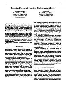
with 0 ≤ β ≤ 1 is the learning parameter. 2.1. Building Social Networks Social network is a social structure represented as a graph in which nodes represent objects and edges represent social interactions between pedestrians. The social interaction weights are based on our social similarity weight measure eq (2). Once the tracklets are obtained from the scene, we apply the spatio-temporal algorithm that produces a dense number of cuboids ς1 , ς2 , . . . , ςNr ×Nc ( 2 × 2, 4 × 4 or 8 × 8 depending on the scene characteristics) as well as the time windows Ω1 , Ω1 , . . . , ΩNΩ (cf. Fig. 1). Within each cuboid in each time window, we do the following: (1) Closeness centrality On a graph, a geodesic between two nodes is a path connecting the nodes with the smallest number of edges. The classical definition of the closeness centrality is (the inverse of) the average distance to all other nodes [16]. Since similar behaving tracklets need to be spatially close to each other, in addition to the social similarity measure, i.e. eq (2), we use the closeness centrality among connected tracklet nodes for pruning only: if similar tracklet nodes are spatially distant (threshold td ), their connecting edge is deleted. This is then followed by applying the connected component

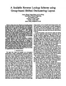
Fig. 1: System overview algorithm to the whole network. The idea is to identify the different dynamics of the scene, represented by the clusters in the network. We call each of these clusters obtained at this stage as local social network (LSN ). Local Social Network: A centroid is used to represent each LSN , denoted by CentSN i . It consists of the mean vector of its tracklets’ features, which are spatial < x, y >, direction φ, magnitude ρ, and velocity v. These LSN capture the local dynamics of each ςi . Global Social Network (GSN ): Once we obtain LSNi from the previous step, clustering is employed to have a coarser view of the scene. Our measure of the cluster centroid similarity is defined by eq (2). If similarity of two comparable social network’s centroid is sufficiently high, i.e. greater than a user-defined threshold tf , then the networks are merged together into one bigger network, otherwise they are reported as disjoint networks. For this, we perform Hierarchical Agglomerative Clustering [17]. Fig.1 illustrates the framework of our hierarchical clustering algorithm. Thus the merging is based on the social similarity measure as defined above - between and every two LSN components’ centroid, i.e. CentSN i of LSNi and LSNj , respectively. If the simCentSN j ilarity measure between LSNi and LSNj is above tf , they merge to form: GSNij = LSNi ∪ LSNj , and a new Cent for this is computed as well. This bottom-up approach aims to merge similar LSN s from different cuboids towards discovering the global social network GSNj within time window Ωk , thus capturing the dynamics of the whole window Ωi (cf. Fig 2).

Global Social Network per window

Merge local social network into global social network

global social network components within window

Local Social Network per cuboids

local social network components within cuboids

Partition the window into cuboids

s45 s56 s s21 46 s s s25 s42 s s1617s18 s535 51 1 2 22 s 50 0 s23 s s19 s12 53 s s13 41 s s2031 s14 s23 s34

s14 s12

s24

s33

s334s4 24

s11,12 s67

s1,14 s35 s8,99 s113,14s5,1 s31 s13,10 s29 s66,8 s12,14 s ,8 9,10 s13,14 s23 s10,14 s23,14 s47 s13 s3,7 s78 s36 s32

s122

s223

s7,9

s56 5 s455

s78

s99,10 ,1 10 0

s566

s3344

s12 s1133

s12 s344

s14

s2233

s67

Fig. 2: GSN per window obtained by grouping LSNi .

social network component in the neighborhood, it is classified as an anomalous local social network component. Global anomalies are detected in the similar way, using: GAςi =

GSNhΩi maxsize(GSNjΩi )

, 1 ≤ j ≤ n and j 6= h

if the relative size of the tested GSNhΩi is less than th % the size of the densest GSN component in the neighborhood maxsize(GSNjΩi ), it is classified as an anomalous. In summary, the method starts by determining the size of each social network component based on the number of its tracklets members. Then it determines the largest or densest social network in the neighborhood. The algorithm, hence, uses a threshold ta to differentiate each non-densest social network as normal or abnormal component. If the relative size of each tested social network component is less than th % the size of the densest social network component in the neighborhood then it is classified as an anomalous social network component.

2.2. Anomaly Detection Our social similarity measure, in addition to the size of social network, is considered an essential step for identifying abnormality. For each cuboid ςj , to identify which ς local social network component(s) LSNi j is anomalous, we use: ς

ςj

LA

LSNhj = ς , 1 ≤ i ≤ n and i 6= h maxsize(LSNi j )

Thus, if the relative size of the tested local social network component is less than th % the size of the densest local

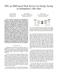
3. EXPERIMENTS & RESULTS We conducted an extensive set of experiments on the following crowd dataset: the UCSD pedestrian dataset. The dataset contains two sequences: UCSD Ped1, containing groups of people walking towards and away from the camera with some amount of perspective distortion, and UCSD Ped2, containing groups of people walking in parallel to the camera plane (cf. Fig. 3). Commonly occurring anomalies include small golf carts in the scene, skaters, bikes, and people in wheelchairs. Each scene

Fig. 3: Examples of anomaly detections using (col 1) the MDT approach[9], (col 2) the SF-MPPCA approach [9], (col 3) our detection approach and (col 4) our tracking results. For MDT, its abnormal detection foreground mask is too large thus its results are not accurate; and for SF-MPPCA, it inaccurately detects the small car (row 1), completely misses the bike in (row 2), completely misses the skater in (row 3) and produces spurious abnormality.

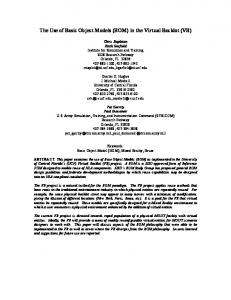
was divided into clips of about 200 frames, and resolution of 158 x 238 for UCSD Ped1 and resolution 360 x 240 for UCSD Ped2. Our proposed method run all the experiments on a PC computer with an Intel(R) Core(TM) i5−2400 3.10GHz CPU and 4GB RAM under the MATLAB implementation. For both sequences, the search window size for tracking is set to 16 x 16 pixels in the Lucas-Kanade based methods, with three pyramid levels, around 1000 foreground features and 4 as the minimum distance imposed between corner features. For the construction of feature vectors, we partition each 50 frames time window into 8 x 8 spatio-temporal cuboids. The values for α and β are chosen experimentally to be 0.8 and 0.4, respectively; and th % = 50%. We use the frame-level criterion: a frame is considered an anomaly if it contains at least one abnormal pixel, and denoted as positive. For the LSN, we measure the frame accuracy. For the global evaluation, we use the Receiver Operating Characteristic (ROC) curve, which is based on True Positive Rate (TPR) and False Positive Rate (FPR) [18]. Area under the curve(AUC) is computed from the ROC curve to compare our method to the other methods, as shown in Fig. 4, and compared in Table 1. Rate of Detection [9] is shown in Table 2. It is clear that our method clearly out performs the state-of-the-art methods. 4. CONCLUSION We present a general method that covers both local and global anomalous events without the need for back-

Fig. 4: ROC Curves: (top) Frame-level for UCSD-Ped1. (bottom) Frame-level for UCSD-Ped2.

UCSD-Ped1 UCSD-Ped2

MDT [9] 81.8% 84.8%

SRC [10] 86.0% 86.1%

Our Method 85.1% 87.0%

Table 1: Quantitative frame-level comparison using the AUC for our method and the state-of-the-art methods. localization

MDT [9] 45%

SRC [10] 46%

Our Method 47.4%

Table 2: The quantitative comparison of the detection rate (RD) at equal error for the anomaly localization task on UCSD Ped1. ground/foreground segmentation and individual tracking. We performed learning and tested on standard dataset and compared our results with the state-of-theart. The main advantages of our method are that it learns the dominant behavior in an unsupervised manner while simultaneously detecting anomalous patterns. Such characteristic of a visual surveillance system operates better in an unconstrained environment. 5. REFERENCES [1] A. Gritai A. Basharat and M. Shah, “Learning object motion patterns for anomaly detection and improved object detection,” in Computer Vision and Pattern Recognition. IEEE, 2008, pp. 1–8. [2] S. Ali and M. Shah, “Floor fields for tracking in high

density crowd scenes,” in Computer Vision-ECCV. IEEE, 2008, pp. 1–14. [3] A. Oyama R. Mehran and M. Shah, “Abnormal crowd behavior detection using social force model,” in Computer Vision and Pattern Recognition. IEEE, 2009, pp. 935–942. [4] A.D. Bue R. Raghavendra and M. Cristani, “Optimizing interaction force for global anomaly detection in crowded scenes,” in Computer Vision Workshops (ICCV Workshops). IEEE, 2011, pp. 136–143. [5] S. Ali and M. Shah, “A lagrangian particle dynamics approach for crowd flow segmentation and stability analysis,” in Computer Vision and Pattern Recognition. IEEE, 2007, pp. 1–7. [6] Z. Yi W. Chongjing, Z. Xu and L. Yuncai, “Analyzing motion patterns in crowded scenes via automatic tracklets clustering,” Communications, China 10, vol. 4, pp. 144– 154, 2013. [7] Y. Wu F. Jiang and A.K. Katsaggelos, “Detecting contextual anomalies of crowd motion in surveillance video,” in Conference on Image Processing (ICIP). IEEE, 2009, pp. 1117–1120. [8] Ed.P. Sparks M. J. V. Leach and N.M. Robertson, “Contextual anomaly detection in crowded surveillance scenes,” Pattern Recognition Letters, vol. 44, pp. 71–79, 2013. [9] W. Li V. Mahadevan and V. Bhalodia, “Anomaly detection in crowded scenes,” in Computer Vision and Pattern Recogniton (CVPR). IEEE, 2010, pp. 1975–1981. [10] J. Yuan Y. Cong and J. Liu, “Sparse reconstruction cost for abnormal event detection,” in Computer Vision and Pattern Recogniton (CVPR). IEEE, 2011, pp. 3449–3456. [11] Z. Qin and C.R. Shelton, “Improving multi-target tracking via social grouping,” in Computer Vision and Pattern Recogniton (CVPR). IEEE, 2012, pp. 1972–1978. [12] D. Lin D.J. Anderson P. Perona X.P. Burgos-Artizzu, P. Dollr, “Social behavior recognition in continuous video,” in Computer Vision and Pattern Recogniton (CVPR). IEEE, 2012, pp. 1322–1329. [13] T. Yu, K. Patwardhan S. Lim, and N.Krahnstoever, “Monitoring, recognizing and discovering social networks,” in Computer Vision and Pattern Recogniton (CVPR). IEEE, 2009, pp. 1462–1469. [14] J.Y. Bouguet, “Pyramidal implementation of the affine lucas kanade feature tracker description of the algorithm,” Intel Corporation, vol. 1, pp. 1–9, 2001. [15] D. Mitrovic M. Zeppelzauer, M. Zaharieva and C. Breiteneder, “A novel trajectory clustering approach for motion segmentation,” in Advances in Multimedia Modeling, 2010, pp. 433–443. [16] L.C. Freeman, “Centrality in social networks conceptual clarification,” Social networks, vol. 1, pp. 215–239, 1979. [17] E. Han G. Karypis and V. Kumar, “Chameleon: Hierarchical clustering using dynamic modeling,” Computer, vol. 8, pp. 68–78, 1999.

[18] Tom Fawcett, “An introduction to roc analysis,” Pattern Recognition Letters, vol. 27, pp. 861–874, 2006.