Intuitive Algorithms - CiteSeerX

Intuitive Algorithms

Von der Fakult¨at f¨ ur Mathematik, Informatik und Naturwissenschaften der RWTH Aachen University zur Erlangung des akademischen Grades eines Doktors der Naturwissenschaften genehmigte Dissertation vorgelegt von Diplom-Informatiker Joachim Kneis aus K¨oln

Berichter:

Prof. Dr. Peter Rossmanith Prof. Dr. Dieter Kratsch

Tag der m¨ undlichen Pr¨ ufung: 23.7.2009

Diese Dissertation ist auf den Internetseiten der Hochschulbibliothek online verf¨ ugbar.

ii

Abstract Assuming P 6= NP, which is widely believed to be true, many important computational problems are not solvable in polynomial time. However, this does not imply that NP-hard problems are not exactly solvable at all. Both the concepts of moderately exponential time algorithms and parameterized complexity provide tools for solving many of these problems in reasonable time. In this thesis, we introduce the concept of intuitive algorithms. While intuitive algorithms can be either moderately exponential time algorithms or parameterized algorithms, we require that they follow an intuitive idea and are kept as simple as possible. When we analyze algorithms only in terms of a worst case runtime bound, this approach is disadvantageous, as it is sometimes much harder to prove good bounds for simpler algorithms. In some cases, this might even be impossible. However, we will show that there are several aspects of intuitive algorithms that makes the development of such algorithms worthwhile. For example, their runtime is often not as bad as assumed. Especially on small instances, intuitive algorithms often outperform more complex algorithms, because the more complex algorithms tend to unfold their full potential on large instances. However, in practice large instances cannot be solved with exponential time algorithms at all. Furthermore, we often do to not know precise lower bounds on the runtime of exact algorithms. Is is thus hard to decide, whether more complex operations only ease the analysis of a complex algorithm or if such operations really improve the running time. Moreover, intuitive algorithms tend to allow for efficient implementations. This allows us to solve real life instances of surprisingly large size. In contrast to this, implementations of complex algorithms can be rather slow. Finally, intuitive algorithms are often more aesthetic than complex algorithms. Overall, simpler algorithms often tell us more about problems. Throughout this thesis, we will outline that intuitive algorithms can also be competitive when compared to traditional algorithms. To emphasize this, we will present several examples of intuitive algorithms that are either the fastest known algorithms or have only been improved recently.

List of Results • For Max-2SAT and Max-Cut, we present intuitive algorithms with a runtime bounded by O ∗ (1.128m ), where m denotes the number of clauses or edges, respectively. • For the Maximum Leaf Spanning Tree problem, we introduce an intuitive algorithm with a runtime bounded by O ∗ (4k ) that works both on

iii

undirected and directed graphs. Here, the parameter k denotes the number of leaves. • We show that Partial Vertex Cover can be solved with an deterministic intuitive algorithm in time O ∗(1.396t ) and with a less intuitive randomized algorithm in time O ∗ (1.2993t), where t is the number of covered edges. • Moreover, we present an algorithm for Partial Dominating Set with a runtime bounded by O ∗ ((4 + ε)t ), which is based on the technique of Divide & Color. Here t denotes the number of dominated nodes. • Finally, we present an intuitive algorithm for Independent Set with a runtime bounded by O ∗ (1.2132|V | ). The first and the last result thereby are moderately exponential time algorithms, while our algorithms for Maximum Leaf Spanning Tree, Partial Vertex Cover, and Partial Dominating Set are parameterized algorithms. The focus in this thesis lies on proving the claimed theoretical runtime bounds for these algorithms. However, we will also present implementations for each algorithm and argue that they can be used to solve surprisingly large instances.

iv

Acknowledgments My first and sincere thanks go to my supervisor Professor Peter Rossmanith for his wise guidance, his unstoppable enthusiasm for new ideas, his deep insights into algorithms and complexity as well as his valuable advice on exotic food. Without his foresight, patience and trust in me, I might not have come to this point. Furthermore, my warmest thanks go to all the members (former and present) of the Lehr- und Forschungsgebiet Theoretische Informatik at RWTH Aachen University, for sharing ideas and a great working atmosphere: Daniel M¨olle, Alexander Langer and Stefan Richter. Working together with them was both entertaining and enlightening. Many thanks for the invitation to ETH Z¨ urich and the hospitality to Professor Juraj Hromkovic and my other co-workers at the Chair of Information Technology and Education: Hans-Joachim B¨ockenhauer and Joachim Kupke. Moreover, I would like to thank all of my co-authors (in alphabetical order): Hans-Joachim B¨ockenhauer, Henning Fernau, Luca Forlizzi, Jens Gerlach, Juraj Hromkovic, Joachim Kupke, Dieter Kratsch, Daniel M¨olle, Alexander Langer, Mathieu Liedloff, Guido Proietti, Daniel Raible, Stefan Richter, Peter Rossmanith, and Peter Widmayer for sharing their knowledge and expertise with me. They all greatly contributed to the successful completion of this dissertation. Last but not least, I want to thank my parents and my wife Anne for their support and help throughout all these years.

This thesis was funded by the German Research Foundation (DFG) under the project RO 927/7.

v

vi

Contents 1 Introduction 1.1 Exact Algorithms . . . . . . . . . . . . . . . . . . . . . . . . . . . . 1.2 Intuitive Algorithms . . . . . . . . . . . . . . . . . . . . . . . . . . 1.3 Preliminaries . . . . . . . . . . . . . . . . . . . . . . . . . . . . . .

1 2 3 6

2 MaxCut and Max2SAT 2.1 Previous Results . . . . . . . . . . . . . . . . . . . 2.2 A Confluent Set of Reduction Rules . . . . . . . . . 2.3 Bounds on Treewidth and Pathwidth . . . . . . . . 2.4 A General Framework for Intuitive Algorithms . . . 2.4.1 Algorithms for Max-2SAT and Max-Cut 2.5 Implementation . . . . . . . . . . . . . . . . . . . . 2.6 Concluding Remarks . . . . . . . . . . . . . . . . .

. . . . . . .

. . . . . . .

. . . . . . .

. . . . . . .

. . . . . . .

. . . . . . .

. . . . . . .

. . . . . . .

. . . . . . .

9 10 12 19 26 31 36 43

3 Maximum Leaf Trees 3.1 Previous Results . . 3.2 Preliminaries . . . . 3.3 The Algorithm . . . 3.4 Implementation . . . 3.5 Concluding Remarks

. . . . .

. . . . .

. . . . .

. . . . .

. . . . .

. . . . .

. . . . .

. . . . .

. . . . .

45 47 49 52 59 62

. . . . . . . .

65 67 67 70 76 78 83 85 88

. . . . .

. . . . .

. . . . .

. . . . .

. . . . .

. . . . .

. . . . .

. . . . .

4 Partial Vertex Cover 4.1 Previous Results . . . . . . . . . . 4.2 Preliminaries . . . . . . . . . . . . 4.3 A Fast Algorithm on Cubic Graphs 4.4 A deterministic algorithm . . . . . 4.5 A randomized algorithm . . . . . . 4.6 Exact Partial Vertex Cover 4.7 Implementation . . . . . . . . . . . 4.8 Concluding Remarks . . . . . . . .

. . . . . . . . . . . . .

. . . . . . . . . . . . .

. . . . . . . . . . . . .

. . . . . . . . . . . . .

. . . . . . . . . . . . .

. . . . . . . . . . . . .

. . . . . . . . . . . . .

. . . . . . . . . . . . .

. . . . . . . . . . . . .

. . . . . . . .

. . . . . . . .

. . . . . . . .

. . . . . . . .

. . . . . . . .

. . . . . . . .

. . . . . . . .

. . . . . . . .

5 Partial Dominating Set 91 5.1 Previous Results . . . . . . . . . . . . . . . . . . . . . . . . . . . . 91 5.2 A Problem Kernel for Partial Dominating Set . . . . . . . . . 92

vii

Contents 5.3 5.4 5.5 5.6

A Randomized Algorithm for Partial Dominating Set Derandomization . . . . . . . . . . . . . . . . . . . . . . . Implementation . . . . . . . . . . . . . . . . . . . . . . . . Concluding Remarks . . . . . . . . . . . . . . . . . . . . .

6 Independent Set 6.1 Previous Results . . . . . . . . . . . . . . . . . . . . . . . 6.2 An Intuitive Algorithm . . . . . . . . . . . . . . . . . . . . 6.3 Sparse Graphs . . . . . . . . . . . . . . . . . . . . . . . . . 6.3.1 Runtime Analysis . . . . . . . . . . . . . . . . . . . 6.4 Arbitrary Graphs . . . . . . . . . . . . . . . . . . . . . . . 6.5 A Computer Aided Case Distinction . . . . . . . . . . . . 6.5.1 A General Framework for Computer Aided Proofs . 6.5.2 Generating all Graphlets of maximum Degree Four 6.6 A Traditional Analysis of the Remaining Cases . . . . . . . 6.7 Implementation . . . . . . . . . . . . . . . . . . . . . . . . 6.8 Concluding Remarks . . . . . . . . . . . . . . . . . . . . .

. . . . . . . . . . . . . . .

. . . . . . . . . . . . . . .

. . . . . . . . . . . . . . .

. . . .

. . . .

94 100 103 106

. . . . . . . . . . .

107 . 108 . 109 . 114 . 117 . 127 . 128 . 128 . 129 . 135 . 140 . 144

7 Conclusion

147

Bibliography

149

A Tree- and Pathwidth: Basic Definitions

161

B Implementation Details 163 B.1 Maximum Leaf Spanning Tree . . . . . . . . . . . . . . . . . . . . . 163 B.2 Partial Vertex Cover . . . . . . . . . . . . . . . . . . . . . . . . . . 165 B.3 Independent Set . . . . . . . . . . . . . . . . . . . . . . . . . . . . . 167

viii

1 Introduction One of the fundamental concepts in computer science is the classification of computational problems according to their complexity. Probably the most important aspect of this classification is that it allows us to describe which problems are efficiently solvable. Traditionally, all problems contained in P, i.e., problems that can be solved in polynomial time, belong to this category, whereas all NP-hard problems are usually considered to be not efficiently solvable. Unfortunately, many problems fall into the second category. For example, Garey and Johnson [63] listed over 300 NP-hard problems in their guide to NP-completeness as early as in 1979. Since then the number of NP-hard problems has increased dramatically. Today, it is widely believed that there are least several thousand natural NP-hard problems. Among these vast number of problems are both problems that are relevant in practice and problems that are of purely theoretical interest. A real life example of an NP-hard problem is the so called 3-Dimensional Packing problem: given a set of three dimensional boxes and a set of containers, we have to decide whether all boxes fit into the containers. Optimization variants of this problem are obviously important in practice. On the other hand, a purely theoretical problem that is NP-hard is the Short Turing Machine Acceptance problem, which asks whether a given Turing machine accepts a word after at most k steps1 . Other wellknown hard problems are, e.g., Hamiltonian Circuit, Independent Set, and 3-Coloring (see, e.g. [63]). Assuming P 6= NP, none of these problems admits a polynomial time algorithm. However, it is widely accepted that these problems need to be tackled somehow. This led to the development of several techniques for solving such hard problems. The simplest techniques are heuristics. These algorithms usually run very fast and perform well on real life instances. Their drawback is that they do not guarantee any fixed runtime bound and do not necessarily return the correct output, but do so only on many instances. While this might be only a minor nuisance in practice, it is usually not acceptable from a theoretical point of view. Among those concepts that are accepted in our theoretical community, approximation and randomization are probably the most important polynomial time methods. While randomized (polynomial time) algorithms are allowed to return a wrong 1

k is given as a unary number

1

1 Introduction solution, they are required to fail only with a small probability. The runtime of other variants of randomized algorithms depends on some random variable. In contrast to heuristics, the uncertainty in randomized algorithms is bounded by some proven bound. For an introduction into randomized algorithms, we refer the reader to the monograph by Motwani and Raghavan [97]. However, it is very unlikely that randomized algorithms can be used to solve NP-hard problems in polynomial time [125]. Approximation algorithms are applied to optimization problems, which ask to find an optimal solution instead of only deciding whether the answer is “yes” or “no”. Instead of returning the optimal solution, approximation algorithms return a solution that is not necessary optimal but within a well-defined distance from the optimal solution. See Vazirani [127] for an introduction into approximation algorithms. Unfortunately, approximated results are not always sufficient. Approximation factors of large constants — in some cases even a factor of 2 — are not necessarily useful [86]. Moreover, many problems, including Independent Set and Dominating Set, can not be approximated with a constant approximation ratio unless P = NP [71, 108].

1.1 Exact Algorithms A paradigm that can be broadly applied is the development of moderately exponential time algorithms. At the cost of exponential runtime bounds, such algorithms guarantee to return the correct (or an optimal) solution regardless whether the input instance is well formed or not within guaranteed runtime bounds. The focus in the design of such exact algorithms is to keep the exponential runtime as small as possible, because otherwise even small instances cannot be solved. Typically, this means runtime bounds of the form cn · p(n), where n is the input size, c is a small constant (preferable c < 2) and p is a polynomial. The disadvantage of this concept is of course that it can only be applied to solve small problem instances. However, moderately exponential time algorithms are surprisingly successful. Independent Set and Dominating Set for example, which can not be approximated with a small approximation ratio unless P = NP as mentioned above, both allow for fast exact algorithms. Dominating Set can be solved in time O ∗ (1.5134n )2 [126] and Independent Set can be solved in time O ∗ (1.22n ) [56] (for an improvement of the latter runtime bound, see Chapter 6). While the last years saw some huge improvements in the field of exact algorithms, the focus of this research lies mostly on developing algorithms with the best asymp2

2

The O∗ -notation suppresses polynomial factors in the runtime.

1.2 Intuitive Algorithms totic runtime bounds. Since the asymptotic runtime is largely dominated by the exponential factors, runtimes are considered better, if these factors are smaller. The polynomial factors usually play only a minor role in the design of exact algorithms. The widespread use of the O ∗ -notation instead of the O-notation gives the best proof to this.3 Related to the topic of moderately exponential time algorithms is the field of parameterized complexity (see e.g. [45, 54, 100] for an introduction). While both areas are devoted to the exact solution of hard problems, parameterized complexity asks for algorithms whose runtime is only exponential in a parameter but not in the input size. Such algorithms, for example an algorithm with a runtime bounded by O(2k n2 ) for parameter k and input size n, are called fpt-algorithms (derived from fixed parameter tractable). This bears the potential of very fast algorithms, as long as we try to solve problems with small parameters only. However, many parameterized algorithms are only developed to prove that some problem is fixed parameter tractable, and thus do not use the full potential of this concept. Nevertheless, it seems only natural to consider both kind of exact algorithms also in practice, since the exponential parts in runtime bounds of exact algorithms become smaller and smaller. Some examples already show that exact algorithms can be used to solve real life input instances. For instance, Langston, Perkins, Saxton, Scharff and Voy used algorithms for Clique and Vertex Cover to evaluate how cells respond to radiation [86]4 . As another example, Gramm, Guo, H¨ uffner and Niedermeier [65] applied parameterized algorithms for the Clique Cover problem to solve some real life instances from statistical applications [106].

1.2 Intuitive Algorithms In this thesis, we follow this line to develop exact algorithms that are not only fast in terms of a theoretical analysis. We do not require that our algorithms can be immediately applied to large real life instances, since this would require that they are competitive with highly specialized tools like SAT solvers, see e.g., [67, 107]. Instead, we require that they can be used as base algorithms that might be extended to be competitive. Of course, this implies that even the base algorithms should be able to solve real life instances of reasonable size. Thereby, we emphasize 3

We will use the O∗ -notation in thesis only when comparing results and present a precise analysis using the O-notation for each of our algorithms. 4 Note that although the title of this paper suggest a purely parameterized algorithm, the resulting algorithm is not an fpt-algorithm. The authors apply methods from parameterized complexity to improve an exact algorithm for Clique so that it can be applied to real life inputs.

3

1 Introduction that our algorithms are designed to be applicable in real life instance and yield good theoretical bounds at the same time. This contrasts the traditional approach, where algorithms are only designed to yield good theoretical bounds and it is considered only a slight surplus if they can be applied in real life as well. We believe that the increasing importance to solve hard computational problems exactly, e.g., in computational biology or medicine, justifies this approach. Compared to a purely theoretical analysis restricted to asymptotic runtime bounds, ensuring practical performance requires an approach that accounts for several other factors. Improving the exponential parts in the runtime bounds is of course a necessary condition to obtain efficient exact algorithms. Unfortunately, a good asymptotic worst case bound on the runtime does not guarantee that the algorithm is indeed efficient. First of all, the polynomial factors in the runtime bound cannot be neglected. While an O(1.4n n5 ) algorithm is asymptotically faster than an O(1.5n n2 ) algorithm, the latter performs better on instances of size n ≤ 230. But on instances of this size, both algorithms need more than 1045 steps, thus rendering them completely useless on such large instances. Therefore, the asymptotically slower algorithm should be preferred in this example.5 Furthermore, the effectiveness of an algorithm is not only determined by its proven upper bound. The proven runtime bounds for most algorithms are only a more ore less accurate estimations of the real runtime bound. For those algorithms, for which non-trivial lower bounds are known, there is usually a large gap between the upper and the lower bound, see e.g. [2, 56]. That is, a more evolved algorithm may admit a better provable upper bound, but is not clear, if its runtime is in fact better. In the majority of cases, more complex algorithms will probably have a better asymptotic runtime, but the exact advance will remain unclear. Moreover, improved theoretical upper bounds are often only achieved by more complex algorithms. While these may have better asymptotic runtimes — both theoretical and de-facto — their performance on real life instances may be very different. For most exact algorithms, no analysis for average-time complexity measures exist. Easier but (in the worst case) slower algorithms may perform better on almost all instances and might thus be preferable (see Chapter 6). Finally, modifying algorithms with techniques used in heuristics often speed up the computation but do not improve the theoretical upper bounds. Although such modifications can results in dramatically better performance on real life instances, their application is thus usually not considered in theoretical algorithms. Unfortu5

4

The klam-value, introduced by Downey and Fellows [45], is closely related to this analysis. It measures which instance sizes are solvable in 1020 by a given algorithm.

1.2 Intuitive Algorithms nately, more complex algorithms tend to hinder such modifications, see Chapter 4 for an example of this effect. Within our research, we found that the algorithms that perform very well under the criteria above are those algorithms that are based on an intuitive idea and are otherwise kept as simple as possible. Such intuitive algorithms need to be • as simple as possible and • competitive in terms of asymptotic runtime bound. Intuitive algorithms can often avoid the aforementioned problems of traditional algorithms. Since they are simple, their runtime bounds usually do not contain large polynomials or large hidden constants. Most exact algorithms repeat a rather short function very often, be it because of recursion, because of dynamic programming or because amplification of the success probability in the case of randomized algorithms. The repeated functions tend to be short in intuitive algorithms, which implies less effort in each call. In contrast to this, single recursive calls in traditional algorithms can be very complex, for example due to large case distinctions. The required simplicity in general also guarantees that the average runtime of intuitive algorithms is very good. Most algorithms use complex subroutines only to overcome some hard cases. However, these hard cases usually occur seldom, which renders the positive effect of such improvements very small in the average case. As a consequence, large case distinctions or other complex routines introduced to obtain a better asymptotic bound tend to be mostly ballast on real life instances. Intuitive algorithms thus often perform as least as good as traditional algorithms on real life instances (see Chapter 6). Furthermore, intuitive algorithms can easily be modified to improve the efficiency on real life instances. For example, many intuitive algorithms use recursion, which can easily be turned into a Branch & Bound method. In Chapter 4, we present an example where a complex algorithm (with an improved runtime) cannot be modified by such means and thus performs worse than a modified intuitive algorithm. However, an algorithm can be very simple but very slow both in practice as well as with respect to asymptotic upper bounds. Since a worst case analysis is still a very good indicator for the runtime of an algorithm, we thus require that the runtime of an intuitive algorithm is at least close to the fastest known algorithms. As a consequence, intuitive algorithms tend to perform well on real life instances. Of course, the requirements of being simple and being fast often compete with each. Thus, an intuitive algorithm is often subject to a trade-off between simplicity and efficiency. In this thesis, we will try to give enough evidence, that it is possible and worthwhile to develop such intuitive algorithms. On that account, we present several case studies, each containing one ore more intuitive algorithms for some

5

1 Introduction computational problem. Since this thesis originates from a theoretical background, the focus within each case study thereby still lies on the theoretical analysis and the obtained upper bounds. However, each case study also includes some arguments why the algorithms can be considered intuitive. For this reason, each case study contains a section that describes how the respective algorithms can be implemented and how they perform on real life instances. Our goal is to give some examples, where intuitive algorithms are both fast in terms of a traditional analysis but at the same time also efficient on real life instances. This thesis is organized as follows: Section 1.3 presents some notations and concepts used in the design of exact algorithms. Chapters 2 to 6 each cover the application of intuitive algorithms to a specific problem. Chapter 2 discusses upper bounds on the treewidth of sparse graphs and its applications to Max-Cut and Max-2SAT. Chapter 3 deals with the Maximum Leaf Spanning Tree problem, Chapter 4 with the Partial Vertex Cover problem and Chapter 5 with the Partial Dominating Set problem. Finally Chapter 6 presents some results on the Independent Set problem.

1.3 Preliminaries We assume the reader to be familiar with the O-notation. The O ∗ -notation is slightly stronger, as it suppresses all polynomial factors. For example, O(2n n3 ) ⊆ O ∗ (2n ). Note that we follow the common but formally incorrect notion of using these sets as functions, i.e., we write a runtime “is bounded by O(2n n3 )” instead of a runtime “is contained in O(2n n3 )” and allow notions like T (n) = O(2n n3 ), where T (n) is a function in n. Definition 1.1 Let f : N → N be a function, and g : N × N → N, h : N × N → N be polynomials. Then we denote O(f (k)g(n, k) + h(n, k)) by O ∗ (f (k)). For the sake of brevity, we define the following symbols and abbreviations for graphs G = (V, E). As usual, we let n and m denote the number of nodes and edges in a graph, respectively. By V (G) and E(G) we denote the set of nodes and the set of edges in G. Moreover, the maximum (minimum) degree of G is denoted by ∆(G) (δ(G)). We also abbreviate three-regular graphs as cubic graphs. If U ⊆ V , then G[U] denotes the subgraph of G induced by U. In a slight abuse of notation, we abbreviate G[V \ U] as G \ U. We denote by N(v) := { u ∈ V | (v, u) ∈ E } the set of all neighbors of v ∈ V , S and N[v] := N(v) ∪ {v}, and for U ⊆ V we let N[U] := u∈U N[u] as well

6

1.3 Preliminaries
S as N(U) = N[U] \ U. Moreover, we define N i+1 [u] := N[N i [u]] and u∈U i+1 i+1 i N (u) := N [u] \ N [u] for i ≥ 1 (N i+1 [U] and N i+1 (U) accordingly). We will postpone the introduction of notions that are only used once to the corresponding chapters. In the following, we will often analyze recursive algorithms that compute a solution based on solutions of smaller instances. Such algorithms often try several possible conditions, for example, each possible coloring of a given node in 3-Coloring, and then proceed in each branch recursively using the gained information. We will call such algorithms in the following branching algorithms. As it is not clear which branch yields the correct solution, we have to follow all branches and hence typically obtain an exponential runtime bound. We will denote a single step where an algorithm uses several recursive calls a branching step or simply a branch. A description of which recursive calls need to executed is called branching rule. We refer the reader to the monograph by Niedermeier [100] for a detailed introduction into this topic. Note that a branching algorithm A always implies a recursive search tree TA , where each node in TA a call in the algorithm. Since the time spend in each call is often polynomial and easy computable, bounding the size of TA is often sufficient to obtain a overall runtime bound for A. In general, we will compute an α such that the number of leaves in TA is bounded by α|I| , when A is called on a instance I. IfPthe branching on I yields the new instances I1 , . . . , It , this implies that α|I| ≥ ts=1 α|Is| . Branching Vectors are a helpful tool in such an analysis. Definition 1.2 Let A be a branching algorithm that calls itself on an instance I on smaller instances I1 , . . . , It . Let ∆i = |I|−|Ii |. Then (∆1 , . . . , ∆t ) is a branching vector of A. For any branching vector B = (∆1 , . . . , ∆t ), we denote by αB the minimal value P |I| |I | such that αB ≥ ts=1 αBs . Note that |I| can be the input size, but can also be the size of a parameter or any other measure. Moreover, note that the ∆i are not necessarily integers. Especially when using the Measure & Conquer approach by Fomin, Grandoni, and Kratsch [56], these values tend to be rational numbers. Obviously, we want to minimize α. If each branching step of an algorithm A implies the same branching vector B, the number of leaves in TA is bounded by αB . Unfortunately, each branching step of an algorithm can imply a different branching vector. But then, |TA | is bounded by the maximal αB for all occurring

7

1 Introduction branching vectors B (see [100]). The following theorem allows us to efficiently compute αB for a given branching vector. Theorem 1.3 (cf., Niedermeier [100]) Let B = (∆1 , . . . , ∆t ) be a branching vector and let d = max ∆i . Then, αB ≤ α, where α is the unique positive real root of the characteristic polynomial χ(z) = z d − z d−∆1 − . . . − z d−∆t α is called branching number of B. In the following, we will usually give only the branching vectors of an algorithm and the resulting branching number. The evaluation of the characteristic polynomial is technical and will be skipped, as it can easily be computed automatically with sufficient accuracy. In Chapter 4, we will explicitly compare branching vectors according to their branching number. The following relation on branching vectors will be helpful in this: let s = (s1 , . . . , sl ) and t = (t1 , . . . , tl ) be two branching vectors of equal length. We say s dominates t (denoted by s D t or t E s), iff s1 ≥ ti for 1 ≤ i ≤ l. If s D t, then the branching number for s is obviously smaller than the branching number for t. For more information about branching vectors and the corresponding branching numbers, see [100].

8

2 MaxCut and Max2SAT In this chapter, we present an upper bound on the pathwidth1 of graphs with respect to the number of edges as well as an polynomial time algorithm to compute a corresponding path decomposition. Moreover, we present intuitive algorithms for Max-Cut and Max-2SAT based on this result. These problems are defined as follows: Max-2SAT Input: A CNF formula, such that each clause contains at most two literals and a positive integer k Question: Is there assignment to the variables that satisfies at least k clauses? Max-Cut Input: A graph G = (V, E) and a positive integer k Question: Is there a partition V1 ∪ V2 = V such that |{ {u, v} ∈ E | u ∈ V1 , v ∈ V2 }| ≥ k? While the tree- and pathwidth of a graph is a well-studied measure in the design of exact algorithms, see e.g. [1, 19, 38, 42, 123], no non-trivial upper bounds for arbitrary graphs with respect to the the number of edges were discovered for those measures. Here, we present such a bound by introducing a polynomial time algorithm that computes a path decomposition of size m/5.769 + O(log(n)). This algorithm simply removes a node v of maximum degree from the graph and computes a path decomposition P for the remaining graph recursively. Afterwards, v is added to each bag of P. If the maximum degree decreases to at most three, we use an algorithm by Fomin and Høie [59] to compute a path decomposition of size about n/6. Together with some straightforward reduction rules, this is sufficient to obtain the claimed bound. While this is an important graph-theoretical result by itself, this immediately improves the runtime bounds for some well-known problems. Using the framework by Telle and Proskurowski [123], we obtain runtime bounds of O ∗ (2m/5.769 ) for 1

We assume that the reader is familiar with the notions of tree- and pathwidth. An explanation of terms relevant to this thesis can be found in the appendix. For a detailed introduction, we refer the reader to the surveys by Bodlaender [17] and Kloks [77].

9

2 MaxCut and Max2SAT Max-2SAT and Max-Cut, where m denotes the number of clauses in the case of Max-2SAT. However, the resulting algorithms rely on dynamic programming and hence require exponential space. Moreover, the algorithm by Fomin and Høie is based on a method by Monien and Preis [94] that computes a small separator in cubic graphs. However, this method is rather complicated and thus the resulting algorithms cannot be considered intuitive. Nevertheless, using the algorithm outlined above but avoiding the special algorithm for cubic graphs allows us to compute a tree decomposition of size m/5.217 + 3. Due to the very simple strategy applied in this construction, the resulting decomposition can be used to solve Max-Cut and Max-2SAT without dynamic programing at all. In fact, we present algorithms for Max-Cut and Max-2SAT that do not explicitly construct the decomposition but use its structure in an branching algorithm. This yields intuitive algorithms for both problems with a runtime bounded by O ∗ (2m/5.217 ) using only polynomial space. Furthermore, this concept can be used as a framework to develop algorithms for other hard problems, as long as some simple conditions are satisfied. More precisely, the algorithms described in this chapter operate on a graph representation ϕ(I) of the respective instance I (such as the connectivity graph of a 2SAT formula or the graph itself in case of Max-Cut). Nodes of degree at most two are removed according to a simple set of reduction rules. If no such nodes exist, the algorithms select and remove nodes of maximum degree iteratively until the graph becomes series-parallel. In general, it does not make a difference which node of maximum degree is selected, except for the four-regular case: it is vital to avoid cases where a degree-four node has only neighbors of degree four whenever this is possible. A problem can be solved by our framework if all these graph operations correspond to appropriate operations in the problem instance. On the one hand, there need to be corresponding reduction rules for I whose application allows us to remove nodes of degree at most one and contract nodes of degree two in ϕ(I). On the other hand, we need to deal with arbitrary nodes of high degree in ϕ(I). Typically, simply branching on I will result in the removal of a node in ϕ(I), which then leads to the exponential runtime bounds.

2.1 Previous Results Until now, there has been few research on the path- and treewidth of sparse graphs. The only — to our best knowledge — result was obtained by Fomin and Høie, who presented an upper bound of (1 + ε)n/6 + O(log n) on the pathwidth of cubic

10

2.1 Previous Results graphs with n nodes [58, 59]. However, this field is related to the Maximum Induced Planar Subgraphpproblem [96]: The treewidth of any planar graph with t nodes is bounded by O( (t)). Hence, we can remove all nodes that do not belong to a maximum induced planar subgraph to obtain a tree decomposition of p size n − t + O( (t)). An algorithm by Edwards and Karr [46] uses a strategy very similar to the one applied later on in order to find maximum induced planar subgraphs of size (d − 2)/(d + 1)n, where d is the average degree of a given graph. Since this algorithm does not yield an arbitrary induced planar subgraph but even a planar subgraph of treewidth two, this yields the slightly worse bound of m/5 + 2 on the treewidth. There are however various exact algorithms for Max-Cut and Max-2SAT. For Max-2SAT, Niedermeier and Rossmanith [102] developed an algorithm with a runtime of O ∗ (2m/2.88 ). Subsequent improved algorithms are due to Bansal and Raman [10] (O ∗ (2m/3.44 )) as well as Fedin and Kulikov [48] (O ∗(2m/4 )). Moreover, Gramm, Hirsch, Niedermeier, and Rossmanith [66] obtained an bound of O ∗ (2m/5 ). All of these results also imply algorithms for Max-Cut by the standard reduction from Max-Cut to Max-2SAT, which unfortunately creates two clauses for each edge. However, none of the algorithms above can be considered intuitive, as they all require complex branching and reduction rules. The O ∗ (2m/5 ) algorithm for Max-2SAT [66], for example, employs six reduction rules as well as a six-fold case distinction. Lately, several authors have matched or improved our aforementioned bounds. Using an argument based on linear programming, Scott and Sorkin presented an alternative proof for the bound of m/5.769+O(log n) on the treewidth (in fact, their type-III reduction selects nodes in roughly the same way as our algorithm) [117]. Again, this result leads to runtime bounds of O ∗(2m/5.769 ) for Max-2SAT and Max-Cut. Using a similar approach, they also obtained an O ∗ (2m/5.263 ) algorithm for Max-2SAT and Max-Cut using only polynomial space [116], improving on our bound of O ∗(2m/5.217 ). Note that a technical report published shortly before our result already contains this m/5.263 bound [115].2 Kojevnikov and Kulikov have taken the runtime bound for Max-2SAT under polynomial space restrictions to O ∗ (2m/5.5 ) [82], which was subsequently improved to O ∗ (2m/5.88 ) by Kulikov and Kutzkov [85]. Their algorithm uses a structure similar to our algorithm: first the formula is reduced by simple reduction rules, then they branch on a variable. In order to achieve the improved runtime bounds, Kojevnikov and Kulikov simulate branching on every variable and select the best one for the real branching process, whereas we always select some node of maxi2

As pointed out by Scott and Sorkin, these bounds can easily be expanded into bounds of O∗ (rm/5.263 ) and O∗ (rm/5.217 ) for Max-2CSP with r-ary variables.

11

2 MaxCut and Max2SAT mum degree. However, the additional quadratic factor in the runtime cannot be neglected for practical instances. It is thus questionable whether this algorithm can be considered intuitive. Finally, Gaspers and Sorkin [64] improved the upper bound for Max-2SAT to O ∗ (2m/6.32 ). Again, this algorithm uses a complex case distinction and cannot be considered intuitive. In 2005, Williams developed an algorithm for Max-2SAT with a runtime bound of only O ∗(22.376n/3 ), depending on fast matrix multiplication. This is the currently fastest algorithm analyzed in the number n of variables [128]. As for approximation results, we refer the reader to [73, 90].

2.2 A Confluent Set of Reduction Rules The upcoming section introduces the reduction rules on graphs that are to play a crucial role throughout this chapter. Definition 2.1 Let G = (V, E) be a graph and let D ⊆ V be an arbitrary subset of its nodes. We define the following reduction rules: R0 : If there is a v ∈ / D with deg(v) = 0, then remove v from G, i.e., set G = G \ {v}. R1 : If there is a v ∈ / D with deg(v) = 1, then remove v from G. R2 : If there is a v ∈ / D with deg(v) = 2, then contract v, i.e., remove v from G and insert a new edge between its two neighbors, if no such edge exists. RD : If G contains a node v ∈ D, then remove v. R: If any of the above rules can be applied, do so. R∗ : Iterate R as long as possible. Note that RD is not a reduction rule in the classical sense. Whenever we remove a node by this rule, the width of the constructed decomposition increases by one. However, we need to prove that removing nodes and applying the other reduction rules in an arbitrary (but valid) order always yields the same graph in order to obtain our bound on the pathwidth. For the sake of readability, we thus incorporate the rule RD into our reduction rules, so that we only need to show that R∗ always yields the same graph. Definition 2.2 Let G = (V, E) be a graph, let D ⊆ V , and let v ∈ V be a node that can be reduced according to R0 , R1 , R2 , or RD . Then v is called reducible

12

2.2 A Confluent Set of Reduction Rules and Ghvi denotes the graph obtained from G by applying the respective rule on v. For r ≥ 2 we define Ghv1 , . . . , vr i = Ghv1 ihv2 , . . . , vr i inductively. If vi is reducible in Ghv1 , . . . , vi−1 i for all 1 ≤ i ≤ r then (v1 , . . . , vr ) is a valid reduction sequence for G with respect to D. By ε we denote the (valid) empty reduction sequence. Given two valid reduction sequences σ = (v1 , . . . , vr ) and τ = (v1′ , . . . , vs′ ), we set στ = (v1 , . . . , vr , v1′ , . . . , vs′ ), if {v1 , . . . , vr } ∩ {v1′ , . . . , vs′ } = ∅. In a slight abuse of notation, we define σ ∩ τ = {v1 , . . . , vr } ∩ {v1′ , . . . , vs′ }. Note that each valid reduction sequence (v1 , . . . , vr ) does not only describe which nodes are reduced according to some rule, but also describes which rule is applied, since exactly one reduction rule can be applied to each vi in Ghv1 , . . . , vr i. Moreover, we can obviously split Ghv1 , . . . , vr i at an arbitrary position i and obtain Ghv1 , . . . , vr i = Ghv1 , . . . , vi ihvi+1 , . . . , vr i. Whereas the rules are very simple, we need a few technical arguments to show that the order in which reductions are performed does not affect the outcome. See Figure 2.1 for an example. Lemma 2.3 Let G = (V, E) be a graph, let D ⊆ V , and let x, y ∈ V with x 6= y be two reducible nodes. Then (x, y) and (y, x) are valid reduction sequences for G and Ghx, yi = Ghy, xi. Proof. Deleting or contracting x does not affect the degree of y and vice versa if they are not adjacent. Then (x, y) and (y, x) are both valid reduction sequences and it is easy to see that Ghx, yi = Ghy, xi. If x and y are adjacent, then the application of a reduction rule to x or y either does not change the degree of the other node or decreases it by one. That is, the reduction of x or y cannot render the reduction of the respective other node impossible. Hence, (x, y) and (y, x) are valid reduction sequences. If none of the nodes are reduced according to R2 , it is also easy to see that Ghx, yi = Ghy, xi because the resulting graph is G \ {x, y}. Otherwise, we may assume that x is reduced by R2 without loss of generality. Since x and y are adjacent, y satisfies deg(y) ≥ 1. The remaining cases are depicted in Figure 2.2.  Lemma 2.4 Let G = (V, E) be a graph, let D ⊆ V , and let (v1 , . . . , vr ) be a valid reduction sequence for G such that vr is also reducible in G. Then (vr , v1 , . . . , vr−1 ) is also a valid reduction sequence for G, and Ghv1 , . . . , vr i = Ghvr , v1 , . . . , vr−1 i.

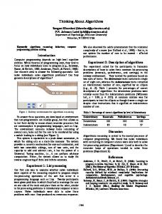
13

2 MaxCut and Max2SAT v0

v1 v2 v3 v4 v5 v6 v7

Ghv0 i

Ghv0 , v3 i

Ghv0 , v3 , v7 i

Ghv3 i

Ghv0 , v7 i

Ghv7 i

Ghv3 , v7 i

Ghv0 , v6 , v7 i

Ghv6 , v7 i

Ghv3 , v6 , v7 i

R∗ (G)

Figure 2.1: The above graphs illustrate the confluence of the reduction rules R1 and R2 : No matter in which order nodes of degree one or two are reduced, the outcome is always the same. The rule R0 cannot be applied because there are no isolated nodes, and we assume D = ∅ for the sake of readability. Proof. The claim is obvious for r ≤ 1 and given by Lemma 2.3 for r = 2. We show the cases r > 2 by induction on r. Recall that (v1 , . . . , vr ) is a valid reduction sequence for G and therefore (vr−1 , vr ) is a valid reduction sequence for Ghv1 , . . . , vr−2 i. In particular, vr−1 is reducible in Ghv1 , . . . , vr−2 i. Since vr is also reducible in G, it must also be reducible in Ghv1 , . . . , vr−2 i as well. Thus, Lemma 2.3 guarantees that (vr , vr−1 ) and (vr−1 , vr ) are valid reduction sequences for Ghv1 , . . . , vr−2 i and that Ghv1 , . . . , vr−2 ihvr−1, vr i = Ghv1 , . . . , vr−2 ihvr , vr−1 i.

14

2.2 A Confluent Set of Reduction Rules R2

R1 x

R1

R2

y

y

x

x

R2

R1

R2 x

R1

R2

R2

y

x

R2 x

x

R1

RD

R2

RD

y

y

y

y

y

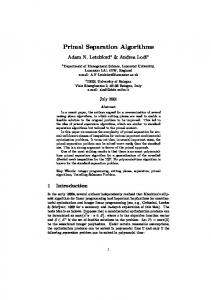
x

R1

Figure 2.2: Ghx, yi = Ghy, xi when x is reduced according to R2 . For the original valid reduction sequence, we find that Ghv1 , . . . , vr i = Ghv1 , . . . , vr−2 ihvr−1 , vr i = Ghv1 , . . . , vr−2 ihvr , vr−1 i = Ghv1 , . . . , vr−2 , vr ihvr−1 i. This shows that (v1 , . . . , vr−2 , vr , vr−1 ) is valid for G, and (v1 , . . . , vr−2 , vr ) is valid for G as well because it is a prefix. By induction, we know that (vr , v1 , . . . , vr−2 ) is valid for G, too, and Ghv1 , . . . , vr−2 , vr i = Ghvr , v1 , . . . , vr−2 i. In conclusion, we obtain Ghv1 , . . . , vr i = Ghv1 , . . . , vr−2 ihvr−1 , vr i = Ghv1 , . . . , vr−2 ihvr , vr−1 i = Ghv1 , . . . , vr−2 , vr ihvr−1 i = Ghvr , v1 , . . . , vr−2 ihvr−1 i = Ghvr , v1 , . . . , vr−2 , vr−1 i. 

15

2 MaxCut and Max2SAT Lemma 2.5 Let G = (V, E) be a graph, let D ⊆ V , and let (v1 , . . . , vr ) as well as (vπ(1) , . . . , vπ(r) ) be two valid reduction sequences for G, where π ∈ Sr is some permutation. Then Ghv1 , . . . , vr i = Ghvπ(1) , . . . , vπ(r) i. Proof. Again, the claim is obvious for r ≤ 1 and given by Lemma 2.3 for r = 2. We show the cases r > 2 by induction on r. If π(1) = 1 we can apply the induction hypothesis directly to see that Ghv1 , . . . , vr i = Ghv1 ihv2 , . . . , vr i = Ghv1 ihvπ(2) , . . . , vπ(r) i = Ghvπ(1) , . . . , vπ(r) i. Otherwise, let σ denote the sequence obtained from (vπ(1) , . . . , vπ(r) ) by removing v1 . Lemma 2.4 guarantees that Ghvπ(1) , . . . , vπ(r) i = Ghv1 ihσi. By induction, we obtain Ghv1 , . . . , vr i = Ghv1 ihv2 , . . . , vr i = Ghv1 ihσi = Ghvπ(1) , . . . , vπ(r) i.  Lemma 2.6 Let G = (V, E) be a graph, let D ⊆ V , and let (u1 , . . . , ur ) as well as (v1 , . . . , vs ) be two valid reduction sequences for G such that {u1 , . . . , ur } and {v1 , . . . , vs } are disjoint. Then (u1 , . . . , ur , v1 , . . . , vs ) and (v1 , . . . , vs , u1 , . . . , ur ) are both valid reduction sequences for G as well. Proof. Note that for any reducible w ∈ V , the reduced graph Ghwi still contains all nodes from G with the sole exception of w. Consequently, Ghu1 , . . . , ur i still contains v1 , . . . , vs . Note also that the degree of all nodes in Ghwi is smaller or the same as in G, implying that v1 is reducible in Ghu1 , . . . , ur i. Due to these facts, (u1 , . . . , ur , v1 ) is a valid reduction sequence for G. Since v2 is reducible in Ghv1 i and Ghu1 , . . . , ur , v1 i = Ghv1 , u1 , . . . , ur i according to Lemma 2.5, we know that v2 is also reducible in Ghu1, . . . , ur , v1 i. In particular, (v2 ) is a valid reduction sequence for Ghu1 , . . . , ur , v1 i and (u1 , . . . , ur , v1 , v2 ) a valid reduction sequence for G. Continuing inductively we can see that (u1, . . . , ur , v1 , . . . , vs ) is a valid reduction sequence for G. Analogously, this statement holds for the reduction sequence (v1 , . . . , vs , u1 , . . . , ur ). 

16

2.2 A Confluent Set of Reduction Rules Lemma 2.7 Let G = (V, E) be a graph, let D ⊆ V , and let σ1 τ1 , σ2 τ2 be two valid reduction sequences for G. Furthermore, assume that σ1 ∩ σ2 τ2 = ∅ and σ2 ∩ σ1 τ1 = ∅. Then there are sequences µ1 and µ2 such that σ1 τ1 σ2 µ1 and σ2 τ2 σ1 µ2 are valid reduction sequences for G with Ghσ1 τ1 σ2 µ1 i = Ghσ2 τ2 σ1 µ2 i. Proof. We use induction on |σ1 τ1 | + |σ2 τ2 |. The claim follows immediately for |σ1 τ1 | = 0 as well as for |σ2 τ2 | = 0. Let us first assume that |σ1 | + |σ2 | > 0. Since σ1 and σ2 are disjoint, Lemma 2.6 implies that σ1 σ2 and σ2 σ1 are valid reduction sequences for G. Lemma 2.5 then implies that Ghσ1 σ2 i = Ghσ2 σ1 i. (2.1) We now know that σ2 τ2 and σ2 σ1 are both valid reduction sequences for G. Hence, τ2 and σ1 are valid reduction sequences for Ghσ2 i. Furthermore, they are disjoint. Again, Lemma 2.6 and 2.5 imply that σ1 τ2 and τ2 σ1 are valid reduction sequences for Ghσ2 i and that Ghσ2 ihσ1 τ2 i = Ghσ2 ihτ2 σ1 i. In the same way we get Ghσ1 ihσ2 τ1 i = Ghσ1 ihτ1 σ2 i. We can rewrite these two equalities as Ghσ2 σ1 τ2 i = Ghσ2 τ2 σ1 i, Ghσ1 σ2 τ1 i = Ghσ1 τ1 σ2 i.

(2.2) (2.3)

Let G′ = Ghσ1 σ2 i, σ1′ = σ2′ = ε, τ1′ = τ1 , and τ2′ = τ2 . Note that σ1′ τ1′ and σ2′ τ2′ are both valid for G′ due to (2.2) and (2.3). Of course, σ1′ ∩σ2′ τ2′ = σ2′ ∩σ1′ τ1′ = ∅ because σ1′ and σ2′ are empty. Therefore, all preconditions of the lemma are fulfilled, and |σ1′ τ1′ | + |σ2′ τ2′ | < |σ1 τ1 | + |σ2 τ2 |. We can thus use the induction hypothesis to show the existence of µ′1 and µ′2 such that τ1′ µ′1 and τ2′ µ′2 are valid reduction sequences for G′ and that G′ hτ1′ µ′1 i = G′ hτ2′ µ′2 i. If we choose µ1 = µ′1 and µ2 = µ′2 , then this is exactly the same as Ghσ1 σ2 τ1 µ1 i = Ghσ1 σ2 τ2 µ2 i.

(2.4)

Using all of above we obtain (2.3)

(2.4)

Ghσ1 τ1 σ2 µ1 i = Ghσ1 σ2 τ1 µ1 i =

(2.1)

(2.2)

Ghσ1 σ2 τ2 µ2 i = Ghσ2 σ1 τ2 µ2 i = Ghσ2 τ2 σ1 µ2 i. See Figure 2.3 for an illustration. The other case is that σ1 = σ2 = ε. If τ1 = ε as well, the statement of the lemma holds because setting µ1 = τ2 and µ2 = ε guarantees that σ1 τ1 σ2 µ1 = σ2 τ2 σ1 µ2

17

2 MaxCut and Max2SAT G

σ1 Ghσ1 i

σ2 Ghσ2 i

Ghσ1 σ2 i

σ2

σ1

τ1

τ2 τ1

Ghσ1 τ1 i

τ2

σ2 Ghσ1 τ1 σ2 i

Ghσ2 τ2 i σ1 Ghσ2 τ2 σ1 i

µ1

µ2

Ghσ1 τ1 σ2 µ1 i = Ghσ2 τ2 σ1 µ2 i

Figure 2.3: Confluent sequences. and thus Ghσ1 τ1 σ2 µ1 i = Ghσ2 τ2 σ1 µ2 i. Otherwise, if τ1 is not empty, we may furthermore assume that the first vertex in τ1 also occurs in τ2 : if it did not, we could shift the first node of τ1 into σ1 and apply the argument from the above first case. Now define τ1 = vτ1′ and τ2 = τ2′ vτ2′′ . Applying Lemma 2.4 to τ2′ v yields Ghτ2′ vi = Ghvτ2′ i. This entails Ghvτ2′ τ2′′ i = Ghτ2 i. Furthermore, both τ1′ and τ2′ τ2′′ are valid reduction sequences for Ghvi. Owing to the induction hypothesis with respect to Ghvi and the sequences below, there are µ1 and µ2 such that i.h.

Ghτ1 µ1 i = Ghvihτ1′ µ1 i = Ghvihτ2′ τ2′′ µ2 i = Ghτ2 µ2 i, which completes the proof.  Theorem 2.8 Let G = (V, E) be a graph and let D ⊆ V . Then R∗ (G) is welldefined, i.e., if τ1 and τ2 are two valid reduction sequences for G of maximal length, then Ghτ1 i = Ghτ2 i. Proof. Let σ1 = σ2 = ε, then G, D, σ1 τ1 , and σ2 τ2 satisfy the conditions of Lemma 2.7. Thus there are sequences µ1 and µ2 such that σ1 τ1 σ2 µ1 = τ1 µ1 and σ2 τ2 σ1 µ2 = τ2 µ2 are valid reduction sequences for G with Ghτ1 µ1 i = Ghτ2 µ2 i. The fact that τ1 µ1 is a valid reduction sequence for G and that τ1 is a reduction sequence of maximal length implies µ1 = ε. Using the same argument, we obtain µ2 = ε. Hence, Ghτ1 i = Ghτ2 i. 

18

2.3 Bounds on Treewidth and Pathwidth

2.3 Bounds on Treewidth and Pathwidth Having established the confluence of our reduction rules, we now continue by investigating their influence on the pathwidth of graphs. The following lemmata reveal two important properties: graphs of treewidth at most two, i.e., seriesparallel graphs, collapse upon application of the reduction rules, whereas the rules R0 , R1 , and R2 can be applied without changing the treewidth of the graph, unless its treewidth is already at most two. Lemma 2.9 (see, e.g., Bodlaender [17]) Let G = (V, E) be a graph and let D = ∅. Then tw(G) ≤ 2. if and only if R∗ (G) is empty. Lemma 2.10 Let G = (V, E) be a connected graph with tw(G) > 2, and let G′ be a graph obtained from G by applying R0 , R1 , or R2 . Then tw(G) = tw(G′ ). Proof. Let T ′ be a tree decomposition for G′ . We will construct a tree decomposition T for G by modifying T ′ depending on which reduction rule was applied. Let G′ = Ghvi for some v ∈ V . Let us first investigate the case that R0 or R1 was applied to turn G into G′ . In both cases, v was removed from G. If v is an isolated node in G, we can simply add the new bag {v} to T ′ and connect it to an arbitrary bag. If v is a node of degree one in G with neighbor w ∈ N(v), it suffices to find a bag B in T ′ with w ∈ B and attach a new bag B ′ = {v, w} to B. Note that such a bag must exist in T ′ , since w ∈ V (G′ ). Otherwise, R2 was applied. Let N(v) = {w1 , w2} in G. It is sufficient to find a bag B in T ′ with w1 , w2 ∈ B and attach a new bag B ′ = {v, w1 , w2} to B. Again, such a bag must exist, since {w1 , w2} is an edge in G′ . In either case, the resulting tree T of bags is a tree decomposition for G. Moreover, we only added a bag B ′ of size at most three. If tw(G′ ) ≤ 2, then tw(G) ≤ 2, which contradicts the assumption tw(G) ≥ 3 from the statement of this lemma. Otherwise, we have tw(G′ ) ≥ 3 and tw(G′ ) = tw(G) because the old tree decomposition already contains a bag at least as large as B ′ .  Note that the construction used in Lemma 2.10 does not yield a path decomposition but only a tree decomposition. While we can modify the proof to yield a path decomposition, applying R0 , R1 , or R2 can then increase the width of a path decomposition by one in each step. However, it is possible to overcome this problem by a more sophisticated approach. Lemma 2.11 Let G = (V, E) be a graph such that R∗ (G) = ∅ where D = ∅. Then pw(G) ≤ 3 log(|V |) + 3.

19

2 MaxCut and Max2SAT Proof. Lemma 2.9 implies tw(G) ≤ 2, thus there is a separator U of size three such that all components of G\U have a size of at most (n−2)/2 [18]. If 1 ≤ |V | ≤ 3, the path decomposition consisting of exactly one bag is of size at most 3 log(|V |) + 3. Otherwise, let G \ U consist of the connected components C1 , . . . , Ck wit corresponding path decompositions P1 , . . . , Pk . We construct a path decomposition P for G by adding all nodes in U to each bag in each Pi and concatenate the resulting Pi as a path in an arbitrary order. The width of P is at most 3 log(|V |/2) + 6 ≤ 3 log(|V |) + 3.  This lemma will allow us to bound the pathwidth of graphs by modifying a small tree decomposition. Our first algorithm will compute a tree decomposition of size m/5.769 + O(log n) by removing nodes and applying the reduction rules in each step. Then, we will modify this approach by removing the same nodes but applying the reduction rules all at once afterwards. Since our reduction rules are confluent, both approaches yield the same (empty) graph. Lemma 2.10 ensures that removing the respective nodes but not applying R0 , R1 , and R2 yields a graph of treewidth at most two. Thus by Lemma 2.11, the width of the path decomposition will only be O(log n) larger than the tree decomposition. In order to bound the treewidth of a graph by m/5.769 + O(log n), we present a construction of tree decompositions based on the iterated removal of nodes where reduction rules are applied whenever possible. If the graph splits into several components, the construction can be performed for each of the components independently. Clearly, the removal of a node—combined with subsequent reductions—leads to a loss of edges as well. Since the number of edges that vanish upon deletion of a node is small in a few cases, but larger on average, we employ an amortized analysis using Measure & Conquer. Definition 2.12 Let G = (V, E) be a graph and let v ∈ V . We define  0    25/26 Φ(v) :=  25/13    deg(v)/2 and Φ(G) :=

P v∈V

Φ(v).

Observe that Φ(G) ≤ m.

20

if if if if

deg(v) < 3 deg(v) = 3 deg(v) = 4 deg(v) ≥ 5

2.3 Bounds on Treewidth and Pathwidth Lemma 2.13 Let G = (V, E) be a reduced connected graph with ∆(G) ≥ 4 such that G is not five-regular. Then there is a v ∈ V with deg(v) = ∆(G) such that Φ(G) − Φ(G \ (v)) ≥ 75/13 > 5.769. Proof. If ∆(G) = 5, choose a node v of maximum degree such that N(v) contains at least one node of degree less than five. Otherwise, simply choose a node v of maximum degree. Observe that every node in G has degree at least three because G is assumed to be a reduced graph. The removal of v decreases Φ in two ways. Firstly, the deletion of v lowers the measure of G by Φ(v). Secondly, the deletion of v lowers the degree of each neighbor of v by one, leading to another loss in the measure. If such a neighbor has degree three or four, its measure decreases by 25/26, because 25/13 − 25/26 = 25/26. If its degree equals five, its measure decreases by only 5/2 −25/13 = 15/26. In all other cases, the measure of the neighbor decreases by 1/2. If deg(v) = 4, each neighbor of v has degree three or four, and the above considerations imply Φ(G) − Φ(G \ (v)) = 25/13 + 4 · 25/26 = 75/13. In the special case that deg(v) = 5, at least one neighbor of v has degree three or four as detailed above. The removal of v thus leads to Φ(G) − Φ(G \ (v)) ≥ 5/2 + 4 · 15/26 + 25/26 = 75/13. If deg(v) ≥ 6, we easily obtain Φ(G) − Φ(G \ (v)) ≥ 3 + 6 · 1/2 = 6.  Let di denote the potential of nodes of degree i. The case where deg(v) = 5, and exactly one neighbor of v is of degree three of four (which is one the worst cases in Lemma 2.13), implies that it is optimal to set d4 = 2d3 . A short computation shows that the values for di as given by Φ are indeed optimal. However, this yields a worst bound in the case of five-regular graphs. The following lemma shows that Φ decreases sufficiently large in this case as well. Lemma 2.14 Let G = (V, E) be a reduced connected graph with ∆(G) = 5. Let v ∈ V be a node with deg(v) = 5 such that R∗ (G \ {v}) contains a five-regular component C. Then Φ(C) ≤ Φ(G) − 95/13. Proof. Since G is connected, v has a neighbor of degree three. Otherwise, each component of G \ {v} would contain at least one node of degree three or four and no reduction rules could be applied. This contradicts the existence of a five-regular component in R∗ (G \ {v}). The most simple way to obtain a five-regular component is to remove a node all of whose neighbors are of degree three. After the removal all neighbors are contracted by R2 , leading to a possibly five-regular component. Regardless of the structure of the resulting graph, the measure Φ(G) decreases by at least 5/2+5·25/26 = 95/13.

21

2 MaxCut and Max2SAT In any other case resulting in a five-regular component, the removal of v decreases the degree of some of its neighbors to three or four. In order to obtain a fiveregular component, these neighbors must either be part of a different component or must be reduced by some further reduction rules. Let ni denote the number of nodes in N(v) with degree i. Then, removing v decreases the measure of G by only 5/2 + n3 · 25/26 + n4 · (25/13 − 25/26) + n5 · (5/2 − 25/13) but the measure of C can be bounded by Φ(G) − 5/2 − n3 · 25/26 − n4 · 25/13 − n5 · 5/2. Therefore, Φ(C) is at most Φ(G) − 95/13.  Lemma 2.15 (Fomin and Høie [59]) Let G = (V, E) be a graph of maximum degree three. Then pw(G) ≤ (1 + ε)|V |/6 + log(|V |). The above lemmata already enable us to bound the treewidth of graphs in terms of m: Theorem 2.16 Let G = (V, E) be a graph. Then tw(G) ≤ |E|/5.769 + O(log n), and a respective tree decomposition can be computed in polynomial time. Proof. Without loss of generality, assume that G is connected. We prove the claim constructively by presenting Algorithm 1 that outputs the respective tree decomposition. Basically, the algorithm is really simple: it keeps on removing nodes of maximum degree and adds them to each bag of the tree decomposition. After each node removal, the aforementioned reduction rules are applied immediately. As soon as the graph becomes cubic, we obtain the rest of the tree decomposition using Lemma 2.15 The proof requires us to deal with some technicalities in order to obtain the desired result. Firstly, the removal of a node may split the graph into several components, but these can be handled independently. Secondly, we avoid removing a degree-five node with only degree-five neighbors whenever possible; this is a critical case in the analysis. To see how the algorithm can be employed to construct a tree decomposition, let G = (V, E) denote the currently inspected graph and v the node selected for removal. If G′ = G \ {v} is connected, a tree decomposition for G can be obtained by adding v to each bag of a tree decomposition for G′ . In particular, this operation cannot invalidate the tree decomposition. Otherwise, if G′ consists of several components, a tree decomposition for G can be obtained as follows: after adding v to each bag in the tree decompositions of the components, connect a new

22

2.3 Bounds on Treewidth and Pathwidth bag {v} to an arbitrary bag of every such decomposition. Again, it is easy to verify that the resulting tree of bags is a tree decomposition. As detailed in Lemma 2.9 and Lemma 2.10, the reduction rules do not increase Φ(G). Moreover, as described in the proof of Lemma 2.10, the tree decomposition can be updated accordingly whenever a reduction rule has been applied. It only remains to show that the size of the bags does not exceed the claimed bound, which is done using an amortized analysis using Φ. We distinguish three phases. As long as the graph contains nodes of degree at least six, we are in the first phase. While the maximum degree equals five or four, we are in the second phase. The third phase begins as soon as the maximum degree decreases to three or less. Observe that the maximum degree, as well as the degree of every node in the graph, decreases monotonically as we proceed to remove nodes, implying that the phases are traversed in the given order. Within the first phase, each step decreases the measure by at least 3 + 6 · 1/2 = 6: a node of degree at least six has a measure of at least 3, and each of its neighbors loses an edge, which decreases the measure by at least 1/2 per neighbor. Whenever the removed node disconnects the graph, it suffices to compute the tree decomposition for each of the respective components independently. At any point, we may thus restrict our analysis to the component having the largest measure. For the second phase, it hence suffices to analyze the cases in which the graph is connected and has maximum degree four or five. According to Lemma 2.13, each step in the second phase decreases Φ by at least 75/13 unless the graph is five-regular. When removing a node from a five-regular graph, Φ decreases by only 5/2 + 5 · (5/2 − 25/13) = 70/13. However, Lemma 2.14 implies that in the step before Φ has been decreased by at least 95/13, except for the very first step of this phase, whose constant additional cost is hidden in the O(log n) term. Thus, the average loss is 165/26 > 75/13. As soon as we enter the third phase, the remaining graph G′ = (V ′ , E ′ ) is either three-regular or empty (because a graph cannot contain nodes of degree at most two after applying the reduction rules). It obviously suffices to consider the threeregular case, in which |V ′ | = Φ(G′ ) · 26/25. By Lemma 2.15, the pathwidth of an n-node cubic graph is bounded by (1 + ε)n/6 + O(log n), where ε > 0 is an arbitrarily small constant. This implies a bound of (1 + ε)(Φ(G′ ) · 13/75) + O(log Φ(G′ )) ≤ Φ(G′ )/5.769 + O(log |V ′ |) on the treewidth of G′ . A respective tree decomposition can be computed in polynomial time [59]. 

23

2 MaxCut and Max2SAT Algorithm 1 This algorithm computes a tree decomposition. If G is five-regular then every node is preferable. Otherwise, every node of maximum degree is preferable unless it has exactly five neighbors all of which have degree five. Input: A reduced graph G Output: A tree decomposition T (G) for G 01: 02: 03: 04: 05: 06: 07: 08: 09: 10: 11: 12:

B := ∅; if G has maximum degree at most three then return path decomposition as computed by Fomin and Høie; if G consists of several independent components G1 , . . . , Gl then connect B to one bag from each T (Gi ); return this tree decomposition; else choose a preferable node v; G′ = G \ {v}; T ′ = T (R∗ (G′ )); Update T ′ according to every applied reduction rule; Add v to each bag of T ′ ; return T ′ ;

It now remains to show how Algorithm 1 can be modified to output a path decomposition. First, we need the following technical lemma. Lemma 2.17 Let G be a graph, let D = ∅, and let (V ′ , E ′ ) = R∗ (G). Then every connected component of G[V \ V ′ ] is connected to at most two vertices in G[V ′ ]. Proof. Let C = G[{v1 , . . . , vr }] be a connected component of G[V \ V ′ ]. G has been reduced to (V ′ , E ′ ) by a valid reduction sequence σ. Observe that σ contains v1 , . . . , vr — without loss of generality in this order. Moreover, v1 is reducible in G, because no neighbor of v1 is removed before v1 . Lemma 2.4 shows that we can move v1 to the front of σ. Repeating this argument inductively, we see that (v1 , . . . , vr ) is a valid reduction sequence for G. Moreover, applying any reduction rule on C does not affect the connectivity of the remaining nodes in C, since only nodes of degree one or less are removed and nodes of degree two are contracted. Let

Vi := { v ∈ V ′ | v is a neighbor of {vi , . . . , vr } in Ghv1 , . . . , vi−1 i }.

We claim Vi = Vi+1 for 1 ≤ i ≤ r − 1. If vi has no neighbor in Vi (in the graph Ghv1 , . . . , vi−1 i), the claim obviously holds. Otherwise, vi is of degree two with neighbors u ∈ V ′ and w ∈ {vi+1 , . . . , vr }. Vi \ {u} ⊆ Vi+1 , as all these nodes have neighbors in {vi+1 , . . . , vr }.

24

2.3 Bounds on Treewidth and Pathwidth Applying R2 on vi adds a new edge between u and w. Since w ∈ Ghv1 , . . . , vi i, u ∈ Vi+1 . Thus V1 = Vr . Now, if |Vr | ≥ 3, then vr is not reducible in Ghv1 , . . . , vr−1 i, a contradiction.  Theorem 2.18 Let G = (V, E) be a graph. Then pw(G) ≤ |E|/5.769 + O(log n), and a respective path decomposition can be obtained in polynomial time. Proof. Let D be the set of nodes that have been chosen as preferable nodes in line (7) of Algorithm 1. The algorithm transforms G into a cubic graph Ghσi, where σ is a valid reduction sequence with respect to D. Note that every node in D is reducible in G. By Lemma 2.4 there is a valid reduction sequence σ ′ = (d1 , . . . , dr , v1 , . . . , vs ) that is a permutation of σ and di ∈ D, vi ∈ / D. Moreover, Ghσi = Ghσ ′ i. We will modify Algorithm 1 so as to construct a path decomposition instead of a tree decomposition. Without loss of generality, we assume Ghσ ′ i is connected. Otherwise, we apply the following argument for each component separately. Let P = (P1 , . . . , Pt ) be a path decomposition for Ghσ ′ i as computed by Fomin and Høie. A component C of G[{v1 , . . . , vs }] has at most two neighbors in Ghσ ′ i according to Lemma 2.17. If there are indeed two neighbors they must be connected by an edge in Ghσ ′ i as the path connecting both neighbors in C has been contracted to a single edge. Thus the neighbors occur together in a bag of P . Let Pi be the smallest bag in P that contains all neighbors of C and P ′ = (P1′ , . . . , Pk′ ) be a path decomposition of C. Since C is series-parallel, the width of P ′ is only O(log n). Then (P1′ ∪ Pi , . . . , Pk′ ∪ Pi ) is a path decomposition for G[V (C) ∪ Pi ] and (P1 , . . . , Pi , P1′ ∪ Pi , . . . , Pk′ ∪ Pi , Pi+1 , . . . Pt ) a path decomposition for G[U] where U consists of all nodes in C and Ghσ ′ i. Notice that we can do this for all components of G[{v1 , . . . , vs }] in parallel, such that the size of the resulting bags is still bounded by the width of P plus O(log n), since the original bags from P remain untouched and thus can be used as smallest bag Pi . Therefore, we obtain path decompositions for every maximal connected component of Ghd1 , . . . , dr i. In order to obtain path decompositions for each connected component of Ghd1, . . . , dr−1 i, we proceed as follows: We add dr to every bag of the path decomposition of each connected component that is adjacent to dr — just as in Algorithm 1. Afterwards, we connect these path decompositions as a path. Compared to the tree decompositions described in Theorem 2.16 only the incorporation of the path decompositions of G[{v1 , . . . , vs }] increases the size of the bags as described above. We obtain a bound of O(log n) + |E|/5.769 + O(log n) = |E|/5.769 + O(log n)

25

2 MaxCut and Max2SAT for the width of our path decomposition.  Employing a framework for algorithms that work on tree decompositions by Telle and Proskurowski [123], one immediately obtains the following result: Corollary 2.19 Max-2SAT and Max-Cut can be solved in O ∗ (2m/5.769 ) using exponential space. The exponential space complexity of the resulting algorithms is due to dynamic programming on the actual tree decomposition. As we will see in the next section, tree decompositions that were computed according to Theorem 2.16 have a unique structure: instead of adding nodes to the tree decomposition when they are removed from the graph in the first two phases and solving the problem at hand with the framework by Telle and Proskurowski, we can simply branch on these nodes if there are appropriate reduction rules for that problem. Since branching requires only polynomial space, this will enable us to get rid of the exponential space complexity. Unfortunately, the algorithm by Fomin and Høie employed in the third phase does not necessarily output decompositions of the aforementioned structure. Since this forbids us to switch to algorithms that branch directly, the third phase forces us to use the Telle–Proskurowski approach—and thus cannot be considered intuitive.

2.4 A General Framework for Intuitive Algorithms In order to obtain a framework to develop intuitive algorithms, we now abandon the special processing of cubic graphs as well as the dynamic programming. The resulting algorithms solely rely on branching and guarantee polynomial space complexity at the expense of slightly worse runtime bounds. However, this branching is only possible for problems that can be represented as graph problems with appropriate reduction rules for nodes of degree at most two. In contrast to previous algorithms [10, 66, 102] for Max-Cut and Max-2SAT, our framework (see Algorithm 2) consists of only few reduction rules and a straightforward branching rule. In the case of Max-2SAT for example, a variable x that occurs with at most two other variables y, z, we can eliminate x by adding new clauses over y and z. If branching leads to several independent subformulas, we can solve these independently—a very natural reduction. Finally, the algorithm simply branches by setting a variable x to true or false, which is probably the most simple branching possible.

26

2.4 A General Framework for Intuitive Algorithms Since we cannot rely on the result for cubic graphs by Fomin and Høie [59] any longer, we need to redefine the node measures. The following values turn out to be the best choice for our analysis. Definition 2.20 Let G = (V, E) be a graph and let v ∈ V . We define  0    30/23 Ψ(v) :=  45/23    deg(v)/2 and Ψ(G) :=

P v∈V

if if if if

deg(v) < 3 deg(v) = 3 deg(v) = 4 deg(v) ≥ 5

Ψ(v).

As in Definition 2.12, the measure of any graph is bounded by its number of edges. Lemma 2.21 Let G = (V, E) be a reduced, connected graph with ∆(G) = 4 . Let v ∈ V be a node with deg(v) = 4 such that R∗ (G \ {v}) contains a four-regular component C. Then Ψ(C) ≤ Ψ(G) − 165/23. Proof. This is can be proven analogously to Lemma 2.14. Since G is connected, v has a neighbor of degree three. Otherwise, each component of G \ {v} would contain at least one node of degree three or four and no reduction rules could be applied. This contradicts the existence of a four-regular component in R∗ (G\{v}). The most simple way to obtain a four-regular component is to remove a node all of whose neighbors are of degree three. After the removal all neighbors are contracted by R2 , leading to a possibly four-regular component. Regardless of the structure of the resulting graph, the measure Ψ(G) decreases by at least 45/23 + 4 · 30/23 = 165/23. In any other case resulting in a four-regular component, the removal of v decreases the degree of some of its neighbors to three. In order to obtain a four-regular component, these neighbors must either be part of a different component or must be reduced by some further reduction rules. Let ni denote the number of nodes in N(v) with degree i. Then, on removal of v the measure of G decreases by only 45/23 + n3 · 30/23 + n4 · (45/23 − 30/23) ≥ 105/23 but the measure of C can be bounded by Ψ(G) − 45/23 − n3 · 30/23 − n4 · 45/23. Therefore, Φ(C) is at most Ψ(G) − 165/13. 

27

2 MaxCut and Max2SAT Lemma 2.22 Let G = (V, E) be a graph such that R∗ (G) is not empty. If R∗ (G) consists of multiple components, then each component has a measure of at most Ψ(G) − 120/23. Proof. Each component of R∗ (G) contains a node v of degree at least three. The neighbors of v have degree at least three as well. Hence, the measure of each component is at least 4 · 30/23. If there are multiple components, the measure of each is thus bounded by Ψ(G) − 120/23.  Using the above two lemmata, it is possible to find small node sets that either split a graph into several components of bounded Ψ or leave a trivial graph. This is formalized by the following theorem which is the backbone of our framework. Theorem 2.23 Let G = (V, E) be a graph. There is a set D ⊆ V such that either • R∗ (G \ D) contains at least two components, each having a measure of at most Ψ(G) − 5.217|D|, or • R∗ (G \ D) = ∅ and |D| ≤ Ψ(G)/5.217 + 1. Proof. Let G = (V, E) be a graph. If G has maximum degree at least five, removing a node of maximum degree and applying the reduction rules decreases the measure by at least 2.5 + 5 · (2.5 − 45/23) = 120/23 > 5.217. We may thus assume that G has maximum degree at most four. Analogously to Theorem 2.16, we remove nodes of maximum degree until G either splits into several components or becomes empty. In doing so, we avoid nodes with four neighbors of degree four if possible. Again, the measure decreases by at least 120/23 in any step, except for the aforementioned four-regular case. But even in this case with a loss of 45/23 + 4 · 15/23 = 105/23, there is an average loss of more than 120/23 according to Lemma 2.21, since the step before yields a loss of at least 165/23. There is only one exception that does not allow for the above bonus argument, namely the case when the input graph is four-regular for the first time. Note that the loss of measure in this case only amounts to 105/23, which is 15/23 short of the desired value. If we end up with an empty graph, the additional node in D is absorbed by the last summand in the bound Ψ(G)/5.217 + 1. Otherwise, if the graph breaks down into several components, the remaining measure is at most Ψ(G) − 5.217|D| + 15/23. Lemma 2.22 implies that each component has measure at most Ψ(G) − 5.217|D| + 15/23 − 120/23 < Ψ(G) − 5.217|D|. Note that according to our results from Section 2.2, reducing the graph G\D yields exactly the same graph as removing the nodes in D successively and reducing the

28

2.4 A General Framework for Intuitive Algorithms remaining graph in each step. Hence, the nodes selected by the above algorithm constitute a set D with the desired properties.  Note that similar to the proofs from Section 2.3, this result can be used to bound the pathwidth of sparse graphs by m/5.127+3. While this bound is worse than the one obtained earlier, the corresponding path decompositions have nice properties that can be exploited in direct, intuitive algorithms as we will see shortly. Definition 2.24 Let L be a language over the alphabet Σ, let G be the family of all graphs and let ϕ : Σ∗ → G be a mapping that can be computed in polynomial time. Then ϕ is a graph representation of L. Definition 2.25 Let I ∈ Σ∗ be an instance of some problem with graph representation ϕ. We define the splitting number s(I) of a run of Algorithm 2 on I as: • s(I) := 0 if the algorithm returns in line (2) . • s(I) := 1 + max{ s(Ii) | i = 1, . . . , l } if the algorithm returns in line (4). • s(I) := s(I1 ) if the algorithm returns in line (7). Algorithm 2 A simple algorithm that decides membership in L. See Theorem 2.26 for a description of the notation used here. Input: I ∈ Σ∗ Output: ρ(I)= true, if I ∈ L. 01: 02: 03: 04: 05: 06: 07:

Compute I ′ = f (I) and ϕ(I ′ ); if tw(ϕ(I ′ )) ≤ 2 then solve I ′ ∈ L in polynomial time; if ϕ(I ′ ) consists of components G1 , . . . , Gl with corresponding I1 , . . . , Il (3) then solve I ′ ∈ L by testing Ii ∈ L for all 1 ≤ i ≤ l; else pick a v ∈ ϕ(I ′ ) and compute corresponding I1 , . . . , Ik (4); solve I ′ ∈ L by testing Ii ∈ L for all 1 ≤ i ≤ k

Theorem 2.26 Let L be a language over the alphabet Σ with graph representation ϕ and let k ∈ N. Moreover, let t : Σ∗ → N such that the following conditions hold for all I ∈ Σ∗ . 1. I ∈ L can be tested in time O(t(I)) if tw(ϕ(I)) ≤ 2. 2. There is a mapping f such that f (I) ∈ L ⇔ I ∈ L, f (f (I)) = f (I) and R∗ (ϕ(I)) = ϕ(f (I)) and f can be computed in time O(t(I)).

29

2 MaxCut and Max2SAT 3. If ϕ(I) consists of several components G1 , . . . Gl , it is possible to compute I1 , . . . , Il in time O(t(I)) such that: • ϕ(Ii ) = Gi for all 1 ≤ i ≤ l • and I ∈ L can be decided in time O(t(I)) if membership in L is known for all Ii . 4. For any v ∈ V (ϕ(I)), there are instances I1 , . . . , Ik computable in O(t(I)) such that • ϕ(Ii ) = ϕ(I) \ {v} for all 1 ≤ i ≤ k • I ∈ L can be decided in time O(t(I)) whenever membership in L for I1 , . . . , Ik is known. Then I ∈ L can be decided in time O(k |E(ϕ(I)|/5.217 (t(I)) by Algorithm 2. Proof. Let ϕ(f (I)) = G and Ψ(I) = Ψ(G). Let D = {v1 , . . . , v|D| } ∈ V (G) be the set of nodes given by Theorem 2.23 and let I r denote the set of instances computed from I by Algorithm 2 in r recursive steps and after applying the reduction rules f in Line 1 (and thus I 0 = {f (I)}). Moreover, let s denote the smallest number such that I s contains an instance I ′ such that either ϕ(I ′ ) consists of several components or tw(I ′ ) ≤ 2. We easily obtain ϕ(I1 ) = ϕ(I2 ) with I1 , I2 ∈ I r for any 1 ≤ r ≤ s as follows. Let I ′ be an instance in I r−1 . We have ϕ(Ii ) = ϕ(f (Ii′ )) (for i ∈ {1, 2}) where Ii′ is an instance used in the recursive call in Line 7. By Condition (2) we have ϕ(Ii ) = R∗ (ϕ(Ii′ )) and by Condition (4) ϕ(Ii′) = ϕ(I ′ ) \ {v}. Thus, we obtain ϕ(I1 ) = R∗ (ϕ(I1′ )) = R∗ (ϕ(I ′ ) \ {v}) = R∗ (ϕ(I2′ )) = ϕ(I2 ) This allows us to use the well-defined notation ϕ(I t ) := ϕ(I ′ ) for any I ′ ∈ I t . Before we can proof the runtime bound of the theorem, we need to show that R∗ (G\D) = ϕ(I |D| ). We prove the stronger statement R∗ (G\{v1 , . . . , vt }) = ϕ(I t ) by induction. For the base step where t = 0, this holds because I 0 = {f (I)} and thus R∗ (ϕ(G)) = ϕ(f (I)) = ϕ(G). For the induction step, R∗ (G \ {v1 , . . . , vt }) = R∗ (R∗ (G \ {v1 , . . . , vt−1 }) \ {vt }) holds because R∗ is confluent and R∗ (R∗ (G \ {v1 , . . . , vt−1 }) \ {vt }) = R∗ (ϕ(I t−1 ) \ {vt }) = ϕ(I t ), follows by induction. Hence, we also obtain s = |D|. We are now able to bound the number of leaves in the recursion tree of Algorithm 2 by |G|2Ψ(G)/5.217 using induction over the splitting number s(I). If s(I) = 0, Line 4 is never executed. Thus, tw(ϕ(I s )) ≤ 2. Theorem 2.23 implies s = |D| ≤

30

2.4 A General Framework for Intuitive Algorithms Ψ(G)/5.217 and thus the depth of the recursion is bounded by Ψ(ϕ(I))/5.217. Since we need to compute k recursive calls, we can bound the number of leaves in the recursion tree by |G|k Ψ(G)|/5.217 , i.e., |I s | ≤ k Ψ(G)/5.217 . If s(I) > 0, ϕ(I s ) decomposes into several components G1 , . . . , Gl . For each I ′ ∈ I s , we thus need to compute the solution for l smaller instances I1 , . . . , Il (according to Condition (3)). By Theorem 2.23, the measure of each Ψ(Gi ) is bounded by Ψ(G)−s·5.217 and similar to above, we have |I s | ≤ k Ψ(G)/5.217 . Using the induction hypothesis, we bound the number of recursive calls by ks ·

l X

|Gi| · k (Ψ(G)−s·5.217)/5.217

i=1 s

= k ·k

(Ψ(G)−s·5.217)/5.217

·

l X

|Gi| = |G| · k Ψ(G)/5.217 .

i=1

Since the number of leaves in the recursion tree is bounded by |G| · k Ψ(G)/5.217 and each call takes only O(t(I)), the running time of Algorithm 2 is O(k t/5.217 t(I)).  We can thus solve any problem with our framework as long as 1. small instances, i.e., instances whose graph representation are of treewidth at most two, can be solved in polynomial time, 2. there are reduction rules that carry over to R on the graph representation, 3. the problem decomposes into independent subinstances whenever the graph representation consists of several connected components, and 4. there is branching rule that corresponds to removing a single node from the graph representation.

2.4.1 Algorithms for Max-2SAT and Max-Cut In order to obtain intuitive algorithms for Max-Cut and Max-2SAT, it now remains to find such operations 1, 2, 3, and 4. When F is a Max-2SAT formula, we use GF to denote the connectivity graph of F : each variable in F is represented by a node in GF , and two nodes are connected if and only if the formula contains a clause consisting of the two corresponding variables. Observe that the connectivity graph does not represent negations or weights in the formula. For instance, f = (x1 ∨ x2 ) ∧ (x1 ∨ x2 ) ∧ (x2 ∨ x3 ) and g = (x1 ∨ x2 ) ∧ (x2 ∨ x3 ) have identical connectivity graphs Gf and Gg . As a consequence, the formula F cannot be reconstructed from GF .

31

2 MaxCut and Max2SAT In order to fix a terminology for the discussion of satisfiability problems, we adhere to the notation for weighted boolean formulas used by Gramm, Hirsch, Niedemeier, and Rossmanith [66]. Definition 2.27 A (weighted) clause is a pair (ω, S) where ω is an integer and S is a nonempty finite set of literals that does not contain, simultaneously, any variable together with its negation. A formula F is a set of clauses, such that each set of literals appears in at most one clause. We call ω the weight of a clause (ω, S) and define ( wF (S) =

ω 0

if (ω, S) ∈ F , otherwise.

In addition to usual clauses, we allow a special true clause (ω, T) which is satisfied by every assignment. (We also call it a T-clause.) The operators + and − are defined: Definition 2.28 F + G = { (wF (S) + wG (S), S) | wF (S) + wG (S) 6= 0 } F − G = { (wF (S) − wG (S), S) | wF (S) − wG (S) 6= 0 } For a literal l and a formula F , the formula F [l] is obtained by setting the value of l to T rue. For a set of literals X = {x1 , . . . , xk }, we set F [X] := F [x1 ][x2 ] . . . [xk ]. For example F = {(5, {x, y, z¯}), (3, {y, z¯}), (2, {¯ x, y}), (−1, {¯ x, y, z¯})} F [x] = {(5, T), (2, {y, z¯}), (2, {y})} F [¯ x] = {(1, T), (8, {y, z¯})} F [x, y] = {(9, T)}. Definition 2.29 The optimal value of a maximum weight assignment for formula F is defined as OptVal (F ) = maxA { ω | (ω, T) ∈ F [A] }, where A is taken over all possible assignments. An assignment A is optimal if F [A] contains only one clause (ω, T) (or does not contain any clause, in this case we set ω = 0) and OptVal (F ) = ω (= OptVal (F [A]) ). We call F and G max-equivalent if OptVal (F ) = OptVal (G).

32

2.4 A General Framework for Intuitive Algorithms In order to design a branching algorithm for Max-2SAT as suggested above, we must find reduction rules for formulas that correspond to removing nodes of degree at most one and contracting nodes of degree two. Clearly, a simple reduction rule suffices to remove nodes of degree zero from GF : If a variable only occurs in unary clauses, it is optimal to choose the assignment that satisfies the most of these clauses. Variables that occur together with at most two other variables require more complex reduction rules. In order to maintain a max-equivalent formula, these steps require us to introduce new clauses. Since we branch on nodes in the connectivity graph that hides negations it is straightforward to analyze the running time without respect to negations as well. This notion is reflected by the following definition. Definition 2.30 Let F be a SAT formula. For each clause C, we call the set of variables that occur in C the clause type. The clause types of F are the clause types of the clauses in F . For example, (x1 ∨ x2 ) and (x1 ∨ x2 ) have the same type and may thus be counted as one entity in the analysis. This way of measuring the complexity of a formula by the number of clause types has a crucial advantage: we may employ reduction rules that introduce additional clauses of existing types without raising the measure. Definition 2.31 Let F be a 2SAT formula. We call the variable x a companion (of y) if there is a unique variable y 6= x that occurs together with x in a clause. In terms of the respective connectivity graph GF , the variable x is a companion if and only if the degree of x in GF is one. Lemma 2.32 (Companion reduction rule) Let F be a 2SAT formula. If x is a companion, we can transform F into a max-equivalent formula F ′ containing the same variables except for x, where GF ′ = GF \ {x}. This can be done in polynomial time. Proof. Let F be a formula, let x be a companion of y, let F ′ consist of all clauses in F with an occurrence of the variable x, and let F ′′ = F \ F ′ . Let furthermore a = OptVal (F ′ [y]), b = OptVal (F ′ [¯ y ]), and ( (b, T), (a − b, {y}) if a > b H=  (a, T), (b − a, {¯ y }) otherwise.

33

2 MaxCut and Max2SAT It is easy to see that a = OptVal (H[y]) and b = OptVal (H[¯ y]). We immediately get OptVal (H + F ′′ ) =  max OptVal (H[y]) + OptVal(F ′′ [y]), OptVal(H[¯ y ]) + OptVal (F ′′ [¯ y ]) =  max OptVal (F ′ [y]) + OptVal (F ′′ [y]), OptVal(F ′ [¯ y ]) + OptVal(F ′′ [¯ y ]) = = OptVal (F ′ + F ′′ ) = OptVal (F ). Hence, we can replace F by the max-equivalent formula H + F ′′ . Note that it is easy to calculate a and b, and that H + F ′′ does not contain the variable x anymore.  Definition 2.33 Let F be a 2SAT formula. A variable x is a double companion if and only if the degree of x in GF is two. For the following lemma, remember the definition of our new parameter t, the number of clause types. Lemma 2.34 (Double companion reduction rule) Let F be an 2SAT formula. If x is a double companion, then we can transform F into a max-equivalent formula F ′ that contains the same variables as F except x, and possibly clauses of negative weight, in polynomial time. The formula F ′ does not have more clause types than F . Moreover, GF ′ is the graph obtained from GF by contracting x. Proof. Let x be a double companion that occurs together with y and z. Let F = F ′ + F ′′ , where F ′ consists of all the clauses that contain x and F ′′ holds all the other clauses. We define a = OptVal (F ′ [y, z]), b = OptVal (F ′ [y, z¯]), c = OptVal (F ′ [¯ y , z]), and d = OptVal (F ′ [¯ y , z¯]). Let  G = (a + b + c + d, T), (−d, {y, z}), (−c, {y, z¯}), (−b, {¯ y , z}), (−a, {¯ y , z¯}) . We easily see a = OptVal (G[y, z]), b = OptVal (G[y, z¯]), c = OptVal (G[¯ y , z]), and ′ ′′ ′′ d = OptVal (G[¯ y , z¯]). Therefore, OptVal (F + F ) = OptVal (G + F ). Moreover, x does obviously not occur in G + F ′′ . Note that the new clauses containing y and z imply the existence of an edge between the corresponding nodes in GF ′ . Hence, GF ′ can be obtained from GF by contracting x.  We now have reduction rules for formulas in 2-CNF that enable us to eliminate all nodes with degree up to two in the corresponding connectivity graph. The following lemma shows how branching on a variable affects the connectivity graph.

34

2.4 A General Framework for Intuitive Algorithms Lemma 2.35 Let F be a formula and let x be a variable. Then GF [x] = GF [x] = GF \ {x}. Proof. Let F containing x result in the {x} = GF [x] .

be a formula and x a variable. Setting x to true removes every clause and shrinks each clause containing x to size one. Both operations removal of all corresponding edges in GF . Therefore, GF [x] = GF \ 

Definition 2.36 Let F be a formula over variables x1 , . . . , xn such that GF is connected. If GF is four-regular or its maximum degree does not equal four, the preferable variable is the first xi of maximum degree. Otherwise, if GF has maximum degree four as well as nodes of smaller degree, the preferable variable is the first xi of degree four with at least one neighbor of smaller degree. Algorithm 3 A very simple algorithm for Max-2SAT that does not use the connectivity graph directly. Input: A Max-2SAT-formula F Output: OptVal (F ) 01: 02: 03: 04: 05: 06: 07:

Reduce F by the reduction rules while possible; if F = {(k, T)} then return k; if F consists of several Pl independent subformulas F1 , . . . , Fl then return i=1 OptVal (Fi ); else Let x be the preferable variable; return max{OptVal (F [x]), OptVal (F [¯ x])};

Algorithm 3 can easily be seen as a direct realization of our framework as proposed in Algorithm 2. Theorem 2.37 Let F be a formula. Using only polynomial space, Algorithm 3 solves Max-2SAT in time O(2t/5.217 |F |2 ) on F , where t is the number of clause types. Proof. The connectivity graph GF satisfies all four requirements of Theorem 2.26. 1. If tw(GF ) ≤ 2, the reduction rules reduce F to a formula consisting of only one variable. Hence, we can solve Max-2SAT with input F in polynomial time in this case. 2. As outlined above, the companion rule and the double companion rule can be used to obtain f .

35

2 MaxCut and Max2SAT 3. If GF consists of several components, the corresponding formulas are independent, i.e., consist of disjoint sets of variables. Thus, we can simply add the optimal values for each subformula to obtain an optimal solution. 4. Simply branching on a variable x yields the desired rule by Lemma 2.35. Finally, finding reducible variables can easily be done in O(|F |), whereas applying the reduction rules might need at most O(|F |) steps.  Using the well-known reduction from Max-Cut to Max-2SAT which consists of two clauses for each edge but only one clause type, we obtain the following corollary: Corollary 2.38 Let G be a graph. Max-Cut can be solved in time O(2m/5.217 m2 ) on G using only polynomial space, where m denotes the number of edges in G. It is very simple to construct reduction rules for Max-Cut to deal with nodes of degree at most two. In doing so, the construction of a direct algorithm similar to Algorithm 3 for Max-Cut is straight forward.

2.5 Implementation In this section, we present an implementation of our treewidth algorithm. Here, as well as in all following implementations, we use the LEDA library [3, 91] as underlying framework, since this allows us to use concentrate on the implementation of our algorithm while the basic graph operations are handled by LEDA. For various reasons, we present here a slightly modified version of our algorithm. While Algorithm 1 — as presented above — can easily be implemented, we here omit the use of the algorithm by Fomin and Høie for the sake of readability. Therefore, the size of obtained tree decomposition can only be bounded by m/5.217. Nevertheless, both bounds do not differ much on practical input instances, as the bound of (1 + ε)n/6 + O(log n) depends heavily on ε and the constants in the O-notation. Moreover, while a small tree decomposition for cubic graphs can be computed in polynomial time, the runtime required for this should not be considered efficient as the polynomials in the runtime bound tend to be rather large. Furthermore, Algorithm 1 is called recursively for each preferable node that is removed. Note that the algorithm has a typical recursive pattern: a node is removed from the graph, then the algorithm is called recursively and finally the tree decomposition is updated. Therefore, a recursive approach is the most simple implementation for this strategy. If we would stick to this behavior, it would be reasonable to implement the simplification routine recursive as well. Such an

36

2.5 Implementation implementation would be very simple and straightforward. Unfortunately, it would also be very slow, as the overhead caused by the recursive calls would be very large. More precisely, we would need a recursive call for each node in the graph, which can cause problems for graphs as small as a few thousand nodes. In the implementation presented here, we only use recursive calls whenever the graph splits into several components. The construction of the tree decomposition is done with the help of an additional stack, that stores which nodes and edges where removed. A big surplus of this method is that we can easily stick to references to the graph and the tree decomposition instead of copies. Since the graph is heavily modified within our algorithm, we can either undo all changes or work on a copy of the graph. Obviously, the latter is much slower while the first requires a more complex algorithm. Fortunately, LEDA allows us to hide nodes and edges temporarily from the graph, which provides a great tool for the reversal of all modifications to the graph. Listing 2.1 shows the code for the main function. void Algorithms::computeTreeDecomposition(graph &G, TreeDecomposition &tree) { removalList removed; while(G.number of nodes()>0 && isConnected(G) ){ simplify(G,tree,removed); if (G.number of nodes()>0){ node u=nodeOfMaxDegree(G); removed.push(removalItem(u,adjacentEdges(G,u))); G.hide node(u); } } if (! isConnected(G)) combineSolutions(G,tree); createDecomposition(G,tree,removed); }

Listing 2.1: An implementation of Algorithm 1. Note that the application of the simplification rules, the combination of solutions for several components, and the concluding construction of the tree decomposition are handled in separate functions. Listing 2.2 shows the implementation of the latter function, which is surprisingly simple: all we have to do is check which rule was applied (R0 , R1 , R2 or RD ), modify the tree decomposition accordingly and undo the removal of the respective node. All other methods are equally simple and very efficient as well. void Algorithms::createDecomposition(graph &G, TreeDecomposition &tree, removalList &removed) { removalItem rem;

37

2 MaxCut and Max2SAT

}

edge e; while(removed.size()>0){ // Get pair (node u, adjacent edges to u) from list rem=removed.pop(); node u=rem.first; list edges =rem.second; list neighbours; forall (e,edges) neighbours.push(target(e)); // A node of maximum degree was removed if (neighbours.size()>2) tree .addNodeToEachBag(u); // Either R0 or R1 were applied if (neighbours.size()=1){ node b = tree.findBagContaining(neighbours); neighbours.push(u); tree .addNewBagToB(neighbours,b,u); } // R0 was applied if (neighbours.size()==0){ list bag; bag.push(u); tree .addNewBag(bag); } // Undo changes to the graph G.restore node(rem. first ); forall (e, edges) if (addedEdges.search(e)==nil && addedEdges.search(G.reversal(e))==nil) G.restore edge(e ); G.make bidirected(); G.make map(); } tree .sortBags();

Listing 2.2: Building a tree decomposition from the previously stored information. Figure 2.5 shows a tree decomposition computed by our algorithm for the graph depicted in Figure 2.4. Note the special structure of the decomposition, where some nodes appear in almost all bags. The performance of our algorithm is governed by two important factors. Firstly, the decompositions should be computed in reasonable time. If the constructed decomposition will be used to solve problems for the underlying graph, the computing of the tree decomposition itself must be significantly faster than applied algorithm. Although the polynomial bound on the runtime imply that this holds

38

2.5 Implementation 43

6

12

37

35

41 10

40

16

19

32

34

28 36

2

42

29 8

30

9

11

4

46

7

31

49

50

25 17

38

21

15

33

14

45 26 5

23 13 47

3

18 22

27

44

20

48

39

1

24

Figure 2.4: A random graph with 50 nodes and 122 edges. . A corresponding tree decomposition is depicted in Figure 2.5. in theory, this is not necessarily the case in practice. For example, the famous algorithm by Bodlaender computes an optimal tree decomposition in time f (k) · n. Nevertheless, this algorithm is extremely slow even for very small k [83]. In order to obtain an estimation of the runtime of our algorithm on practical instances, we tested it on various instances. Table 2.1 shows that the runtime was indeed very reasonable even for large graphs. As tree decompositions are mostly used in exact algorithms, a far more important factor is the size of the constructed decompositions. Whenever the graph is very dense, almost every node is contained in almost all bags. This is of course not very surprising, as for dense graphs, even the tree decomposition consisting of exactly one bag satisfies a bound on the bound of m/5.769. Moreover, the treewidth of

39

2 MaxCut and Max2SAT 3, 14, 15, 17, 19, 22, 26 32, 33, 35, 42, 46, 48

3, 14, 15, 17, 19, 21 28, 32, 33, 35, 42

3, 7, 14, 15, 17, 19 21, 32, 33, 35, 42

15, 34, 41

3, 14, 15, 17, 19, 26, 28 32, 33, 35, 42, 46, 48

18, 25, 47

1, 3, 15, 17, 20 32, 35, 42, 44

3, 11, 15, 17, 19, 20, 25, 26 28, 32, 33, 35, 42, 46, 48

8, 15, 17, 32, 35 37, 41, 42

3, 10, 15, 17, 19, 32, 33 35, 42, 43, 45, 46

3, 11, 15, 17, 19, 20, 25, 26 32, 33, 35, 42, 45, 46, 48

3, 15, 17, 19, 25, 32, 33 35, 42, 44, 46, 47, 48

3, 11, 15, 17, 19, 20, 25, 32 33, 35, 42, 44, 45, 46, 48

2, 3, 8, 11, 15, 17, 19, 32 33, 35, 41, 42, 46, 48

3, 11, 15, 17, 19, 25, 26, 32 33, 35, 42, 43, 45, 46, 48

3, 8, 11, 15, 17, 19, 25, 26, 30 32, 33, 35, 42, 43, 46, 48

3, 15, 17, 27, 32 35, 42, 45, 48

2, 3, 8, 11, 15, 17, 19, 25, 26 30, 32, 33, 35, 42, 46, 48

3, 8, 11, 15, 17, 19, 25, 26, 30 32, 33, 35, 36, 42, 46, 48

3, 6, 8, 11, 15, 17, 19, 25, 30 32, 33, 35, 42, 43, 46, 48

3, 6, 8, 11, 12, 15, 17, 19 32, 33, 35, 42, 46, 48

2, 3, 11, 15, 17, 19, 31, 32 33, 35, 41, 42, 46, 48

11, 33, 49

3, 11, 13, 15, 17, 19, 25, 26, 30 32, 33, 35, 36, 42, 46, 48

3, 11, 15, 17, 19, 25, 26, 30 32, 33, 35, 42, 43, 46, 48

5, 24, 48

3, 5, 9, 11, 15, 17, 19 32, 33, 35, 42, 46, 48

3, 9, 11, 15, 17, 19, 29, 30 32, 33, 35, 42, 46, 48

3, 11, 13, 15, 17, 19, 25, 29, 30 32, 33, 35, 36, 42, 46, 48 3, 11, 15, 17, 19, 25, 30, 32 33, 35, 42, 43, 46, 48

3, 13, 15, 17, 19, 29, 32 33, 35, 38, 42, 46

3, 13, 15, 17, 23 32, 35, 38, 42

3, 4, 11, 13, 15, 17, 19, 25 32, 33, 35, 36, 42, 46, 48

3, 4, 15, 17, 19, 25, 32 33, 35, 39, 42, 46, 48

3, 15, 17, 32, 35 36, 42, 46, 50

16, 35, 36

∅ 40

Figure 2.5: A tree decomposition of width 15 = m/8.13 for the graph depicted in Figure 2.4 as computed by Algorithm 1 without applying the method by Fomin and Høie. these graphs tends to be almost the number of vertices. Therefore, we are more interested in the tree decomposition of sparse graphs. On random sparse graphs, the graph model affects the outcome largely. Using the LEDA function random simple undirected graph, we can construct graphs of a given average degree. On such graphs, the algorithm computes tree decompositions of width m/7.8 in the average. This is due to the fact that such graphs contain some nodes of very high degree and some of very low degree. For example the graph depicted in Figure 2.4 contains the node 17, which is of degree ten. Removal of such a node obviously creates a smaller graph than predicted by the analysis, as many edges are removed and the measure of many nodes is reduced as well. Moreover, all nodes of degree at most two can be reduced at the beginning. This

40

2.5 Implementation |V | |E| time (s) 500 500 0.2 500 1000 0.5 500 2000 0.8 500 3000 1.0 500 4000 1.4 500 5000 1.8 500 6000 2.0 500 50000 43.5 500 100000 107.9 500 124750 141.8 1000 3000 3.9 2000 6000 21.2 5000 15000 232.1 Table 2.1: Various run time results for Algorithm 1. For each input size, 100
random graphs were evaluated. Note that 500 = 124750. 2 removal removes a lot of edges from the graph an thus allows for a very good bound. This effect is hard to remove, as applying the simplification rules in advance and measuring the size of the tree decomposition only for the remaining graph has the large drawback that this graph is of higher average degree. When starting with graphs of average degree three, the simplified graph tends to be of average degree four. In order to create graphs of average degree almost three, we have to us an average degree of 1.2 for the original graph. Doing so, we end up with an average degree of 3.05, but out of 3000 nodes only 150 remain after simplification. Thus, we tested this case with fewer nodes than the larger cases. Table 2.2 shows the results of these tests. ⊘|V | ⊘ deg(v) δ(G) ⊘∆(G) 293 3.10 3 4.90 3210 4.07 3 10.86 3150 4.99 3 13.54

⊘ |T|E| D| 6.97 7.80 8.07

min |T|E| D| 6.71 7.61 7.96

max |T|E| D| 7.44 7.93 8.15

Table 2.2: Various results for Algorithm 1 on reduced graphs generated by LEDA using random simple undirected graph. |T D| denotes the size of the computed tree decomposition. As expected,the algorithm performs worse on sparse graphs of (small) bounded

41

2 MaxCut and Max2SAT degree. However, since ∆(G) is not bounded, the results could be too good. Table 2.3 shows experimental results on graphs where ∆(G) was bounded as well. |V | δ(G) 3000 3 3000 3 3000 4 3000 3 3000 4 3000 5

∆(G) ⊘{|E|/|T D|} min{|E|/|T D|} max{|E|/|T D|} 3 6.11 6.06 6.18 4 6.55 6.49 6.57 4 5.83 5.80 5.85 5 6.84 6.78 6.93 5 6.30 6.24 6.34 5 6.14 6.13 6.18

Table 2.3: Various results for Algorithm 1 on graphs of average degree (δ(g) + ∆(G))/2. Again, each experiment was repeated a hundred times for each input size. |T D| denotes the size of the computed tree decomposition. Not surprisingly, the resulting tree decompositions are worse compared to the case where ∆(G) was not bounded. Picking the nodes of high degree first already affects the outcome largely, although there there are rather few of those nodes. It is somewhat remarkable, that Algorithm 1 performs worse, if the graph is regular, regardless of the the maximum degree. We only obtain tree decompositions of size m/5.83 on the average on four regular graphs, and slightly better results in the case of three-regular graphs or five-regular graphs. If the graph is not regular, the obtained decompositions are in general smaller. It is noteworthy, that these results come very close to the proven upper bound of m/5.217. In particular, this holds in the case of three-regular graphs, where the average size of the computed decompositions is almost as low as m/6. Note that it is easy to proof, that the algorithm at hand always outputs a tree decomposition of size at most m/6 in this case. Thus, almost every instance is a worst case instance for Algorithm 1 on three-regular graphs. We can conclude from this that the analysis of our algorithm is quite exact, as there are probably some worst case instances that perform much worse than the average case. In order to obtain a better bound on the size of the tree decompositions it is therefore necessary to develop a new algorithm, which does not only rely on local removal of nodes. More dynamic tree decomposition would probably allow for a smaller size than the approach discussed here. Unfortunately, no such algorithms have been discovered yet.

42

2.6 Concluding Remarks

2.6 Concluding Remarks In this chapter, we presented the graph theoretical result of an upper bound on the sparse graphs. Using a very simple strategy, we were able to remove few nodes from a graph so that the remaining graphs is cubic. Since a small path decomposition for cubic graphs can be computed using a result by Fomin and Høie [59], this was sufficient to achieve a bound of m/5.769 + O(log(n)) on the pathwidth of arbitrary graphs. We used this result to derive improved upper bounds of O ∗(2m/5.769 ) for Max2SAT and Max-Cut, however the resulting algorithms cannot be considered intuitive. Firstly, they are based on dynamic programming, which requires O ∗(2m/5.769 ) space. Even for rather small m, these hinders the execution of this algorithms. Secondly, and more importantly, using the approach by Fomin and Høie implies that a small graph separator must be computed for cubic graphs. While this is possible in polynomial time [94], the underlying algorithm is very complex and cannot be considered intuitive at all. In order to obtain intuitive algorithms, we modified our strategy to obtain cubic graphs so that it computes series-parallel graphs, thereby constructing path decompositions of size m/5.217 + O(log(n)). This strategy could easily be converted into direct algorithms for Max-2SAT and Max-Cut with a runtime of O ∗ (2m/5.217 ), that are very simple and intuitive. Moreover, this also allowed us to present a general framework that can be used to solve other problems with similar runtime bounds as long as some fixed branching and reduction rule exist.

43

2 MaxCut and Max2SAT

44

3 Maximum Leaf Trees The Maximum Leaf Spanning Tree problem, which asks for a spanning tree with many leaves in a graph, is one of the classical NP-complete problems [63], and thus well-studied. Ongoing research on this topic is motivated by the fact that variants of this problem occur frequently in real life applications. For example, some broadcasting problems in network design ask to minimize the broadcasting nodes which must be reachable from a single root. This translates nicely to finding a spanning tree with many leaves and few inner nodes, see e.g., [39, 87, 105, 124]. More precisely, the parameterized maximum leaf spanning tree problem on undirected graphs is defined as follows: Maximum Leaf Spanning Tree (MLST) Input: An undirected graph G = (V, E), a positive integer k Parameter: k Question: Does G contain a spanning tree with at least k leaves? Since the Maximum Leaf Spanning Tree problem admits a very natural parameterization, namely the number k of leaves to be obtained, it has been intensively studied in terms of parameterized complexity. In this chapter, we present an intuitive algorithm for this problem that improves previous parameterized runtime bounds both for undirected and directed graphs. Note that we try to find trees with at least k leaves, because in most applications the more leaves we can find, the better. If the goal is to find a tree with exactly k leaves, the problem becomes much harder, i.e., there is no fpt-algorithm for it unless P = NP. This follows from the fact that a spanning tree with exactly two leaves is a Hamiltonian path in an undirected graph. While the notions of trees and spanning trees are well-known and well-defined on undirected graphs, there are several possible variants for directed graphs. Here, we use the most common definitions, where the terms translate to out-trees and spanning out-trees on directed graphs. A (spanning) out-tree is a rooted tree, such that every leaf (every node of G) can be reached from the root via a directed path within this tree. It is well known in the literature that each tree with k leaves can easily be extended to a spanning tree with at least k leaves as well. Thus, the problem of finding a

45

3 Maximum Leaf Trees

Figure 3.1: A graph containing a 3-leaf out-tree, but no 3-leaf spanning tree. tree with at least k leaves and the problem of finding a spanning tree with at least k leaves are equivalent on undirected graphs. For directed graphs however, this is in general not true, as the example by Bonsma and Dorn [23] depicted in Figure 3.1 shows. We therefore distinguish the following two variants of maximum leaf tree problems on directed graphs: Directed Maximum Leaf Out-Tree (MLDOT) Input: A directed graph G = (V, E), a positive integer k Parameter: k Question: Does G contain a out-tree with at least k leaves? Directed Maximum Leaf Spanning Out-Tree (MLDST) Input: A directed graph G = (V, E), a positive integer k Parameter: k Question: Does G have a spanning out-tree with at least k leaves? In this chapter, we use the fact that a k-leaf out-tree with root r can always be extended to a k-leaf spanning out-tree if G contains a spanning out-tree rooted in r. Since we can try every node as a root r, we restrict ourselves to design an algorithm that computes a tree rooted in r with at least k leaves in a directed graph if such a tree exists. Our algorithm takes O ∗ (4k ) time and uses only polynomial space. Since undirected graphs are a special case of directed graphs, and Directed Maximum Leaf Out-Tree and Directed Maximum Leaf Spanning Out-Tree are equivalent if the root r is fixed, our algorithm solves all three mentioned problems. The algorithm presented in this chapter is very intuitive and can be implemented efficiently. We will always maintain a rooted tree in each step, whereby some leaves of the tree are marked as leaves in the final tree. We start with the root and grow the tree by changing a leaf either into an inner node (and thereby adding some new leaves) or by changing it into a marked leaf. After at most 2k recursive steps (and hence 22k recursive calls), this intuitive algorithm is guaranteed to find a tree with at least k leaves, if such a tree exists. In contrast to this simple algorithm, the prior approaches are based on extremal graph theory and are less efficient to implement and not intuitive at all.

46

3.1 Previous Results

3.1 Previous Results The Maximum Leaf Spanning Tree problem and its variants have been widely studied with regard to their complexity and approximability. All versions are APX-hard [61] and there is a polynomial time 2-approximation for undirected graphs [120] and a 3-approximation in almost linear time [89]. On graphs of maximum degree three, a 3/2-approximation can be computed [24]. For directed graphs, no constant approximation ratio algorithm is known, even when restricted to cubic graphs. For exact algorithms, Maximum Leaf Spanning Tree is equivalent to the Minimum Connected Dominating Set problem, since a tree with at least k leaves has at most n − k inner nodes and a connected dominating set C of size n − k can easily be transformed into a spanning tree with inner nodes C. The currently fastest exact algorithm by Fomin, Grandoni, and Kratsch [55] takes O ∗ (1.9407n ) steps and is the first that breaks the trivial 2n bound. Note that the algorithm presented in this chapter can also be seen as a moderately exponential time algorithm: When analyzed in n, Fernau and Raible [53] have shown that its runing time is only slightly worse compared to the currently fastest algorithm. In the area of parameterized complexity, the Maximum Leaf Spanning Tree problem is prominent. It is long known that Maximum Leaf Spanning Tree is fixed parameter tractable because a graph G contains a k-leaf spanning tree iff G has a K1,k (a k-star) as a minor [49]. However, this uses the graph minor theorem from Robertson and Seymour [111] and only proves the existence of an algorithm with running time f (k)|V |3 . The first explicit algorithm is due to Bodlaender [16], who uses the fact that G does contain a K1,k as a minor if its treewidth is larger than wk , a value that depends on k. The algorithm hence tests if the treewidth of G is larger than wk . In this case, the algorithm directly answers “yes”. Otherwise, it uses dynamic programming on a small tree decomposition of G. The overall run time is roughly O((17k 4)! |G|). The run time of algorithms deciding Maximum Leaf Spanning Tree was improved further to O((2k)4k poly(|G|)) by Downey and Fellows [44], and to O(|G| + 14.23k k) by Fellows, McCartin, Rosamond, and Stege [50]. The latter was the first algorithm with an exponential f (k) and the first algorithm that employs a linear problem kernel. Bonsma, Brueggemann, and Woeginger [21] use an involved result from extremal graph theory by Linial and Sturtevant [88], and Kleitman and West [76] to bound the number of nodes that can possibly be leaves by 4k. A brute force check for each k-subset of these 4k nodes yields a run time bound of O(|V |3 + 9.4815k k 3 ). A new problem kernel of size 3.75k by Estivill-Castro, Fellows, Langston, and Rosamond [47] improves the exponential factor of this algorithm to 8.12k [20].

47

3 Maximum Leaf Trees The fastest known algorithm for Maximum Leaf Spanning Tree is due to Bonsma and Zickfeld [25], who reduce the instance to a graph without certain subgraphs called diamonds and blossoms, which improves the run time bound to O(poly(|V |) + 6.75k poly(k)). However, all these algorithms are either not intuitive or very slow. As outlined above, the Directed Maximum Leaf Out-Tree problem and the Directed Maximum Leaf Spanning Out-Tree problem are not equivalent notations of the same problem, since a k-leaf tree in a directed graph can not always be extended to a k-leaf spanning tree. For both of these problems, membership in FPT was discovered only recently, since neither the graph minor theorem by Robertson and Seymour in its current form, nor the method used by Bodlaender, nor the extremal results by Kleitman-West are applicable for directed graphs. In the case of Directed Maximum Leaf Out-Tree, Alon, Fomin, Gutin, Krivelevich, and Saurabh [5] proved an extremal result for directed graphs, so that either a k-leaf out-tree exists, or the pathwidth of the underlying graph is bounded by 2k 2 . This allows dynamic programming, so that an overall run time 2 bound of 2O(k log k) poly(|V |) can be achieved, answering the long open question whether Directed Maximum Leaf Out-Tree is fixed parameter tractable. 2 They could further improve this to 2O(k log k) poly(|V |) and, if G is acyclic, to 2O(k log k) poly(|V |) [4]. The more important question, whether Directed Maximum Leaf Spanning Out-Tree is fixed parameter tractable, remained open. Only very recently, Bonsma and Dorn [22] were able to answer this question in the affirmative. Their approach is based on pathwidth and dynamic programming as well and yields a 3 run time bound of 2O(k log k) poly(|V |). In a subsequent paper [23], they proved that a run time of 2O(k log k) poly(|V |) suffices to solve both, Directed Maximum Leaf Out-Tree and Directed Maximum Leaf Spanning Out-Tree. Again, these algorithms cannot be considered intuitive. Very recently, Fernau, Fomin, Lokshtanov, Raible, Saurabh and Villanger showed that there is no kernel of polynomial size for Directed Maximum Leaf Spanning Out-Tree, unless some widely believed assumptions fail [51]. Moreover, Daligault, Gutin, Kim, and Yeo recently modified our algorithm to be presented in this chapter and obtained a runtime of O ∗ (3.75k ) for Maximum Leaf Spanning Tree, Directed Maximum Leaf Spanning Out-Tree, and Directed Maximum Leaf Out-Tree [40].

48

3.2 Preliminaries

3.2 Preliminaries If G is undirected, we call a (spanning) tree T in G a k-leaf (spanning) tree iff T has at least k leaves. If G is a directed graph, a rooted out-tree T is a tree in G, such that T has a unique root r, and each vertex in T can be reached by a unique directed path from r in T . A k-leaf out-tree is an out-tree with at least k leaves, and a k-leaf spanning out-tree is a k-leaf out-tree that contains all nodes in G. In this chapter, we do not distinguish between directed and undirected graphs except when explicitly stated. The respective results and the algorithm can easily be transferred from directed graphs to undirected graphs and vice versa — in particular, if undirected graphs are seen as symmetric directed graphs. Edges are therefore denoted by (u, v), and we universally use the terms tree and spanning tree. Without loss of generality (k > 2), trees in undirected graphs are assumed to be rooted, i.e., we assume that the root is never a leaf. Let G be a graph and let T be a subgraph of G that is a rooted tree. The root, leaves, and inner nodes of T are denoted by root(T ), leaves(T ) and inner(T ) := V (T ) \ leaves(T ), respectively. For a tree T and v ∈ V , we set NT (v) := N(v) \ V (T ). SSimilarly, NT (U) := N(U) \ V (T ) for U ⊆ V . For v ∈ V , let Starv := (N[v], u∈N (v) {(v, u)}) be the star rooted in v that contains all neighbors of v. Our algorithm grows a tree from the root. Thereby, we will often need to add a specific edge e (with its endpoint) to a tree T . For simplicity, we will denote the resulting tree P by T + e. If a set of edges E ′ is added, we use the abbreviation T + E ′ := T + e∈E ′ e. Moreover, the trees constructed are of a very special form: at any point, each inner node v in T has only edges to other inner nodes or leaves in G. That is, there is no node v ′ ∈ V (G) \ V (T ) that is connected to an inner node v ∈ inner(T ). Definition 3.1 Let G = (V, E) be a graph, and let T be a tree. If N(inner(T )) ⊆ V (T ), we call T an inner-maximal tree. In an inner-maximal tree, there are only edges between leaves(T ) and V \ T and no edges between inner(T ) and V \ T . Therefore, we can only grow the tree by changing a leaf v into an inner node. Since we want to restrict ourselves to innermaximal trees, we need to introduce all nodes in NT (v) as new leaves for the tree. Later we will show, that this approach will always result in some tree with at least k leaves if such a tree exists. Obviously, there might be some leaves in our tree, that have to be leaves in any tree with k leaves. We will use the coloring R (red) and B (blue) of leaves(T ), where red leaves are fixed leaves and blue leaves are still allowed to become inner nodes in the future.

49

3 Maximum Leaf Trees Definition 3.2 A leaf-labeled tree is a 3-tuple (T, R, B), such that T is a tree, R ∩ B = ∅, and R, B ⊆ leaves(T ). (T, R, B) is an inner-maximal leaf-labeled tree, if N(V (T ) \ (R ∪ B)) ⊆ V (T ). In a leaf-labeled inner-maximal tree, R ∪ B is the border of T in the sense that there is no edge from V (T ) \ (R ∪ B) to nodes outside of T . For an undirected graph, R ∪ B is thus a graph separator. Our algorithm will not only maintain an inner-maximal tree in each step, but even a leaf-labeled inner-maximal tree. Using this notation, we can describe our algorithm very simply: pick any blue node and branch whether it becomes a fixed leaf, i.e., color it red, or an inner node. In the latter branch, the node is uncolored and all new leaves are colored blue. In every step of each branch, our algorithm will always construct an inner-maximal leaf-labeled tree (T, R, B) and stop as soon as |R ∪ B| ≥ k. More precisely, our algorithm even guarantees R ∪ B = leaves(T ) in any step. However, all proofs will only require the weaker definition. This leaves room for some additional simplification rules, which might affect the runtime on real-life instances positively. The forthcoming sections will be devoted to the task of proving the correctness and good runtime bounds for this algorithm. We first define extensions that respect our coloring of the leaves. Definition 3.3 For trees T 6= T ′ , we say T ′ extends T , denoted by T ′ ≻ T , iff root(T ′ ) = root(T ) and T is an induced subgraph of T ′ . If (T, R, B) is a leaf-labeled tree and T ′ is a tree such that T ′ ≻ T and R ⊆ leaves(T ′ ) (R-colored leaves of T remain leaves in T ′ ), we say T ′ is an (leafpreserving) extension of (T, R, B), denoted by T ′ ≻ (T, R, B). We say a leaf-labeled tree (T ′ , R′ , B ′ ) extends a leaf-labeled tree (T, R, B), denoted by (T ′ , R′ , B ′ ) ≻ (T, R, B), iff T ′ ≻ (T, R, B). If we do not require T 6= T ′ , we will use the notation  instead. Obviously, if a graph G contains a tree T with k leaves, is also contains an inner-maximal leaflabeled tree (T, R, B), where R = leaves(T ) and B = ∅. Now, we will proof that our algorithm can safely stop as soon as no blue nodes are left. Lemma 3.4 Let (T, R, B) be an inner-maximal leaf-labeled tree, and let T ′ ≻ (T, R, B) a leaf-preserving extension of (T, R, B). Then B 6= ∅. Proof. Since T 6= T ′ , there is some x ∈ V (T ′ ) with x ∈ / V (T ). Let x1 := ′ root(T ) = root(T ) and consider the path x1 , . . . , xl with xl = x from x1 to x in T . Since x = xl ∈ / V (T ), there is some i such that xi ∈ V (T ) and xi+1 6∈ V (T ). Since (T, R, B) is an inner-maximal leaf-labeled tree, there is no edge from V (T )\(R∪B)

50

3.2 Preliminaries to x ∈ / V (T ). Thus xi ∈ R ∪ B. On the other hand, xi ∈ inner(T ′ ), and because of R ⊆ leaves(T ′ ), we have xi ∈ B and hence B 6= ∅.  We will now show when and how k-leaf trees can be extended to k-leaf spanning trees. Remember that we consider trees with at least k leaves. In particular, we allow that the resulting spanning tree has more leaves than the originating k-leaf tree. While Lemma 3.5 can be considered folklore, Lemma 3.6 is a new contribution that significantly eases our search for k-leaf spanning trees in directed graphs. Lemma 3.5 A connected, undirected graph G = (V, E) contains a k-leaf tree iff G contains a k-leaf spanning tree. Furthermore, each k-leaf tree can be extended to a k-leaf spanning tree in time O(n + m). Proof. Let T be a tree in G with at least k leaves, and let l := |V − V (T )| be the number of nodes that are not part of T . If l = 0, then T is a spanning tree with at least k leaves. If otherwise l > 0, choose u ∈ V (T ) and v ∈ NT (V (T )), such that u and v are adjacent. Let T ′ := T + {u, v}. It is easy to see that T ′ has at least as many leaves as T . Furthermore, this operation can efficiently be done with a breadth-first-search on G starting in V (T ), and hence after at most O(n + m) steps a spanning tree with at least k leaves can be constructed from T .  In the undirected case, it is therefore sufficient to search for an arbitrary tree with at least k leaves. If an explicit k-leaf spanning tree is asked for, the k-leaf tree can then be extended to a spanning tree using an efficient postprocessing operation. Lemma 3.5 is, however, not applicable for directed graphs (see Figure 3.1): It is easy to see that this graph contains an out-tree with three leaves, but the unique spanning out-tree contains only one leaf. If we fix the root of the trees, we obtain the following weaker result for directed graphs. Lemma 3.6 Let G = (V, E) be a directed graph. If G contains a k-leaf spanning out-tree rooted in x1 , then any k-leaf out-tree rooted in x1 can be extended to a k-leaf spanning out-tree of G in time O(n + m). Proof. Let T be a k-leaf out-tree with root(T ) = x1 and let l := |V − V (T )| be the number of nodes that are not in T . If l = 0, then T is a spanning out-tree for G with at least k leaves. If l > 0, choose x ∈ V − V (T ) and consider a path x1 , x2 , . . . , xs with xs = x from x1 to x. Since G has a spanning out-tree rooted in x1 , such a path must exist in G. Furthermore, x ∈ / V (T ) and hence there is 1 ≤ i ≤ s such that xi ∈ V (T ) and xj ∈ / V (T ) for each j = i + 1, . . . , s. It is easy to see that by adding the path xi , . . . , xs to T , the number of leaves does not decrease. Repeating this procedure yields a spanning out-tree for G that has at

51

3 Maximum Leaf Trees x1

x1

x1

xi xi+1 x = xs

Figure 3.2: How to extend a k-leaf out-tree into a k-leaf spanning out-tree: For the ease of illustration, we do not show all the edges in G. A 4-leaf out-tree with root x1 is depicted in the first figure. The second figure shows an arbitrary spanning out-tree rooted in x1 , we chose one with two leaves. We can extend the first out-tree with edges from the spanning out-tree so that all nodes are covered. least k leaves. Again, this can be efficiently done with a breadth-first-search on G, which starts in T and takes time at most O(n + m). See Figure 3.2 for an illustration. 

3.3 The Algorithm In this section, we introduce Algorithm 4, which given an inner-maximal leaflabeled tree (T, R, B), recursively decides whether there is a k-leaf tree T ′  (T, R, B). Informally, the algorithm works as follows: Choose a node u ∈ B and recursively test whether there is a solution where u is a leaf, or whether there is a solution where u is an inner node. In the first case, u is moved from B to the set of fixed leaves R, so that u is preserved as a leaf in the solution T ′ . In the second case, u is considered an inner node and all of its outgoing edges to nodes in NT (u) are added to T . The upcoming Lemma 3.7 guarantees that at least one of these two branches is successful, if a solution exists at all. In the special case that |NT (u)| ≤ 1, the correctness of the modified second branch follows from Lemma 3.8 and Lemma 3.9. Note that the resulting algorithm is basically the same for directed and undirected graphs. Lemma 3.7 Let G = (V, E) be a graph, let (T, R, B) a leaf-labeled tree, and let x ∈ B. 1. If there is no k-leaf tree T ′ , such that T ′  (T, R, B) and x ∈ leaves(T ′ ), then all k-leaf trees T ′′ with T ′′  (T, R, B) have x ∈ inner(T ′′ ).

52

3.3 The Algorithm Algorithm 4 A fast algorithm for maximum leaf problems. Input: Graph G = (V, E), an inner-maximal leaf-labeled tree (T, R, B), k ∈ N Output: ρ(G, T, R, B, k) = “yes” if there is a k-leaf tree T ′  (T, R, B)? 01: if |R| + |B| ≥ k then return “yes” 02: if B = ∅ then return “no” 03: Choose u ∈ B. // Try branch where u is a leaf 04: if ρ(G, T, R ∪ {u}, B \ {u}, k) then return “yes” // If u is not a leaf, it must be an inner node in all extending solutions 05: B := B \ {u} 06: N := NT (u) 07: T := T ∪ { (u, u′) | u′ ∈ N } // Follow paths, see Lemma 3.8 08: while |N| = 1 do 09: Let u be the unique member of N. 10: N := NT (u) 11: T := T ∪ { (u, u′) | u′ ∈ N } 12: done // Do not branch if no neighbors left, see Lemma 3.9 13: if N = ∅ then return “no”. 14: return ρ(G, T, R, B ∪ N, k) 2. If there is a k-leaf tree T ′ , such that T ′  (T, R, B) and x ∈ inner(T ′ ), then there is also a k-leaf tree T ′′  (T +{ (x, y) | y ∈ NT (x) }, R, NT (x)∪B \{x}). Proof. 1. Let T ′ be a tree such that T ′  (T, R, B). Then T is an induced subgraph of T ′ and hence x is either a leaf or an inner node in T ′ . 2. Let T ′ be a k-leaf tree, such that T ′  (T, R, B) and x ∈ inner(T ′ ). First we show that NT (x) 6= ∅. We have x ∈ inner(T ′ ) but x ∈ leaves(T ). Let y be a child of x in T ′ . Since T is an induced subgraph of T ′ and both are rooted in the same node, y ∈ / T and thus y ∈ NT (x). Now, consider an arbitrary y ∈ NT (x). If y ∈ / V (T ′ ), then we construct a k-leaf tree T ′′ from T ′ by adding y and the edge (x, y). If y ∈ V (T ′ ), but (x, y) ∈ / E(T ′ ), consider the unique path x1 , x2 , . . . , xi , y from x1 := root(T ′ ) to y in T ′ . We construct T ′′ by replacing the edge (xi , y) with (x, y) in T ′ . Then, |leaves(T ′ )| ≤ |leaves(T ′′ )|: x is an inner node in T ′ by definition, and y ∈ leaves(T ′ ) implies y ∈ leaves(T ′′ ). Furthermore, T ′ is obviously a tree.

53

3 Maximum Leaf Trees x1

x1

x

x y4

y1 y2 y3

x1 x y4

y1 y2 y3

y4

y1 y2 y3

Figure 3.3: The exchange argument used in Lemma 3.7: the first figure shows a leaf-labeled tree (T, R, B) with x ∈ B. The neighborhood of x, NT (x), is shown with dashed edges. The second figure shows a 5-leaf tree T ′ ≻ (T, R, B), where x is not connected to all nodes in NT (x). Finally, the third figure shows a tree that has been modified such that this holds. Doing so iteratively for all y ∈ NT (x) yields a k-leaf tree T ′′ with { (x, y) | y ∈ NT (x) } ⊆ E(T ′′ ). Therefore T ′′  (T +{ (x, y) | y ∈ NT (x) }, R, NT (x)∪ B \ {x}). See Figure 3.3 for an example.  Now let T be inner-maximal leaf-labeled tree that can be extended to a tree with k leaves. Whenever we end up with a blue node x in T that has exactly one neighbor y outside of T , we do not need to branch on both x and y. If we already know that x cannot be a leaf in any tree with k leaves, we already know that y cannot be a leaf in such a tree. Otherwise, cutting the edge between x and y would create a tree with k leaves in which x would be a leaf. The following lemma gives a formal formulation of this observation. Lemma 3.8 Let G = (V, E) be a graph, let (T, R, B) be a leaf-labeled tree and let x ∈ B with NT (x) = {y}. If there is no k-leaf tree T ′ that extends (T, R ∪ {x}, B \{x}), then there is no k-leaf tree that extends (T +(x, y), R∪{y}, B \{x}). Proof. Let T ′ be a k-leaf tree that extends (T + (x, y), R ∪ {y}, B \ {x}). Note that T is an induced subgraph of T ′ and R ⊆ leaves(T ′ ). Thus T ′  (T, R, B). Since NT (x) = {y} and T ′  (T, R, B), x has exactly the child y in T ′ . Thus, x must be of degree two in T ′ as T ′ is a tree. Now, let T ′′ be the tree obtained by removing y from T ′ . Obviously, T ′′ extends (T, R, B) because R ⊆ leaves(T ′ ) ⊆ leaves(T ′′ ) ∪ {y} and y ∈ / R. Moreover, x is a leaf in T ′′ and x ∈ B, thus T ′′  (T, R ∪ {x}, B \ {x}) as well.  Very similar, any blue node without any neighbors outside of T can be a leaf, if we can extend T to a tree with k leaves.

54

3.3 The Algorithm Lemma 3.9 Let G = (V, E) be a graph, let (T, R, B) be a leaf-labeled tree and let x ∈ B with NT (x) = ∅. If there is a k-leaf tree T ′ that extends (T, R, B), then T ′ extends also (T, R ∪ {x}, B \ {x}). Proof. Since x ∈ leaves(T ) and NT (x) = ∅, x must be a leaf in T ′ as well. Otherwise, there exists a child y of x and y ∈ / V (T ), as T is an induced subgraph ′ of T and x is a leaf in T . But then, NT (x) 6= ∅. Since x ∈ B and x ∈ leaves(T ′ ), T ′ ≻ (T, R, B) implies T ′ ≻ (T, R ∪ {x}, B \ {x}).  We are now able to prove the correctness of Algorithm 4. Note that we require k > 2 purely for technical reasons: an isolated undirected edge might be interpreted as a tree with two leaves. Our algorithm requires at least one inner node to work and hence it formally cannot solve this special case. All other graphs, directed or undirected, contain a root that is not a leaf and hence can be solved by our algorithm. Lemma 3.10 Let G = (V, E) be a graph and let k > 2. If Algorithm 4 is called on (G, Starv , ∅, N(v), k) , it always calls itself on inner-maximal leaf-labeled trees. Proof. The star Starv is inner-maximal, and hence (Starv , ∅, N(v)) is an innermaximal leaf-labeled tree. Let (T, R, B) be the inner-maximal tree given as argument to Algorithm 4. The algorithm chooses x ∈ B and either fixes it as a leaf or as an inner node. If x becomes a leaf, then (T, R ∪ {x}, B \ {x}) ≻ (T, R, B) is inner-maximal. If otherwise x becomes inner node, a tree T ′ is obtained from T by adding the nodes in NT (x) as children of x, so that they are leaves. Since N(x) ⊆ V (T ′ ) and N(inner(T ′ )) = N(inner(T )) ∪ N(x) ⊆ V (T ) ∪ N(x) = V (T ′ ), the new tree T ′ is inner-maximal, and so is (T ′ , R, NT (x) ∪ B \ {x}). This step might be repeated l times while |NT (x)| = 1, so that we obtain a sequence of leaf-labeled trees (T, R, B) ≺ (T1 , R1 , B1 ) ≺ · · · ≺ (Tl+1 , Rl+1 , Bl+1 ), each of them being inner-maximal for the same reason. Therefore, Algorithm 4 is called with an inner-maximal leaf-labeled tree (Tl+1 , Rl+1 , Bl+1 ).  Lemma 3.11 Let G = (V, E) be a graph and let k > 2. If G does not contain a k-leaf tree, Algorithm 4 called on (G, Starv , ∅, N(v), k) returns “no” for each v ∈ V . If G contains a k-leaf tree rooted in r, Algorithm 4 returns “yes” if called with parameters (G, Starr , ∅, N(r), k).

55

3 Maximum Leaf Trees Proof. Whenever Algorithm 4 returns “yes” on input (G, T, R, B, k), we have R + B ≥ k. Since T is an inner-maximal leaf-labeled tree in G, we have R ∪ B ⊆ leaves(T ) and |leaves(T )| ≥ |R ∪ B| = |R| + |B| ≥ k. Therefore, G does contain a k-leaf tree and the algorithm never answers “yes” on no-instances. It remains to show that the algorithm finds a solution on a yes-instance: let G contain a k-leaf tree rooted in r and note that by Lemma 3.10, Algorithm 4 always call itself on inner-maximal leaf-labeled trees. We use induction over ≻ as follows: Under the hypothesis that (T, R, B) is an inner-maximal leaf-labeled tree, such that there is a k-leaf tree T ′  (T, R, B), we prove the following claim: • Either T is a k-leaf tree and the algorithm outputs “yes”, • or there are (T ′′′ , R′′′ , B ′′′ ) and (T ′′ , R′′ , B ′′ ), such that T ′′′ is a k-leaf tree, (T ′′′ , R′′′ , B ′′′ )  (T ′′ , R′′ , B ′′ ) ≻ (T, R, B) and Algorithm 4 is called with (T ′′ , R′′ , B ′′ ) recursively. In other words, at least on of the branches used by Algorithm 4 leads to a tree that is closer to a solution. Since G is finite, Algorithm 4 is eventually called with a k-leaf leaf-labeled tree and returns “yes” on yes-instance by induction. For the initial step of the induction, let r be the root of some k-leaf tree T ′ in G. Since k > 2, we may assume r ∈ inner(T ′ ) even when G is undirected. Hence T = ({r}, ∅) is not a k-leaf tree. (T, ∅, {r}) is a inner-maximal leaf-labeled tree, and trivially T ′ ≻ (T, ∅, {r}). But then there is also a k-leaf tree T ′′ ≻ (Starr , ∅, N(r)) by Lemma 3.7 and Algorithm 4 is called with input (Starr , ∅, N(r)) in the next step. For the induction step, we now consider an arbitrary inner-maximal leaf-labeled tree (T, R, B) such that there is a k-leaf tree T ′  (T, R, B). If |leaves(T )| ≥ |R ∪ B| ≥ k, then (T, R, B) already is a k-leaf tree in G and the algorithm correctly returns “yes”. Otherwise, B 6= ∅ by Lemma 3.4, since (T, R, B) is inner-maximal. Let u ∈ B be the leave selected in Line 3. Assume there is a k-leaf tree (T ′ , R′ , B ′ )  (T, R ∪ {u}, B \ {u}) ≻ (T, R, B), i.e. u is a leaf in T ′ . In Line 4, Algorithm 4 is called with parameters (G, T, R ∪ {u}, B \ {u}, k) and the induction hypothesis hence holds for (T, R, B). If there is no such tree (T ′ , R′ , B ′ ), then there is a k-leaf tree T ′′′  T ′′ , where T ′′ := (T + { (u, y) | y ∈ NT (u) }, R, NT (u) ∪ B \ {u}), by Lemma 3.7. If |NT (u)| ≥ 2,

56

T ′′′  T ′′ ≻ (T, R, B)

3.3 The Algorithm and Algorithm 4 is called on (G, T ′′ , k) in Line 14, since the while-loop is not entered. Hence, the induction hypothesis holds for (T, R, B). If |NT (u)| = 1, the while-loop is executed at least once. Let l ≥ 1 denote the number of cycles done. Each step of the while-loop implicitly defines a new innermaximal leaf-labeled tree (Ti , Ri , Bi) for 1 ≤ i ≤ l, where v0 = u, (T0 , R0 , B0 ) = (T, R, B), and 1. (Ti+1 , Ri+1 , Bi+1 ) = (Ti + (vi , vi+1 ), Ri , NTi (vi ) ∪ Bi \ {vi }), 2. NTi (vi ) = {vi+1 } for 0 ≤ i < l, 3. |NTl (vl )| = 6 1. Note that the algorithm does not update the set B in each step, as every change would be overwritten in the next step of the while-loop. It is sufficient to use an updated B in the recursive call after the loop. Since T ′′′ ≻ (T, R, B) and T ′′′  (T, R ∪ {u}, B \ {u}), Lemma 3.7 guarantees T ′′′ ≻ (T + (v0 , v1 ), R, {v1 } ∪ B0 \ {u}) = (T1 , R1 , B1 ) and by Lemma 3.8 T ′′′  (T1 , R1 ∪ {v1 }, B1 \ {v1 }). Repeating this step l-times, we obtain T ′′′  (Tl , Rl , Bl ) ≻ (T, R, B). Moreover, NTl (vl ) 6= ∅, because otherwise T ′′′ ≻ (Tl , Rl ∪ {vl }, Bl \ {vl }) by Lemma 3.9 and we can obtain T ′  (T, R∪{u}, B \{u}) inductively by Lemma 3.8, a contradiction. Therefore, the algorithm does not return “no” in Line 13. Hence the algorithm recursively calls itself with parameters (G, Tl , Rl , Bl , k), where T ′′′  (Tl , Rl , Bl ) ≻ (T, R, B). Thus the induction hypothesis holds for (T, R, B), which completes the induction proof. Therefore, Algorithm 4 always computes a leaf-labeled inner-maximal tree with at least k leaves, if any such tree exists.  Lemma 3.12 Let G = (V, E) be a graph and let v ∈ V . The number of recursive calls of Algorithm 4 when called on (G, Starv , ∅, N(v), k) for v ∈ V is bounded by O(22k−|N (v)| ) = O(4k ). Proof. Consider a measure Φ(k, R, B) := 2k − 2|R| − |B|. When called with a leaf-labeled tree (T, R, B), the algorithm recursively calls itself at most two times: In Line 4, some vertex u ∈ B is fixed as a leaf and the algorithm calls itself with parameters (G, T, R ∪ {u}, B \ {u}, k). The measure decreases by Φ(k, R, B) − Φ(k, R ∪ {u}, B \ {u}) = 1. The while loop in Lines 8–12 does not change the size of B. If, however, Line 14 of the algorithm is reached, we have |N| ≥ 2. Here, the next recursive call uses the input (G, T ′ , R, B \ {u} ∪ N, k) for some tree T ′ , and hence the potential decreases by Φ(k, R, B) − Φ(k, R, B \ {u} ∪ N) ≥ 1.

57

3 Maximum Leaf Trees Note that Φ(k, R, B) ≤ 0 implies |R + B| ≥ k. Since the potential decreases by at least 1 in each recursive call, the height of the search tree is therefore at most Φ(k, R, B) ≤ 2k. For arbitrary inner-maximal leaf-labeled trees (T, R, B), the number of recursive calls is hence bounded by 2Φ(k,R,B) . In the very first call, we already have |B| = |N(v)|. Hence we obtain a bound of 2Φ(∅,N (v)) = O(22k−|N (v)| ) = O(4k ).  Theorem 3.13 The Maximum Leaf Spanning Tree problem can be solved in time O(poly(n) + 4k · k). Proof. Let G = (V, E) be an undirected graph. As Estivill-Castro et al. have shown [47], there is a problem kernel of size 3.75k = O(k) for Maximum Leaf Spanning Tree, which can be computed in a preprocessing that requires time poly(n). Hence, n = O(k) afterwards. Without loss of generality, we assume G is connected and k > 2. We do not know which node v ∈ V suffices as a root, so we need to iterate over possible roots. Since k > 2, it is easy to see that either some v ∈ V or one of its neighbors is root of some k-leaf spanning tree, if any k-leaf spanning tree T exists at all: If v ∈ leaves(T ), the unique predecessor u of v in T is an inner node and can be used as a root. Therefore, let v ∈ V be a node of minimum degree. We need to call Algorithm 4 with arguments (G, Tu , R, N(u), k) for all u ∈ N[v]: If G contains a k-leaf tree, at least one of those u is a root of some k-leaf tree and the respective call to Algorithm 4 returns “yes” by Lemma 3.11. Otherwise each call returns “no”. By Lemma 3.12, the total number of recursive calls is bounded by O(2Φ(k,∅,N (v)) ) +

X u∈N (v)

 d + 1
O(2Φ(k,∅,N (u)) ) = O (d + 1)22k−d = O 4k d . 2

It remains to show that the number of operations in each recursive call is bounded by O(n) = O(k). We can assume the sets V , E, V (T ), E(T ), R, and B are realized as doubly-linked lists and an additional per-vertex membership flag is used, so that a membership test and insert and delete set operations only require constant time each. Hence the if-conditions and selecting v Lines 1–3 as well as computing the new sets in Lines 4 and 5 takes constant time. Computing NT (u) and the new tree T takes time O(k), since u has only up to k neighbors, which are tested for membership in V (T ) in constant time. The while loop is executed at most once per vertex u ∈ V . Each execution of the while loop can be done in constant time as well,

58

3.4 Implementation since |NT (u)| = 1. Concatenating N to B in Line 14 takes constant time, but updating the B-membership flag for each v ∈ N takes up to O(k) steps. At this point we have shown that the overall number of operations required to decide whether G contains a k-leaf tree is bounded by O(poly(n) + 4k · k). By Lemma 3.5, each k-leaf tree can be extended to a spanning tree with at least k leaves in time O(n + m). This is only used once, namely when a k-leaf tree is found, and hence the decision problem Maximum Leaf Spanning Tree can be solved in O(poly(n) + 4k · k) as well.  Theorem 3.14 Directed Maximum Leaf Out-Tree and Directed Maximum Leaf Spanning Out-Tree can be solved in time O(4k nm). Proof. Let G = (V, E) be a directed graph. We first consider Directed Maximum Leaf Out-Tree: If G contains a k-leaf out-tree rooted in r, Algorithm 4 returns “yes” by Lemma 3.11, when called as (G, Starr , ∅, N(r), k). Otherwise, each call on input (G, Starv , ∅, N(v), k) returns “no” for all v ∈ V . We do not know r, so we need to iterate over all v ∈ V . By Lemma 3.12, the total number of recursive calls is therefore bounded by X O(2Φ(k,∅,N (v)) ) = O(n · 22k ) = O(4k n). v∈V

What remains to show is that only O(n + m) = O(m) operations are performed on average on each call of Algorithm 4. Consider one complete path in the recursion tree: It is easy to see, that each vertex v ∈ V occurs at most once as the respective u in either Lines 6 or 10. In particular each edge (v, w) is visited at most once per path when computing NT (u). Therefore, the overall run time to solve Directed Maximum Leaf Out-Tree is bounded by O(4k · nm). To prove the run time bound for Directed Maximum Leaf Spanning OutTree, the algorithm must be slightly modified. In a preprocessing, we test for each node v whether there exists some spanning tree rooted in v. This takes O(n + m) steps for a single node. If there is such a spanning tree, each k-leaf out-tree rooted in v can be extended into a spanning tree by Lemma 3.6. Since a k-leaf out tree rooted in v can be computed by Algorithm 4 in O(4k ·m) steps, the overall runtime is again O(n(4k · m + m + n)) = O(4k · nm). 

3.4 Implementation While the theoretical upper bound of the algorithm presented above improves dramatically over previous results, the usability of our algorithm on typical instances

59

3 Maximum Leaf Trees is not guaranteed by this bound. In fact, a 4k bound discourages the use of this algorithm even for small k. For example, used on a directed graph with 100 nodes and 200 edges for k = 20, the upper bound from Theorem 3.14 implies a runtime of 1016 on a no-instance, which is close to being unpractical. In general, runtimes of up to 1015 are considered practical. At a rate of roughly 109 operations per second, these accumulates to a runtime of one or two weeks. Thus, even for the rather small example, the guaranteed runtime of 1016 steps exceeds several months. Moreover, the hidden constants in the O-notation are not even considered in this computation, decreasing the size of tractable instances even further. In this section, we show that our algorithm performs surprisingly fast on many instances in spite of the worst-case analysis. Firstly, we argue that our algorithm allows for an efficient implementation, i.e., without large overhead. This is crucial for any practical implementation, as a large overhead would bound the size of feasible input sizes dramatically. For large parameters, polynomial factors are almost irrelevant as the runtime is dominated by the exponential factors, which motivates the O ∗ -notation. However, the problem is intractable for large parameters in any way. For small parameters, the overhead is much more important. Secondly, we measure the performance of our implementation on real instances. Here, we test how long our algorithm needs to solve no-instances, as these require a computation of the complete recursion tree bool maxleaftree(graph &G, node array finished, list blue, list red, int k ){ if (red. size ()+blue.size () >= k) return true; if (blue. size ()==0) return false; node u = blue.pop(); node v; // Try branch where u is a leaf red.push(u); if (maxleaftree(G,finished,blue,red,k)) return true; red.remove(u); // Follow paths, see Lemma 3.8 while (new neighbours(G,u,finished)==1){ v= unique successor(G,u,finished); finished [v]=true; u=v; } forall adj nodes (v,u) if (! finished [v]){ finished [v]=true; blue.push(v);

60

3.4 Implementation

}

} // Do not branch if no neighbours left, see Corollary 3.9 if (new neighbours(G,v,finished)==0) return false; return maxleaftree(G, finished,blue,red,k);

Listing 3.1: An implementation of Algorithm 4. Listing 3.1 depicts a straightforward implementation of Algorithm 4. Note that there are only very few differences to the pseudo-code representation in Section 3.3. In fact, the parts that changed are only needed to compute NT (v). To do so, all nodes of the tree are stored in the array finished, so that edges back into the tree can be differentiated from new edges very fast. The edges of the tree itself are not stored explicitly, as they can easily be computed in a post processing, which is not needed for the decision problem. Whereas the implementation above is very simple, it has some major drawbacks. Most importantly, all lists of nodes are copied in each recursive call, which decreases the speed unnecessarily. This can be overcome by using only references to the lists but then every change to a list has to be undone at the the end of each call. A modified program as well as an implementation for the functions new neighbours and unique successor can be found in the appendix. In order to test our algorithm, we measure the time needed to solve the problem on various graphs. Here, we are mostly interested in the time spend on a no-instance, as yes-instances usually need much less time. We measured both the time needed to compute a solution as well as the number of recursive calls needed. While the runtime gives good evidence on the maximal size of tractable input sizes, the latter provides some insight, how average inputs differ from worst-case instances. Unfortunately, we were forced to restrict our experiments to sparse graphs. The maximum number of leaves in an optimal tree increases strongly with growing average degree, hence we were otherwise forced to test our algorithm on very large parameters. Since we want to measure our algorithm mostly on no-instances, this would exceed reasonable time constraints. Moreover, the worst case in our theoretical analysis is the case where a blue node has exactly two neighbors. Sparse graphs are therefore the more interesting case anyway. As shown in Table 3.1, Algorithm 4 performs very well when called with small k. This supports our claim, that the overhead in the implementation is very small. Note that the number of edges counts the number of directed edges, which explains why the runtime increases even as |E| is rather large. If G contains even more edges than in the experiments depicted in Table 3.1, the number of recursive calls decreases again.

61

3 Maximum Leaf Trees |V | |E| k calls time (s) 20 30 7 412 ≤1 20 30 9 530 ≤1 20 30 11 1973 ≤1 20 50 11 3110 ≤1 20 50 15 8780 ≤1 20 90 15 29918 ≤1 20 90 17 55247 ≤1 20 130 17 54492 ≤1 20 130 18 61426 ≤1 20 170 19 61065 ≤1 Table 3.1: Number of recursive calls and runtime in seconds for Algorithm 4 on small no-instances. |V | |E| k calls time (s) 90 190 40 461849964 147 90 190 46 41346767908 8060 90 190 51 59183559231 9988 Table 3.2: Number of recursive calls and runtime in seconds for Algorithm 4 on large instances. The experiment shown in Table 3.2 suggest that feasible parameters may be as large as 50 or even more, as these can be solved within minutes even for large graphs. Furthermore, there are very few instances where the algorithm is significantly slower than in the average case, raising the hope that a lot of instances can be solved by Algorithm 4. As suggested by Behrmann [12] in his bachelor thesis, an efficient implementation of Algorithm 4 allows for even better results.

3.5 Concluding Remarks In this chapter, we answered the open problems [23, 69] on whether there exist ck poly(n)-time algorithms for the k-leaf out-tree and k-leaf spanning out-tree problems on directed graphs positively. The runtime of our algorithms for Directed Maximum Leaf Out-Tree and Directed Maximum Leaf Spanning OutTree is bounded by O(4k |V ||E|), which is a significant improvement over the currently best bound of 2O(k log k) poly(|V |).

62

3.5 Concluding Remarks For the undirected case, which has a linear size problem kernel, we showed how Maximum Leaf Spanning Tree can be solved in time O(poly(|V |) + 4k · k), where poly(|V |) is the time to compute the problem kernel of size 3.75k. Again, this improves over the currently best algorithm with a run time of O(poly(|V |) + 6.75k poly(k)). The algorithm we presented here, which is only slightly different for directed and undirected graphs, is very intuitive. It uses only one simple branching rule and no other complex operations. To underline this, we presented an implementation that is almost identical to the pseudo-code representation of Algorithm 4. Finally, runtime experiments suggest that our algorithm is able to solve instances with large parameters in relatively short time, raising the hope that it can be used to solve real-life instances very well.

63

3 Maximum Leaf Trees

64

4 Partial Vertex Cover Vertex Cover is one of the most important graph problems and has intensively been studied both in terms of approximation algorithms and exact algorithms. In the field of parameterized complexity, the most important race in the design of fast algorithms is to obtain the fastest algorithm for Vertex Cover, leading to a series of improvements on the runtime [9, 31, 33, 101, 104] up to the current best bound of O(1.2738k + kn) obtained by Chen, Kanj, and Xia [35]. Because of the importance of the Vertex Cover problem, it is not surprising that many variants of this problem have been studied, with Weighted Vertex Cover [103], Connected Vertex Cover [52, 68, 92, 93], and Capacitated Vertex Cover [41, 68] being some prominent examples. In this chapter, we consider another generalization of the Vertex Cover problem, which recently came into a broader research focus, namely the Partial Vertex Cover problem. Here, instead of searching for k nodes that cover all edges, we only require k nodes that cover at least t edges, hence the term partial. This variant is of special interest, as it can easily be applied to other problems as well, for example Partial Dominating Set (see Chapter 5), Partial Hitting Set, and Partial Set Cover. In some cases, we can even interpret well-known optimization problems as partial covering problems. For example, Max-SAT can be seen as the partial variant of SAT: Instead of satisfying each clause, only t clauses have to be satisfied. This broad field of applications shows how natural and important the concept of partial coverings is, which is emphasized by its broad appearance in the literature (see Section 4.1). Formally, the Partial Vertex Cover problem is defined as follows: Partial Vertex Cover (PVC) Input: A graph G = (V, E), positive integers k, t Parameter: t Question: Is there a C ⊆ V , |C| ≤ k, such that C covers at least t edges? This problem is obviously NP-hard, since setting t = m yields the original Vertex Cover problem. In spite of this close connection, the Partial Vertex Cover problem turns out to be quite different from Vertex Cover in algorithmic terms, as many conditions that hold for vertex covers do not hold for partial vertex covers.

65

4 Partial Vertex Cover Most importantly, each edge is covered by at least one of its endpoints in a vertex cover. Almost all algorithms use this fact to apply some branching operations. In contrast to this, an edge is not necessarily covered at all in the case of Partial Vertex Cover and there is no simple argument to find those edges that have to be covered. Thus, most algorithms for Vertex Cover cannot easily be modified to solve the Partial Vertex Cover efficiently. In this chapter, we present an intuitive, deterministic algorithm for the Partial Vertex Cover problem, whose runtime is bounded by O ∗(1.396t ). This runtime improves largely over previous algorithms, which are even not deterministic but randomized algorithms. While being very fast, our algorithm is also very intuitive. We simply select an arbitrary node v of maximum degree and branch whether v or one of its neighbors belong to some optimal partial vertex cover. As a byproduct, we obtain a deterministic algorithm for cubic graphs with a runtime of O ∗(1.26t ). However, the latter algorithm uses a larger case distinction and is not very intuitive. Moreover, we also present a randomized algorithm for the Partial Vertex Cover problem, that outperforms even our fast deterministic algorithm. The new runtime bound obtained by using this algorithm is as small as O ∗ (1.2993t). However, this algorithm is more complex than the deterministic algorithm and not very intuitive. It is based on the simple exchange argument that either a node v of maximum degree or two of its neighbors must be part of some optimal solution. Randomly choosing either v or two of its neighbors and proceeding recursively yields the claimed bound. Unfortunately, some cases need to be handled differently in order to obtain the claimed runtime bound. Moreover, we consider a variant of the Partial Vertex Cover problem, where exactly t edges have to be covered. Asking to cover at least t edges is definitely more common, but for the sake of completeness, this variant is also of theoretical interest. It is formally defined as follows. Exact Partial Vertex Cover (EPVC) Input: A graph G = (V, E), positive integers k, t Parameter: t Question: Is there a C ⊆ V , |C| = k, such that C covers exactly t edges? As we will show later, none of the above mentioned algorithms can solve this variant. Nevertheless, we present an algorithm solving Exact Partial Vertex Cover with a runtime of O ∗ (3t ), that uses a modification of the Random Separation method by Cai, Chan and Chan [30]. Our new technique can be applied to more partial covering problems than only the Exact Partial Vertex Cover and allows for intuitive algorithms as well. Basically, we color the edges with three colors, compute some components and their weights in the colored graph and then

66

4.1 Previous Results use the pseudo-polynomial knapsack algorithm to combine the components into a solution.

4.1 Previous Results Partial covering problems have been studied intensively in the last years. While they were studied in terms of approximation for a long time (see, e.g., [11, 28, 29, 62, 70, 72, 119, 121]), fast exact algorithms for these variants were long unknown. Since partial covering problems admit a natural parametrization, either over the size of the solution k or over the size of the covered elements t, it is not surprising that they became an important research area in parameterized complexity as well (see, e.g., [14, 30, 68, 80, 81]). In the field of approximation algorithms, a lot of successful algorithms for the Partial Vertex Cover problem were developed, resulting in an approximation of factor as low as 2 − o(1) [11, 28, 62, 70, 72]. As there is no known algorithm with a better approximation than this even for Vertex Cover [95], this bound cannot be improved unless a major breakthrough for Vertex Cover is obtained, which would solve a long open question. Thus, the difference between partial and complete vertex coverings does not affect the approximability. In contrast to this, the parameterized complexity of the Partial Vertex Cover problem changes considerably. While Vertex Cover is in FPT [45], Guo, Niedermeier, and Wernicke showed that Partial Vertex Cover is W[1]-complete [68], when parameterized in k only. On the positive side, the problem is fixed parameter tractable when parameterized in t, as shown by Bl¨aser [14] using color coding. The runtime of the corresponding algorithm can be bounded by O ∗((2e)t ). Cai, Chan, and Chan [30] developed the random separation method, which can be used to solve Partial Vertex Cover in time O ∗(4t ). Recently, this was improved to O ∗(2.1t ) by Kneis, M¨olle, Richter, and Rossmanith [80], using a randomized algorithm.

4.2 Preliminaries Before we can introduce our algorithms, we need to define some notations. Let G = (V, E) be a graph and U = {v1 , . . . , vu } ⊆ V . By deg(U) we denote the degree sequence (d1 , . . . , du ) = (deg(vi1 ), deg(vi2 ), . . . , deg(viu )), where (i1 , . . . , iu ) is a permutation of (1, . . . , u), such that d1 ≥ d2 ≥ · · · ≥ du . Moreover, we use E(U) to denote the set of edges that are incident to some v ∈ U, and by

67

4 Partial Vertex Cover

v

u

v

v′

u

Figure 4.1: Domination in graphs can be resolved by small modifications. ||U|| := |E(U)| the size of this edge set. Using this notation, a set C ⊆ V is a (t, k)-vertex cover for G iff |C| ≤ k and ||C|| ≥ t. We start with some simplification rules to ease the forthcoming proofs. Definition 4.1 Let G = (V, E) be a graph and let u, v ∈ V be adjacent nodes of degree at least two. If N[v] ⊆ N[u], we say u dominates v. We call G reduced, if there are no such nodes in G. Lemma 4.2 describes how we can modify the graph so that no node dominates some other node without changing the size of an optimal partial vertex cover. Lemma 4.2 Let G = (V, E) be a graph, and let u, v ∈ V such that u dominates v. Let G′ = (V ′ , E ′ ) be the graph obtained from G by removing the edge {u, v} and adding a new node v ′ connected to u, as depicted in Figure 4.1. Then G has a (t, k)-vertex cover iff G′ has a (t, k)-vertex cover. Proof. Let C be a (t, k)-vertex cover for G. Without loss of generality, assume C ∩ {u, v} = 6 {v}. Otherwise consider C ∪ {u} \ {v}, which is another (t, k)-vertex cover for G, because there are at least as many uncovered edges incident to u than uncovered edges incident to v. Hence, either u ∈ C or u, v ∈ / C. In the latter case, C obviously is a (t, k)-vertex ′ cover for G as well. If u ∈ C, C is also a (t, k)-vertex cover for G′ , since all edges covered in G are also covered in G′ except for the edge {u, v}. However, it covers the edge {u, v ′} and the number of edges covered by C remains at least t. Hence, let C ′ be a (t, k)-vertex cover for G′ . Without loss of generality, v ′ ∈ / C ′, thus C ′ is a (t, k)-vertex cover for G.  Obviously, the reduction rule described in Lemma 4.2 does not increase the number of edges in G. We can thus assume in the following that all graphs are reduced, as we can always apply the reduction rules otherwise. All our algorithms for Partial Vertex Cover rely on the fact that either a node v of maximum degree or some of its neighbors must be part of an optimal solution, as described in the following lemma.

68

4.2 Preliminaries Lemma 4.3 Let G = (V, E) be a graph and let v ∈ V of maximum degree. If there is a (t, k)-vertex cover in G, there is also some (t, k)-vertex cover C in G such that either • v ∈ C or • ||C ∩ N(v)|| > deg(v). Proof. Assume there is some (t, k)-vertex cover C such that ||C ∩ N(v)|| ≤ deg(v) and v ∈ / C. Then, we can simply replace C by (C \ N(v)) ∪ {v}, which can only increase the number of covered edges.  Therefore, we can always restrict our self to the local neighborhood of any node of maximum degree when searching for a node that is contained in an optimal solution. The following lemma gives a relation between the number of neighbors in an optimal solution and the minimum degree of these neighbors. Lemma 4.4 Let G = (V, E) be a graph and let v be a node of maximum degree d. If v 6∈ C for any (t, k)-vertex cover C ⊆ V , then for each (t, k)-vertex cover C with deg(C ∩ N(v)) = (d1 , . . . , di), we have i = |C ∩ N(v)| > d − di + 1. Proof. There remain d − i edges that are incident to v but not are covered by C. Consider u ∈ C with deg(u) = di and let C ′ = {v} ∪ C \ {u}. If di ≤ d − i + 1, C ′ is a (t, k)-vertex cover for G containing v, because d − i new edges are covered by v and the edge {v, u} remains covered.  Using a similar argument than the one used in the proof of Lemma 4.4, we can prove that either some node of high degree or very many nodes out of the neighborhood of some node of maximum degree are part of some optimal solution. Lemma 4.5 Let G be a graph, let v be a node of maximum degree d and let N(v) = {v1 , . . . , vd }, such that deg(v1 ) ≥ · · · ≥ deg(vd ). If there is some i, such that for all (t, k)-vertex cover C we have C ∩{v, v1 , . . . , vi } = ∅, but deg(vi ) ≤ i, then G does not contain any (t, k)-vertex cover at all. Proof. Let C be a (t, k)-vertex cover containing some vj , j ≥ i but no node from v, v1 , . . . , vi . Then deg(vj ) ≤ i and v has at least i neighbors not in C. Thus, C ∪ {v} \ {vj } is a valid (t, k)-vertex cover as well.  Analogously, we obtain the following lemma, which states the last of our exchange arguments:

69

4 Partial Vertex Cover Lemma 4.6 Let G be a graph, let v be a node of maximum degree d and let C a (t, k)-vertex cover for G. Let N(v) = {v1 , . . . , vd } with deg(v1 ) ≥ · · · ≥ deg(vd ). If there is no (t, k)-vertex cover containing any node from v, v1 , . . . , vd−2 , then there is a (t, k)-vertex cover C ′ for G containing both vd−1 and vd and we have deg(vd−1 ) + deg(vd ) > d. Proof. By Lemma 4.3, either v is in some optimal (t, k)-vertex cover or there is some (t, k)-vertex cover C that covers more than deg(v) edges adjacent to v. But since no (t, k)-vertex cover contains some node from {v, v1, . . . , vd−2 } and since deg(v) = ∆(G), this implies that any (t, k)-vertex cover must contain both vd−1 and vd . 

4.3 A Fast Algorithm on Cubic Graphs Now we are able to introduce the first of our algorithms, which solves Partial Vertex Cover on cubic graphs in time O ∗ (1.26t ). The algorithm is a simple branching method, that always branches on a node of degree three and some of its neighbors. While doing so, we avoid a node of degree three whose neighbors are all of degree three as well. Note that this can always be done except for threeregular graphs. As we always remove nodes (and only add nodes of degree one in our reduction rule), our graph can never be three-regular except for the very first step of our computation. Algorithm 5 shows the main function of our algorithm, which is called whenever the input graph G is connected and δ(G) ≤ 2 as well as ∆(G) = 3. In order to obtain the claimed runtime bound, a preprocessing is used, if G is either three-regular or not connected at the beginning. Algorithm 5 A deterministic algorithm for Partial Vertex Cover on graphs with δ(G) < ∆(G) = 3. A node v ∈ V of degree three is preferable if N(v) contains a node of degree at most two. Input: A connected graph G = (V, E) such that δ(G) ≤ 2 and ∆(G) = 3, k, t ∈ N Output: ρ3 (G, k, t)=“yes”, if there is a (t, k)-vertex cover in G? 01: 02: 03: 04: 05: 06: 07:

70

apply reduction rules to G; if t ≤ 0 and k ≥ 0 then return “yes”; if k ≤ 0 then return false; select a preferable node v; if ρ3 (G \ {v}, k − 1, t − 1) then return “yes”; if |E(G[N(v)])| = 1 then return A(G,k,t,v); else return B(G,k,t,v);

4.3 A Fast Algorithm on Cubic Graphs The branching itself depends on the degree of the neighbors and the number of edges between them. The different branching rules are described in Algorithm 6 and Algorithm 7. A more detailed explanation can be found in Lemma 4.7 and Lemma 4.8, respectively. Algorithm 6 Subroutine A(G, k, t, v) as used by Algorithm 5. 01: select u ∈ N(v) such that N(v) ∩ N[u] = {u}; 02: if deg(u) = 1 then return false; 03: if deg(u) = 2 then return ρ3 (G \ N[v], k − 3, t − ||N(v)||); 04: if deg(u) = 3 then return ρ3 (G \ {u}, k − 1, t − 3); Algorithm 7 Subroutine B(G, k, t, v) as used by Algorithm 5. 01: Let N1 = {u ∈ N(v) | deg(u) = i}; 02: if |N1 | ≥ 1 and |N3 | ≤ 1 then return false; 03: if |N1 | = 1 and |N3 | ≤ 2 then return ρ3 (G \ N3 , k − 2, t − 6); 04: if |N2 | = 3 then return ρ3 (G \ N[v], k − 3, t − ||N(v)||); 05: if 1 ≤ |N2 | ≤ 2 then return ρ3 (G \ N3 , k − |N3 |, t − ||N3 ||); Lemma 4.7 Let G be a reduced cubic graph and let v be a node of maximum degree that is part of a triangle (v, u1 , u2). Then branching on v as described in Algorithm 5 yields a branching vector of at least (3, 3). Proof. In a reduced cubic graph, every node is part of at most one triangle, and each triangle does not contain a node of degree two. Otherwise, at least one node would be dominated. Since v cannot be part of two triangles, there is a unique neighbor u3 ∈ N(v) that is not contained in a triangle with v. Therefore, the neighborhood of v must be one of the three cases depicted in Figure 4.2. Note that all out-going edges do not connect any of the depicted nodes, because otherwise some node would be part of two triangles. Assume that G contains a (t, k)-vertex cover. Lemma 4.4 guarantees that either v or some of its neighbors must be part of an optimal solution. Moreover, if v is not part of any (t, k)-vertex cover, we know by Lemma 4.3 that each such partial vertex cover C must cover at least four edges with nodes from N(v). Thus, at least two nodes from N(v) must be part of a (t, k)-vertex cover, if v is not contained in any (t, k)-vertex cover. We differ between the following three cases: • Let deg(u3 ) = 1 and C be a (t, k)-vertex cover. Without loss of generality, we can assume u3 ∈ / C. If {u1 , u2 } ⊆ C but v ∈ / C, C ∪ {v} \ {u2 } is a valid (t, k)-vertex cover as well. Thus, we can safely add v to C and no branching is necessary.

71

4 Partial Vertex Cover

u1

u3

u3

u3

v

v

v

u2

u1

u2

u1

u2

Figure 4.2: Possible neighborhoods of a node v of maximum degree three being part of a triangle. • Let deg(u3 ) = 2 and C be a (t, k)-vertex cover containing u1 and u3 but neither v nor u2. Then C ∪ {v} \ {u3 } covers t edges with k nodes. If C contains only {u1 , u2 }, we can replace u2 by v. Therefore, either v is part of some (t, k)-vertex cover for G, or all nodes in {u1 , u2 , u3} belong to such a cover, which results in a branching vector of (3, 7) D (3, 3). • Let deg(u3 ) = 3. Similar to the previous case, a cover containing only {u1 , u2} can be replaced by a cover containing {u1 , v}. Hence, either v or u3 is part of an optimal solution, which yields the branching vector (3, 3).  If G is triangle-free, there are ten possible combinations for the degrees of the neighbors of v. Lemma 4.8 categorizes these combinations into four cases, all of whose admit a good branching. Lemma 4.8 Let G be a cubic graph that is not three-regular and let v a node of maximum degree that has a neighbor of degree two. Then branching on v as described in Algorithm 5 yields a branching vector of at least (3, 3). Proof. Assume that G contains a (t, k)-vertex cover. Analogously to the proof of Lemma 4.7, we know that either v or at least two of its neighbors must be part of an optimal solution. We denote the nodes of degree i in N(v) by Ni = { u ∈ N(v) | deg(u) = i } and di := |Ni |. Now let us first assume, that N(v) contains a node of degree one. Then one of the two following cases occurs: • If d1 ≥ 1 and d3 ≤ 1, v must be part of some (t, k)-vertex cover C: Since |N(v) ∩ C| ≥ 2, at least one neighbor of degree at most two must be part of some (t, k)-vertex cover. Thus, Lemma 4.4 implies that there exists a (t, k)-vertex cover containing all neighbors of v, and since at least one ui is of degree one, we can replace it with v.

72

4.3 A Fast Algorithm on Cubic Graphs • Let d1 = 1 and d3 = 2. Then both neighbors of degree three are contained in some (t, k)-vertex cover, because otherwise the node with degree one would be part of some (t, k)-vertex cover. But then, this node could be replaced by v. Hence, either v or both nodes in N3 belong to some optimal solution, which implies a branching vector of (3, 6) D (3, 3). In the remaining two cases, we can assume that no node in N(v) is of degree one. • Let d2 = 3. If v is not part of any (t, k)-vertex cover, Lemma 4.4 implies that G contains some (t, k)-vertex cover C, such that N(v) ⊆ C. Therefore, either v or all nodes in N(v) belong to some optimal solution, which again implies a branching vector of (3, 6) D (3, 3). • Finally, let 1 ≤ d2 ≤ 2 and d3 = 3 − d2 . Let u1 ∈ N(v) be a node of degree three. If there is no (t, k)-vertex cover in G that contains v, there is some (t, k)-vertex cover C that contains at least two nodes from N(v). Either we have directly u1 ∈ C or both other nodes in N(v) are contained in C. But since one of these nodes is of degree two, Lemma 4.4 implies that all nodes in N(v) are part of some (t, k)-vertex cover, too. Therefore, we can branch whether v or u1 belongs to some optimal solution, which yields the branching vector (3, 3).  Theorem 4.9 The Partial Vertex Cover problem can be solved in time O(k 2 1.26t + n + m + k 3 ) on cubic graphs. Proof. In a preprocessing, we can test in O(n + m), whether our graph is threeregular (and verify that it is indeed cubic) as well as check whether the graph is connected. Moreover, we can eliminate domination from the graph in O(n + m). More importantly, we use a double linked list L to store all nodes of degree three, whose neighborhood contains at least one node of degree at most two. Using pointers from each node to its entry in L as well as to its neighbors, this data structures allows us to remove nodes, including updating L, in constant time. This is only possible because N 2 [v] is of constant size for all nodes, hence updating L is only needed for a constant number of nodes. We can use L to select such a node in constant time. Obviously, these data structure can be initialized in time O(n + m). Assume that G is connected at the beginning. We show that Algorithm 5 needs only O(1.26t) steps to solve Partial Vertex Cover on G. Note that G can only contain a three-regular component in the very first step. Since G is connected at the beginning, each component that is created by removing a node of degree three cannot be three-regular. Moreover, removing further nodes from a component can

73

4 Partial Vertex Cover obviously never turn this component into a three-regular component, nor can the reduction rule. If G is three-regular at the beginning, we simply select an arbitrary node v and recursively test if one of the four nodes from N[v] is part of a solution. Otherwise, we can safely return no. After this first step, we can always pick a node of degree three with at least one neighbor of degree at most two in constant time. Now, applying the branching operations described in Lemma 4.7 and Lemma 4.8, we obtain a branching vector of at least (3, 3) in t, i.e., a branching number of 1.26. Removing the nodes selected in each branch can obviously be done in constant time as well. Thus, we can solve Partial Vertex Cover on connected cubic graphs in time O(1.26t) after the preprocessing. Let us thus assume that G is not connected and let G0 , . . . , Gs be its connected components. Computing all components as well as the preprocessing for all components again takes O(n + m). For each component Gj and each k ′ ≤ k we compute the maximum number tj,k′ of edges that can be covered in Gj with k ′ nodes. Each such call takes time O(1.26tj,k′ + n + m). Note that tj,k′ ≤ t and tj,k′ ≤ 3k ′ . Therefore, we need at most k min{3i,t} X X i=1

j=1

O(1.26j ) ≤

k X

O(1.26min{3i,t} ) ≤ O(k1.26t)

i=1

calls to compute all tj,k′ for a single component. Now, if there are at least k components that contain nodes of degree three, is is always optimal to pick on node of degree three from k such components. Thus, we may assume there are at most k components that contain nodes of degree three. Computing all tj,k′ for each of these components requires O(k 2 1.26t ) steps. The optimal value for all other components combined together can be computed O(n), as only cycles and paths remain. Once we have all these values, we can use dynamic programming to compute the maximum number of edges t1···j,k′ , 2 ≤ j ≤ n that can be covered with k ′ nodes, if only nodes from components G1 , . . . , Gj are allowed: For each 2 ≤ j ≤ s and each 0 ≤ k ′ ≤ k, we have t1···j,k′ := min{ t1···(j−1),p + tj,q | p + q = k ′ }. Altogether, we end up with a runtime of O(k 2 1.26t + k 3 + n), as the preprocessing takes O(n) steps, all tj,k′ can be computed in O(k 21.26t ) and the dynamic programming takes O(k 3 ). 

74

4.3 A Fast Algorithm on Cubic Graphs For technical reasons, we introduce a randomized version of this algorithm. In polynomial time, it computes a (t, k)-vertex cover with a probability of at least 1/1.26t . Since we need O(1.26t) repetitions to obtain a constant success probability, the randomized algorithm is not faster than the deterministic algorithm, but being randomized and polynomial will ease the analysis of our randomized algorithm for general graphs. Lemma 4.10 There is a randomized algorithm for Partial Vertex Cover on cubic graphs with success probability at least (1/1.26)t with a runtime of O(k 3 + n + m). Proof. Fix β = 1/1.26 and let G be a cubic graph. The algorithm behaves similar to the deterministic Algorithm 5. In particular, the same dynamic programming approach discussed before is used for non-connected graphs. However, instead of deterministically constructing the full search tree of size O ∗ (1.26t ), the algorithm tries to find a single “yes” leaf as follows. Let (b1 , b2 , . . . , bl ) be the branching vector that is obtained in the deterministic approach for some node v of maximum degree. We assume the deterministic version and the randomized version always choose the same well-defined node v of maximum degree, for example the one with lowest index. With probability β bi , the branch belonging to bi is chosen and the algorithms is called with input (G − Ci , k − |Ci |, t − ||Ci||) for the respective Ci ⊆ N[v]. Note that for the worst cases of Algorithm 5, i.e., cases that imply a branching vector of (3, 3), each of the two possibilities is chosen with β 3 ≤ 0.4999. For simplicity, we return Pl probability “no” with probability 1 − i=1 β bi . Instead we could also select some of the Ci with higher probability, especially in the cases, where the corresponding branching vector is better than (3, 3). It is easy to see that this approach implies polynomial run time. In fact, each call takes only constant time as outlined above and there are at most k recursive calls. If there is no (t, k)-vertex cover for G, the algorithm obviously answers “no”. Otherwise, the deterministic algorithm finds a (t, k)-vertex cover for G, i.e., there is a leaf in the search tree of size O ∗ (1.26t ) that corresponds to an answer “yes”. It remains to show that algorithm explained above finds a Partial Vertex Cover with probability at least (1/1.26)t . We define the relation ≻ on all instances of Partial Vertex Cover as follows: (G, k, t) ≻ (G′ , k ′ , t′ ) iff t > t′ or iff (t = t′ and |G| > |G′ |). By induction over ≻, we now show that when called with (G, k, t), the algorithm answers “yes” with probability at least β t , i.e., it chooses a branching sequence that corresponds to a “yes” leaf of the deterministic algorithm’s search tree.

75

4 Partial Vertex Cover Let t = 0, then with probability 1 = β 0 the algorithm answers “yes”. If otherwise t > 0, first consider the case that G is not connected. Let G0 , . . . , Gs be its components, and let (k0 , t0 ), . . . , (ks , ts ), such that k0 +· · ·+ks = k, t0 +· · ·+ts = t, and for each 0 ≤ i ≤ s there is a (ti , ki )-vertex cover for Gi . For all 0 ≤ i ≤ s, we have (G, k, t) ≻ (Gi , ki , ti ). Since the algorithm never wrongly outputs “yes”, a correct solution is found if the call with parameters (ti , ki ) on Gi correctly finds the respective solution. All other calls to Gi may fail without affecting the result. By the induction hypothesis the algorithm answers “yes” when called on (Gi , ki, ti ) with probability at least β ti . Therefore, with probability at least β t0 β t1 · · · β ts = β t the polynomial time dynamic programming approach is successful and the answers is “yes”. If otherwise G is connected, let v ∈ V be the well-defined node of maximum degree d that is chosen by both the deterministic and the randomized algorithms. Let (b1 , . . . , bo ) be the corresponding branching vector in the deterministic algorithm, and assume the i-th branch (corresponding to bi ) leads to a “yes” leaf. Let Ci ⊆ N[v] be the corresponding set of nodes, so in particular ||Ci|| = bi . With probability β bi the randomized algorithm chooses Ci . Note that β < 1/r, where r is the root of the characteristic polynomial 1 − z b1 − ·P · · − z bo corresponding to the worst branching vector (b1 , . . . , bo ), so in particular, oi=1 β bi ≤ 1. By hypothesis, the algorithm answers “yes”on input (G − C, k − |C|, t − ||C||) with probability of at least β t−||C|| = β t−bi . Hence, the answer is correct with probability at least β bi · β t−||C|| = β bi · β t−bi = β t . Both the preprocessing as well as the dynamic programming need the same number of steps as the deterministic algorithm. Thus, they contribute a O(k 3 + n) to the runtime. The randomized algorithm itself takes O(k), as each call needs only constant time. Therefore, the overall runtime is bounded by O(k 3 + n). 

4.4 A deterministic algorithm In this section, we introduce an intuitive deterministic algorithm for Partial Vertex Cover on arbitrary graphs. The recursive Algorithm 8 basically behaves as follows: A node of maximum degree is tested for membership in the (t, k)-vertex cover. If this test fails, one of its neighbors must be part of the solution, and the algorithm tests them in the decreasing order of their degrees. Instead of branching on each neighbor, we stop as soon as the degree of the current neighbor is too small, because then Lemma 4.5 implies that no solution exists.

76

4.4 A deterministic algorithm Algorithm 8 A deterministic algorithm for Partial Vertex Cover. Input: A graph G = (V, E), k, t ∈ N Output: ρ(G, k, t) = “yes”, if there is a (t, k)-vertex cover in G? 01: 02: 03: 04: 05: 06: 07:

select a node v of maximum degree d; if deg(v) ≤ 2 then solve problem in polynomial time; let N(v) = {v1 , . . . , vd } and deg(v1 ) ≥ . . . ≥ deg(vd ); for i = 1, . . . , d − 2 do if i ≥ deg(vi ) then return “no”; else if ρ(G − {v}, k − 1, t − d) then return “yes”; return ρ(G − {vd−1 , vd }, k − 2, t − ||{vd−1 , vd }||);

Theorem 4.11 Algorithm 8 solves Partial Vertex Cover in O(1.396ttn) steps. Proof. Let G be a graph of maximum degree d. By Lemma 4.5 and Lemma 4.6, Algorithm 8 solves Partial Vertex Cover. As for the runtime, we first bound the number of recursive calls by a function of t. To do so, we measure how t decreases in each branch and evaluate the corresponding branching vectors. Assume that the i-th recursive call in the loop returns “yes”. Since, deg(vj ) ≥ deg(vj+1 ) for all 1 ≤ j ≤ d − 1, we then obtain the branching vector


d, deg(v1 ), . . . , deg(vi−1 ) D d, i, . . . , i D i + 1, i, . . . , i . | {z } | {z } i−1 times

i−1 times

If each of these calls returns “no”, G can only contain a (t, k)-vertex cover if d = deg(vd−1 ). But then, the recursive call in Line 7 implies the branching vector

d, deg(v1 ), . . . , deg(vd−2 ), deg(vd−1 ) + deg(vd ) D d, d, . . . , d, d + 1 . We thus have to compute all branching vectors of the form
i + 1, i, . . . , i . | {z } i−1 times

For i ≥ 5, we may estimate the branching by computing the simpler branching vector

i, . . . , i E i + 1, i, . . . , i . | {z } | {z } i times

i−1 times

The characteristic polynomial of this vector is z i − i with positive real root i1/i ≤ 51/5 ≤ 1.38. For i < 5, we obtain the branching numbers 1.389 for the vector

77

4 Partial Vertex Cover (5, 4, 4, 4) and 1.396 for the vector (4, 3, 3) by a short computation. Moreover the branching vector (3, 2) evaluates to 1.325. Thus, the number of recursive calls in Algorithm 8 is bounded by 1.396t . Now we only have to bound the time spent in each recursive call. We first note that each recursive call of Algorithm 8 only takes linear time in t in Lines 3-7. As the degree of each node is bounded by t, sorting the neighbors takes O(t) steps. Moreover, the for-loop is executed at most t times. Solving Partial Vertex Cover on paths and cycles can be done in O(tn). Hence, we obtain the overall runtime bound of O(1.396t · tn) 

4.5 A randomized algorithm In this section, we present a randomized algorithm for Partial Vertex Cover. Again, the algorithm picks a node v of maximum degree, since we already know that either v or at least two of its neighbors must be part of some optimal solution. Except for a few special cases, we randomly choose one of these possibilities and proceed recursively (see Algorithm 9 for the details). In the remainder of this section, we show that the the success probability of Algorithm 9 is at least 1/1.2993t. √

)1/5 > 1/1.2993 and let pd = αd for each d ∈ N. We For readability, fix α = ( 41−1 20 begin with the following technical lemma, which will ease the upcoming proofs. Lemma 4.12

    i 2d−2i+4 d ≥α (1 − α ) 2 2 d

holds for • d = 4 and 3 ≤ i ≤ d, • and for each 5 ≤ d ∈ N and each i ∈ N, such that 2 ≤ i ≤ d, Proof. Obviously, it is sufficient to show that g(d, i) := (1 − αd )α2i−2d−4

i(i − 1) ≥1 d(d − 1)

for all relevant d, i. For d = 4 and i ∈ {3, 4} this is easily confirmed as g(4, 3) ≥ 1.5 and g(4, 4) ≥ 1.8. Hence, it remains to show that g(d, i) ≥ 1 for all d, i ∈ N satisfying d ≥ 5 and all 2 ≤ i ≤ d. Let d ≥ 5. We first consider the cases g(d, 2) and g(d, d). After showing that both values are at least 1, we will proof that any g(d, i) is at least as big as g(d, 2) and g(d, d).

78

4.5 A randomized algorithm We decompose g(d, 2) into g(d, 2) = (1 − αd )2 · h1 (d) where h1 (z) :=

1 α−2z . z(z − 1)

Since (1 − αd ) is strictly increasing, we only need to prove that h1 (z) is strictly increasing on [5, ∞), too. Since ln(x) is strictly increasing, it is sufficient to show that ln(h1 (z)) is strictly increasing. Now, ln(h1 (z)) is strictly increasing, because   1 −2z ln α = − ln(z) − ln(z − 1) + ln(α−2z ) z(z − 1) and  1 1 1 1 d − ln(z) − ln(z − 1) + ln(α−2z ) = − − − 2 ln α > 0.523 − − >0 dz z z−1 z z−1 for z ≥ 5. Therefore we can conclude that h1 (z) is strictly increasing and thus g(z, 2) is strictly increasing on [5, ∞) as well. Furthermore, g(5, 2) = 1 and therefore g(d, 2) ≥ 1 for each 5 ≤ d ∈ N. Similarly, g(z, z) = (1 − αz )α−4 . Here, α−4 > 2.849, and αz ≤ g(z, z) > 1 for z ≥ 5.

1 2

for z ≥ 5. Hence

What remains to show is that g(d, i) ≥ 1 for i ∈ (2, d). We consider  z(z − 1)  fd (z) := ln g(d, z) = ln (1 − αd )α2z−2d−4 . d(d − 1) Of course g(d, i) ≥ 1 iff fd (i) ≥ 0. However, fd (z) is convex on [2, d], because fd (z) = 2z ln α + ln(z) + ln(z − 1) + d′ , where d′ depends only on d and thus fd′′ (z) = −

1 1 − < 0. 2 z (z − 1)2

With fd (2) = ln g(d, 2) ≥ 0 and fd (d) = ln g(d, d) ≥ 0, we conclude fd (z) ≥ 0 on [2, d] and hence g(d, i) ≥ 1 for all i ∈ N with 2 ≤ i ≤ d.  Before we analyze the success probability of Algorithm 9, we first bound its running time in the following lemma. Lemma 4.13 Algorithm 9 runs in time O(ktn(k 3 + m).

79

4 Partial Vertex Cover Algorithm 9 A randomized algorithm for (t, k)-vertex cover Input: A graph G = (V, E), k, t ∈ N Output: ρ(G, k, t)= “yes”, if there is a (t, k)-vertex cover in G? 01: 02: 03: 04: 05: 06: 07: 08: 09: 10: 11: 12: 13: 14: 15: 16: 17: 18: 19:

if k < 0 then return “no” if t ≤ 0 then return “yes” if G is cubic then solve problem using randomized algorithm for cubic graphs; if ∆(G) = 4 and each component is either four-regular or cubic then if G is not connected then Compute optimal solutions for all t′ ≤ t for every component of G. Combine the solutions using dynamic programming. Return whether there is a global solution for G. else choose arbitrary v ∈ V if “yes” ∈ { ρ(G − u, k − 1, t − 4) | u ∈ N[v] } then return “yes” else return “no”. else choose
v ∈ V of maximum degree d, so that deg(N(v)) 6= (4, 4, 4, 4) X := N 2(v) if deg(N(v)) = (4, 4, 4, 3) then X := { x ∈ X | deg(x) = (4, 4) } else if deg(N(v)) = (4, 4, 3, 3) then X := { x ∈ X | deg(x) 6= (3, 3) } Uniformly ( choose C ∈ X. ρ(G − v, k − 1, t − d) with probability pd 20: Return ρ(G − C, k − 2, t − ||C||) with probability 1 − pd Proof. Note that while Algorithm 9 is a randomized algorithm, it uses some recursive branching, namely in Line 6 and in Line 11. Thus, we have to bound the number of recursive calls by some polynomial.

First, we note that the condition in Line 4 can be true at most twice on each path in the recursion tree: Assume ∆(G) = 4 and each component of G is either cubic or four-regular. • If G is connected, we remove a node from its unique component, which in return is not four-regular anymore. If this removal splits the graph into several components, none of those is four-regular. Moreover, no further removal of a node can create a four-regular component. • If G is not connected, the dynamic programming uses each component as a graph on its own. Thus, cubic components are handled by the randomized algorithm for cubic graphs, while four-regular components are now connected

80

4.5 A randomized algorithm four-regular graphs. For the latter, the condition is true in this step once more but as shown above never again. Hence, Line 4 is executed at most twice on each path in the recursion tree. The dynamic programing calls Algorithm 9 on an at most tkn subinstances, for each of the at most n instances at most kt times. Thus, there are at most 5ktn leaves in the recursion tree, as Line 11 uses exactly five recursive calls. For each leaf, the randomized algorithm for cubic graphs might by called, which adds an O(k 3 + n) to the runtime for each call. Moreover, each call of Algorithm 9 takes O(n + m) steps, as we have to check whether the graph is cubic, four-regular or connected. The removal of nodes needed in the recursive calls can be in done in constant time. Hence, we obtain the overall runtime of O(ktn(k 3 + n)).  We are now able to prove the main theorem of this section that presents a lower bound on the success probability of Algorithm 9 of 1/1.2993t. Theorem 4.14 Let G = (V, E) a graph. If there is no (t, k)-vertex cover for G, then Algorithm 9 answers “no” when called with input (G, k, t). Otherwise Algorithm 9 answers “yes” with probability at least αt when called with input (G, k, t). Proof. Similar to the proof of Lemma 4.10, we define the relation ≻ on all instances of Partial Vertex Cover as (G, k, t) ≻ (G′ , k ′ , t′ ) iff t > t′ or (t = t′ and |G| > |G′ |). If there is no (t, k)-vertex cover for G, then Algorithm 9 clearly answers “no”. Otherwise, we use induction over the order ≻ on instances. Let us thus assume, that G contains a (t, k)-vertex cover. For t = 0, Algorithm 9 answers “yes” with probability 1 = α0 , when called with parameters (G, k, t). Now let t > 0. If G is cubic, it answers “yes” with probability at least (1/1.26)t ≥ αt by Lemma 4.10. If ∆(G) = 4 and each component of G is either cubic or four-regular, the algorithm distinguishes the following two cases: • If G is not connected, let G0 , . . . , Gs be its components. Furthermore, let (k0 , t0 ), . . . , (ks , ts ), such that k0 + · · · + ks = k, t0 + · · · + ts = t, and for each 0 ≤ i ≤ s there is a (ti , ki)-vertex cover for Gi . For all 0 ≤ i ≤ s, we have (G, k, t) ≻ (Gi , ki , ti ). By induction hypothesis , Algorithm 9 answers “yes” with probability at least αti , when called with parameters (Gi , ki , ti ). Therefore, with probability at least αt0 αt1 · · · αts = αt

81

4 Partial Vertex Cover the dynamic programming approach is successful and Algorithm 9 returns “yes”. • If G is connected, G is four-regular itself. Let v be the node chosen by the algorithm. By Lemma 4.4, we know that there is a solution containing at least one u ∈ N[v]. Thus, the success probability is at least αt−4 > αt by induction. Otherwise, G contains either a node of degree at least five or we have ∆(G) = 4 and it contains a node of degree four, one of whose neighbors is of degree at most three. Thus the algorithm can always choose a node v with deg(N(v)) 6= (4, 4, 4, 4). Let C be a (t, k)-vertex cover with v ∈ C, then there is a (k − 1, t − d)-vertex cover for G − v. With probability αd the algorithm chooses v and calls itself recursively with parameters (G − v, k − 1, t − d). Hence, by the induction hypothesis, the algorithm answers “yes” with probability at least αd αt−d = αt . If otherwise there is no (t, k)-vertex cover containing v, we know that there is some (t, k)-vertex cover C such that |C ∩ N(v)| ≥ 2. Fix such a (t, k)-vertex cover C for G and let D := C ∩ N(v), i := |D|, and deg(D) = (d1 , . . . , di ). By Lemma 4.4, we know i ≥ d − di + 2, and hence di ≥ d − i + 2. We begin with the two special cases that are distinguished by the algorithm: • If d = 4 and deg(N(v)) = (4, 4, 4, 3), then deg(D) ∈ { (4, 4), (4, 4, 3), (4, 4, 4), (4, 4, 4, 3)}. With probability (1 − α4 ) we do not choose v, and with probability at least 1/3 we find the correct nodes v1 , v2 ∈ N(v). These nodes cover at least seven edges, and hence the probability to answer “yes” is, by induction, at least αt−7 − αt−4 1 > αt . (1 − α4 ) αt−7 = 3 3 • If d = 4 and deg(N(v)) = (4, 4, 3, 3), then deg(D) ∈ { (4, 4), (4, 3, 3), (4, 4, 3, 3)}, because otherwise there exists some (t, k)-vertex cover containing v. Therefore, we know that at least one node of degree four is in any (t, k)-vertex cover. If i = 2, then deg(D) = (4, 4), and we furthermore know that there is no edge between these neighbors (otherwise we can construct a (t, k)-vertex cover containing v, a contradiction). Hence, at least eight edges are being covered. As we choose the correct nodes from N(v) with probability 1/5, the probability to answer “yes” is, by induction, at least 1 t−8 αt−8 − αt−4 (1 − α ) α = > αt . 5 5 4

82

4.6 Exact Partial Vertex Cover If otherwise 3 ≤ i ≤ 4, we can only guarantee that six edges are being covered, but we gain an improved probability to pick two neighbors in
D. i Out of the 5 pairs in N(v) that might by selected by the algorithm, 2 are correct. Therefore, we obtain a probability to answer “yes” of at least     αt−6 − αt−2 i t−6 4 1 i α = > αt . (1 − α ) 2 5 2 5 The remaining cases are d ≥ 5, or d = 4 and deg(N(v)) 6∈ { (4, 4, 3, 3), (4, 4, 4, 3), (4, 4, 4, 4) }. The latter enforces i = |D| ≥ 3 due to the minimum degree di in D.
With
probability (1 − αd ), the algorithm does not choose v. With probability 2i / d2 the algorithm chooses two correct nodes v1 , v2 ∈ D ⊆ N(v). Furthermore, v1 and v2 cover at least 2(d−i+2) edges: both nodes are at least of degree di = (d−i+2). If v1 and v2 are not connected or neither v1 nor v2 are of degree d − i + 2, they obviously cover at least 2(d − i + 2) edges. However, if at least one node, say v1 , is of degree d − i + 2, and v1 and v2 are connected, then a (t, k)-vertex cover containing v can be constructed from C by replacing v1 with v, a contradiction. By induction, the probability that Algorithm 9 returns “yes” is at least αt−2(d−i+2) , when called with parameters (G − {v1 , v2 }, k − 2, t − 2(d − i + 2)). Therefore, the success probability of Algorithm 9 is at least (1 − αd )

i(i − 1) t−2(d−i+2) α ≥ α2(d−i+2) αt−2(d−i+2) = αt , d(d − 1)

using the estimation from Lemma 4.12. 

4.6 Exact Partial Vertex Cover With the most common version of Partial Vertex Cover asking to cover t edges by k nodes solved efficiently, it seems natural to investigate other variants as well. Instead of covering at least t edges, we might as ask to cover exactly t edges and instead of using at most k nodes, we might want to use exactly k nodes as well. Note that covering at least t edges with exactly k nodes is equivalent to cover at least t edges with at most k nodes, as we can always add meaningless nodes to the cover.

83

4 Partial Vertex Cover Moreover, an algorithm that finds a cover of exactly t edges with exactly k nodes can be used to find a cover of exactly t edges with at most k nodes by repeating the algorithm for each 1 ≤ k ′ ≤ k. Thus, we restrict ourselves to the Exact Partial Vertex Cover problem. The algorithms from the previous sections cannot be adapted to solve this problem, since there are solutions that do contain neither a node of maximum degree nor any of its neighbors. While the first algorithm for Partial Vertex Cover by Bl¨aser [14] might be modified to solve Exact Partial Vertex Cover as well, the random separation method by Cai, Chan, and Chan [30] solves this problem more efficiently in O ∗ (2k+t) = O ∗(4t ) steps. This method is notably elegant: consider a graph problem that requires us to find a certain subgraph. The basic idea is to color the nodes in red and green randomly, hoping that the nodes of the subgraph in question will be green and surrounded by red neighbors. If the size of the subgraph and its neighborhood is bounded by f (k), the chance of obtaining a helpful random coloring is 2−f (k) . That is, if checking for the desired subgraph (which is not necessarily connected) is possible in polynomial time, a randomized O(2f (k) poly(n)) algorithm with exponentially small error probability can be constructed. We use a similar and—to our best knowledge—new technique that we call random orientation: First randomly choose an orientation for each edge {v, u}: v → u (to u), v ← u (to v), or v − − u (undirected). An inner node v is a node such that all edges incident to v are either undirected or point to v. An inner component U is a minimal, nonempty set U of inner nodes, such that u ← v for each edge {u, v} with u ∈ U and v ∈ / U. Theorem 4.15 Let G = (V, E) be a graph and let C be a solution of the Exact Partial Vertex Cover instance (G, k, t). Then C is a union of some inner components for a random orientation of E with probability at least 3−t . Proof. There are exactly t edges incident to C. Thus, these t edges have to be oriented as follows: If an edge {u, v} ⊆ C, it has to be undirected, if u ∈ C and v∈ / C it must point to u. All other edges can be oriented arbitrarily.  After randomly choosing an orientation for a graph, we can easily compute all inner components. Note that no edge is incident to more than one inner components. We can use dynamic programming to test, whether some of these components together contain exactly k nodes and cover exactly t edges. Using the well-known pseudopolynomial algorithm for the Knapsack problem [74], we compute whether there is some solution for k ′ , t′ for all k ′ ≤ k and t′ ≤ t. The overall run time is polynomial

84

4.7 Implementation in t, k, and G. Obviously, the success probability is at least 3−t . Hence, we easily obtain the following result: Theorem 4.16 Exact Partial Vertex Cover can be solved by a randomized algorithm in O ∗ (3t ) with constant error probability. Note that this algorithm can be derandomized by using t-independent hash functions [6] yielding a run time of O ∗(ct ) for some constant c. However, the advanced derandomization technique used in Chapter 5 cannot directly be applied here, as it only works with two colors. A derandomization without large overhead thus remains subject to further research.

4.7 Implementation In this section, we focus on the implementation of Algorithm 8 and Algorithm 9. The random orientation technique can be implemented very easily since the only complicated subroutine is the dynamic programming, which combines several components into a solution. Since this dynamic programing is a standard technique, we omit this here. In contrast to Algorithm 4 for the Maximum Leaf Spanning Tree problem, both algorithms for Partial Vertex Cover consist of several stages, which behave quite different from each other. On graphs of maximum degree two, a greedy algorithm is used to complete an optimal solution. If the maximum degree is exactly three, a few case distinctions form a simple branching algorithm. However, the intuitive deterministic algorithm does not use this special treatment of cubic graphs. Finally, if the graph is of larger degree, another branching operation is used. All these different stages can be implemented quite easily but listing all of them requires several pages. In the following we only present the main functions of both the randomized and the deterministic algorithm. Other important methods can be found in the appendix. Listing 4.1 shows how easy Algorithm 8 can be implemented. However, the implementation presented here is slightly different, as we do not use the special branch in Line 7 of Algorithm 8 but instead use the branching rules in Line 6 for all neighbors of v. This is purely for readability reasons, as hiding and restoring the respective nodes would add another ten lines of code to this function. bool solveD(graph &G, int k, int t){ if (k0 && k (k − 1)t2 , then G contains at least k nodes of degree at least t/k whose pairwise distance is three or more. In this case, (G, k) constitutes a yes-instance: Two nodes with distance three or more cannot both dominate the same node, and k nodes each dominating at least t/k other nodes clearly constitute a t-dominating set. The input may thus be replaced by a trivial yes-instance in this case. Otherwise, let V1 = N 2 [Vhi ] and construct a node set V2 by choosing t2 /k many nodes of the highest degrees possible from V \ V1 . As the distance between any node in Vhi and any node in V2 is at least three and because deg(v) ≤ t/k − 1 for all v ∈ / Vhi , we obtain |N 2 [v] ∩ V2 | ≤ (t/k)2 for all nodes v ∈ V1 ∪ V2 . Hence after picking any set S of k − 1 nodes from V , it is always possible to pick a k-th node in V2 whose distance to any of the nodes from S is at least three, because |N 2 [S] ∩ V2 | ≤ (k − 1)(t/k)2 . We are now going to prove that G′ = G[N[V1 ] ∪ N[V2 ]] has a t-dominating set of size k if and only if G does. It is obvious that any t-dominating set for G′ also constitutes a t-dominating set for G. For the other direction, let D be a t-

93

5 Partial Dominating Set dominating set in G. We transform D into a t-dominating set D ′ of the same size for G′ according to the following case distinction for each v ∈ D: If v ∈ V1 ∪V2 , then it remains in D ′ . If otherwise v ∈ / V1 ∪V2 , then deg(v) ≤ deg(w) for all w ∈ V1 ∪ V2 by construction. Since D \ {v} contains at most k − 1 nodes, there is a node w ∈ V2 whose distance to any of the nodes from D \ {v} is at least three. Because of deg(v) ≤ deg(w), we can use {w} ∪ D ′ \ {v} instead of D ′ without decreasing the number of dominated nodes. It only remains to estimate the size of G′ . Because the maximum degree is bounded by t − 2 and |Vhi | is bounded by (k − 1)t2 , we get |N[Vhi ]| < kt3 . Similarly, since the maximum degree of nodes not contained in Vhi is bounded by t/k, we also get |N[V1 ]| = |N 3 [Vhi ]| < t5 /k. On the other hand, |V2 | = t2 /k by construction, and this also implies |N[V2 ]| ≤ t3 /k 2 . Hence, (G′ , t, k) constitutes a problem kernel of the desired size.  After obtaining the desired kernel, we will introduce our new algorithm in the following section.

5.3 A Randomized Algorithm for Partial Dominating Set To obtain a runtime of the form O ∗ (ck ), we will use the method of Divide & Color, which was independently discovered in [37] and [79]. The crucial idea of this method consists in combining the power of random colorings with a recursive halving of the problem size. For example, when searching for a k-node path in a graph, we may recursively color the graph with colors black and white, hoping that the first and second half of an actual k-node path will be colored all black and all white, respectively. Instead of repeating the whole algorithm very often, we try O(2k ) random colorings within each recursive call. This is sufficient to obtain a constant success probability and results in a runtime bounded by O ∗(4k ) On first sight, it may seem that the Divide & Color method can be applied to Partial Dominating Set in a straightforward fashion: After randomly coloring the nodes in black and white, it might seem sufficient to find t/2-dominating sets in the black and the white part whose combined size does not exceed k. The resulting algorithm could be proven to have a running time of O ∗(4t ). Unfortunately, it would also be incorrect. This is because it might be impossible · to split a t-dominating set D into two disjoint subsets D1 ∪ D2 = D that dominate about t/2 nodes each—see Figure 5.1 for a small example.

94

5.3 A Randomized Algorithm for Partial Dominating Set

Figure 5.1: Consider this graph and k = 2, t = 10. The solution is unique and unbalanced: No matter which coloring of the nodes in black and white we choose, there are no t/2-dominating sets in the black and the white subgraph. t/2

Figure 5.2: Unbalance requires large numbers: Each rectangle describes the number of nodes covered by a node from the partial dominating set. If the rectangles cannot be ordered in a balanced way, a few of them must be very large. A first approach to fixing this problem, of course, could consist in solving subproblems of unbalanced size. However, this would lead to prohibitively large running times, because the problem sizes of the larger subproblems may not decrease sufficiently fast. Nevertheless, the Divide & Color approach works very well if we handle such unbalanced solutions in an appropriate way. In order to measure the balance of a solution in a formal fashion, we introduce the notion of α-balance: Definition 5.3 Let G = (V, E) be a graph and D a t-dominating set. We call D · · α-balanced iff there is a partition D1 ∪ D2 = D and X1 ∪ X2 = N[D] such that ⌊t/2⌋ − ⌊αt⌋ ≤ |X1 | ≤ ⌈t/2⌉ + ⌊αt⌋ and X1 ⊆ N[D1 ], X2 ⊆ N[D2 ]. We call X1 and X2 balanced halves of N[D]. Note that the two balanced halves of an α-balanced t-dominating set each contain at least ⌊t/2⌋ − ⌊αt⌋ nodes. We can thus use Divide & Color to find an α-balanced partial dominating set, as the parameter t is reduced by at least ⌊t/2⌋ − ⌊αt⌋ in each recursive call. Now we show that any not α-balanced dominating set contains a constant number of nodes that dominate many edges. Figure 5.2 illustrates this fact, a proof is given in the following lemma.

95

5 Partial Dominating Set Lemma 5.4 Let G = (V, E) be a graph and let D be a t-dominating set that is not 1 α-balanced. Then there exists D ′ ⊆ D with |D ′ | ≤ ⌈ 2α ⌉ and |N[D ′ ]| ≥ ⌈t/2⌉+⌊αt⌋. 1 ⌉. First, we assign to each v ∈ N[D] a unique node in u ∈ D Proof. Let β = ⌈ 2α that dominates v. That is, we pick a coloring c : N[D] → D such that c(d) = d for all d ∈ D and c(v) ∈ N[v] ∩ D for all v ∈ N[D]. Then by the definition of c, each partition D1 , D2 of D implies a partition XD1 , XD2 of N[D] by

XDi = {v ∈ N[V ] | c(v) ∈ Di }. Now, let {v1 , . . . , v|D| } = D such that |c−1(v1 )| ≥ |c−1 (v2 )| ≥ . . . ≥ |c−1 (v|D| )| and set D ′ = {v1 , . . . , vβ }. Partitioning D into D ′ , D \ D ′ yields the partition XD′ , XD\D′ of N[D]. Since D is not α-balanced, we obtain |XD′ | < ⌊t/2⌋ − ⌊αt⌋

(5.1)

or |XD\D′ | < ⌊t/2⌋ − ⌊αt⌋ which implies |XD′ | > ⌈t/2⌉ + ⌊αt⌋.

(5.2)

If (5.1) holds, i.e., |XD′ | < ⌊t/2⌋ − ⌊αt⌋, we have |c−1 (v)| ≤

⌊t/2⌋ − ⌊αt⌋ t/2 ≤ β β

for any v ∈ (D \ D ′ ), as |c−1 (v)| ≤ |c−1 (v ′ )| for all v ′ ∈ D and all v ∈ D \ D ′ . But then, there is an s ≥ 1 such that iteratively adding s nodes to D ′ yields β+s−1

X

|c−1 (vi )| < ⌊t/2⌋ − ⌊αt⌋

i=1

and ⌊t/2⌋ − ⌊αt⌋
⌈t/2⌉ + ⌊αt⌋. 

96

5.3 A Randomized Algorithm for Partial Dominating Set Now we are able to present our algorithm. Algorithm 10 handles the α-balanced case by Divide & Color and the unbalanced case by checking whether a few nodes constitute a t/2-dominating set as stated by Lemma 5.4. It should be noted that our algorithm returns the size of a minimum partial dominating set, i.e., the smallest k such that there are k nodes dominating at least t nodes. This is necessary in order to combine the solutions obtained in the recursive calls. Algorithm 10 A randomized algorithm for the Partial Dominating Set problem. The global constant α can be used to tweak the exponential vs. the polynomial 1 factors in the running time. For readability, let β = ⌈ 2α ⌉. Input: A graph G = (V, E), t ∈ N Output: The size opt(G, t) of a minimum t-dominating set in G. 01: 02: 03: 04: 05: 06: 07: 08: 09: 10: 11: 12: 13: 14: 15: 16: 17:

if there exists D ⊆ V such that |D| ≤ β and |N[D]| ≥ t then return the smallest D ⊆ V with |N[D]| ≥ t; if |V | < t then return ∞; kopt = ∞; for 4 · 2t times do Choose some V ′ ∈ 2V with uniform probability; // Unbalanced part: ′
Find an A ⊆ Vβ dominating a maximum number t∗ of nodes in G[V ′ ]; if t∗ > ⌈t/2⌉ + ⌊αt⌋ then s2 = opt(G[V \ V ′ ], t − t∗ ); if β + s2 < kopt then kopt = β + s2 ; // Balanced part: else for t′ from 0 to ⌊αt⌋ do s1 = opt(G[V ′ ], ⌈t/2⌉ + t′ ); s2 = opt(G[V \ V ′ ], ⌊t/2⌋ − t′ ); if s1 + s2 < kopt then kopt = s1 + s2 ; return kopt ;

1 ⌉. Given a graph G = (V, E) and a number Lemma 5.5 Let α ∈ R and β = ⌈ 2α t ∈ N, Algorithm 10 returns the size of a minimum t-dominating set for G with probability at least 21 .

Proof. Observe that the algorithm returns ∞ if t > n, and that it cannot return a number k if there is no solution of size k. It remains to show that the algorithm returns the size of a minimum t-dominating set with probability at least 12 . Note that we can assume that the optimal partial dominating set dominates exactly t nodes, because otherwise the probability of a correct coloring is only larger. For the base case t = 0, the algorithms obviously returns the correct answer.

97

5 Partial Dominating Set Let t > 0. We are going to investigate two cases: There may be an α-balanced solution or not. Assume there is an α-balanced minimum t-dominating set D and let X = N[D] with balanced halves X1 and X2 . Let furthermore C = (V ′ , V \ V ′ ) be a random two-coloring of V . The probability that X1 ⊆ V ′ and X2 ⊆ V \ V ′ is 2−t . Since the two recursive calls s1 and s2 are simultaneously correct with probability 1/4 by induction, the success probability is 2−t · 1/4. Amplifying this probability by 4 · 2k repetitions results in an overall success probability of at least 1/2, because 1 t 1 − (1 − 2−t · 2−2 )4·2 ≥ 1 − e−1 > . 2 Hence, let us assume that there is no balanced optimal solution, but an unbalanced t-dominating set D in G. By Lemma 5.4, there is a set D ′ ⊆ D of size at most β that dominates at least t′ = ⌈t/2⌉ + ⌊αt⌋ nodes B. If Algorithm 10 finds a coloring where B ∪ D ′ ⊆ V ′ , |(V \ V ′ ) ∩ N[D \ D ′ ]| ≥ t − t′ , and D \ D ′ ⊆ V \ V ′ , it will correctly compute the domination of D ′ and the correct result for D \ D ′ with probability 1/2. The probability that a correct coloring is found is at least 2−t and consequently, the success probability is at least 1 t 1 − (1 − 2−t · 1/2)4·2 ≥ 1 − e−2 > . 2  Lemma 5.6 Let 0 < α ≤ 1/15. The number Tt of recursive calls issued by Algorithm 10 is bounded by 4(1+3α)t · t7 . Proof. If t ≤ 0, the algorithm is not called recursively at all. Hence, let t ≥ 1. In each step of the for-loop, Algorithm 10 uses either one recursive call in Line 10 or ⌊αt⌋ + 1 calls in Lines 14 and 15. We obtain the recurrence Tt

⌊αt⌋   X ≤ 4·2 T⌈t/2⌉+t′ + T⌊t/2⌋−t′ t

t′ =0

≤ 8·2

t

⌊αt⌋ X

T⌈t/2⌉+t′ .

t′ =−⌊αt⌋

Here, the additional factor of 2 is necessary if ⌊αt⌋ = 0. Now we employ induction to prove the claimed bound. Applying the induction hypothesis yields an upper bound of 8·2

t

⌊αt⌋  X t′ =−⌊αt⌋

98

 ′ 4(1+3α)(⌈t/2⌉+t ) · (⌈t/2⌉ + t′ )7 .

5.3 A Randomized Algorithm for Partial Dominating Set The fact that

Pl

i=0

4(1+3α)i ≤

41+3α 41+3α −1

41+3α 41+3α − 1 41+3α ≤ 8 1+3α 4 −1 41+3α ≤ 8 1+3α 4 −1 1+3α 4 ≤ 8 1+3α 4 −1

Tt ≤ 8

· 4(1+3α)l implies

· 2t 4(1+3α)(⌈t/2⌉+⌊αt⌋) · (⌈t/2⌉ + αt)7 · (⌈t/2⌉ + αt)7 · 4t/2+(1+3α)(t/2+1+αt) 5

2 t+3α+1

· (⌈t/2⌉ + αt)7 · 4t+ 2 αt+3α

· (⌈t/2⌉ + αt)7 · 43α+1 · 4(1+3α)t

whereby the last inequality follows from α ≤ 1/15. An easy computation now shows that 41+3α 8 1+3α · (⌈t/2⌉ + αt)7 · 43α+1 ≤ t7 4 −1 for α ≤ 1/15, which finishes the proof.  It would be much nicer, if the bounds from Lemma 5.6 would hold for any α > 0, as α affects the polynomial runtime overhead. Unfortunately, while the bound of α ≤ 1/15 might look random, 15 is in fact the smallest integer i such that 1/i satisfies the above inequalities. It is however possible to change the degree of the polynomial t7 , which than requires other bounds for α. If we allow for the polynomial t8 , we can allow all α ≤ 1/10. On the other hand, if α is very small, i.e. α ≤ 1/36, we can decrease the degree of the polynomial to 6, which decreases the exponential factors in the runtime bound. Further lowering is not possible, as even α = 0 requires the polynomial to be at least t6 . Note that these bounds do not affect the runtime for a fixed α as the algorithm does not use these bounds. Running the algorithm with α = 1/15 implies always the same worst case runtime bound regardless of the chosen degree for the polynomial in t. As long as α < 1/2, the runtime will always be bounded by 4(1+3α)t · ti , where the degree of the polynomial i increases with α. Theorem 5.7 Let 0 < α ≤ 1/15. Partial Dominating Set can be solved with exponentially small error probability in time 1

O((4 + 20α)t · t7 · n⌈ 2α ⌉+1 ). Proof. By Lemma 5.5, Algorithm 10 returns the size of a minimum t-dominating set with probability at least 21 . Note that Lines 1 to 4 as well as Line 17 are executed exactly once for each recursive call and once when the algorithm is started. All operations between Line 5 and

99

5 Partial Dominating Set Line 16 are called once for three recursive calls, as we have three recursive calls in every step of the the for-loop. Thus, we can bound the runtime of Algorithm 10 1 by O(n⌈ 2α ⌉ ) times the number of recursive calls. Hence, we obtain the runtime 1 bound of O(4(1+3α)t t7 n⌈ 2α ⌉ ) by Lemma 5.6. To achieve an exponential small error probability, a linear number of repetitions is sufficient. Let f (α) = 41+3α and g(α) = 4 + 20α. To see that f (α) ≤ g(α) for 0 < α ≤ 1/15, note that f (0) = 4 = g(0). Moreover, f (α) = g(α) holds for at most one α > 0 since f ′ (α) = 12 ln(α)43α and g ′ (α) = 20. Now, we have f (1/12) ≤ g(1/12) and f (1/11) ≥ g(1/11), hence, 41+3α ≤ (4 + 20α) for all 0 ≤ α ≤ 1/15 < 1/12. Since Lemma 5.5 holds for all 0 < α ≤ 1/15, we obtain the claimed runtime bound.  In order to get rid of the polynomial in n, we can simply apply the kernelization from the previous section. This can be helpful, because the choice of very small values for α results in a high-degree polynomial factor.

5.4 Derandomization A common question for randomized algorithms is whether there is the possibility of a derandomization. Although we can decrease the error probability to exponential small values with polynomial number of repetitions, which renders the question irrelevant in most practical applications, a fast deterministic algorithm is still an important theoretical question. Here, we will show how Algorithm 10 can be derandomized without exponential overhead. Algorithm 10 uses randomization only when coloring the graph with two colors. A trivial derandomization would be to cycle through all possible colorings. Unfortunately, there are 2n such colorings, hence we would not even obtain an fpt-algorithm with this method. Hence, we have to restrict ourselves to a subset of all possible colorings. To do so, we need to analyze which of the colorings are correct ones. Definition 5.8 Let G = (V, E) be a graph, α ≤ 1/15, and let D be t dominating set for G. A coloring c : V → {0, 1} is correct (for D), if there is a partition D1 , D2 of D and if there are disjoint sets N1 , N2 ⊆ N[D] such that N1 ⊆ N[D1 ], N2 ⊆ N[D2 ], |N1 ∪ N2 | = t and either • min{|N1 |, |N2 |} ≥ ⌊t/2⌋ + ⌈αt⌉ or • D1 ≤

1 2α

and |N1 | ≥ ⌈t/2⌉ + ⌊αt⌋,

such that N1 ⊆ c−1 (0) and N2 ⊆ c−1 (1). Analogously to Definition 5.3, we call N1 , N2 the correct halves of N[D].

100

5.4 Derandomization In other words, a correct coloring allows Algorithm 10 to find a solution if the recursive calls are successful. Since a correct coloring only requires t nodes to be colored in a specific color, we can try to find a smaller set of colorings. If we knew these t nodes, we could simply try every coloring of these nodes, resulting in 2t different colorings. But since we do not know which t nodes are dominated, this approach does not work. Following an idea from [36], we can overcome this problem if we find a set of colorings C, such that every set of t nodes is colored in every way of the 2t possibilities at least once in S. Obviously, |S| ≥ 2t and the set of all possible colorings can be used as such a coloring, but is obviously much to large. Definition 5.9 Let S be a set of n elements. A splitting function is a function c : S → {0, 1}. Let S1 , S2 ⊆ S such that S1 ∩ S2 = ∅. c implements (S1 , S2 ) if S1 ⊆ c−1 (0) and S2 ⊆ c−1 (1). Hence, in order to derandomize Algorithm 10, we need to find a set of splitting functions C containing at least one splitting function c that implements the correct halves of D. Definition 5.10 Let S be a set of n elements and let C be a set of splitting functions for S. C is (n, k)-universal, if for all S1 , S2 ⊆ S with S1 ∩ S2 = ∅ and |S1 ∪ S2 | = k, there is a c ∈ C that implements (S1 , S2 ). That is, any (n, t)-universal set C can be used to derandomize Algorithm 10. Instead of trying 4 × 2t random colorings, we cycle through all colorings in C. This guarantees that at least one coloring will be correct, hence the algorithm never fails. The following theorem by Naor, Schulman, and Srinivasan shows that we can find small (n, k)-universal sets very fast. Theorem 5.11 (Naor, Schulmann, and Srinivasan [98]) There is an algo2 rithm that deterministically constructs an (n, k)-universal set of size n2k+12 log k+2 2 in time O(n2k+12 log k ). We can use this sets in our deterministic Algorithm 11. Note that we also compute a kernel in every step. Therefore, we only need to use (t5 , t)-universal sets in every step. Similar to Lemma 5.6, we can now bound the number of recursive calls of Algorithm 11.

101

5 Partial Dominating Set Algorithm 11 A deterministic algorithm for the Partial Dominating Set problem.. Again, the global constant α can be used to tweak the exponential vs. 1 the polynomial factors in the running time. For readability, let β = ⌈ 2α ⌉. Input: A graph G = (V, E), t ∈ N Output: The size opt(G, t) of a minimum t-dominating set. 01: 02: 03: 04: 05: 06: 07: 08: 09: 10: 11: 12: 13: 14: 15: 16: 17: 18:

if exists D ⊆ V such that |D| ≤ β and |N[D]| ≥ t then return the smallest D ⊆ V with |N[D]| ≥ t; if |V | < t then return ∞; Compute a kernel of size t5 for G; kopt = ∞; for each c in the (t5 , 5)-universal set do V ′ = {v ∈ V | c(v) = 0}; // Unbalanced part: ′
Find an A ⊆ Vβ dominating a maximum number t∗ of nodes in G[V ′ ]; if t∗ > ⌈t/2⌉ + ⌊αt⌋ then s2 = opt(G[V \ V ′ ], t − t∗ ); if β + s2 < kopt then kopt = β + s2 ; // Balanced part: else for t′ from 0 to ⌊αt⌋ do s1 = opt(G[V ′ ], ⌈t/2⌉ + t′ ); s2 = opt(G[V \ V ′ ], ⌊t/2⌋ − t′ ); if s1 + s2 < kopt then kopt = s1 + s2 ; return kopt ;

Lemma 5.12 Let 0 < α ≤ 1/15. The number Tt of recursive calls issued by 3 Algorithm 11 is at most 4(1+3α)t · 448 log t · (⌈t/2⌉ + αt)7 .

Proof. The claim obviously holds for t ≤ 8, as we have β ≥ 8. Thus, the first three lines are guaranteed to find the correct answer. For t > 8, we proof the bound by induction. Similar to the proof of Lemma 5.6, we obtain the recurrence

5 t+12 log2 t+2

Tt ≤ t 2

⌊αt⌋   X ′ ′ T⌈t/2⌉+t + T⌊t/2⌋−t t′ =0

5 12 log2 t

≤ 8·t 2

·2

t

⌊αt⌋ X t′ =−⌊αt⌋

102

T⌈t/2⌉+t′ .

5.5 Implementation By induction (and analogously to Lemma 5.6), we have 5 12 log2 t

Tt ≤ 8 · t 2

·2

t

⌊αt⌋  X

′

4(1+3α)(⌈t/2⌉+t ) · 448 log

3

(⌈t/2⌉+t′ )

· (⌈t/2⌉ + t′ )7



t′ =−⌊αt⌋

41+3α 5 12 log2 t t (1+3α)(⌈t/2⌉+⌊αt⌋) 48 log3 (⌈t/2⌉+αt) t2 ·2 4 ·4 · (⌈t/2⌉ + αt)7 41+3α − 1 41+3α 2 3 ≤ 8 1+3α · 412 log t · 4t/2+(1+3α)(t/2+1+αt) · 448 log (⌈t/2⌉+αt) · (⌈t/2⌉ + αt)7 4 −1 5 2 3 41+3α 2 · 412 log t · 4t+ 2 αt+3α t+3α+1 · 448 log (⌈t/2⌉+αt) · (⌈t/2⌉ + αt)7 ≤ 8 1+3α 4 −1 (1+3α)t 12 log2 t 48 log3 (⌈t/2⌉+αt) ≤ 4 4 4 .

≤ 8

since t5 ≤ 212 log

2

t

for all t. Because

log(⌈t/2⌉ + αt) ≤ log(t) + log(1/2 + α + 1/t) ≤ log(t) − 1/4 and

log2 t + 4(log t − 1/4)3 ≤ 4 log3 t

hold for all t ≥ 8 and α ≤ 1/15, we obtain 3

Tt ≤ 4(1+3α)t · 448 log t · t7  The following theorem now follows immediately. For a proof, we simply use the bound from Lemma 5.12 in the proof of Theorem 5.7, but need to include the O(n2 ) to compute the kernel in each step. Theorem 5.13 Let α ≤ 1/15. Partial Dominating Set can be solved deter1 3 ministically in time O((4 + 20α)t · 448 log t · t7 · n⌈ 2α ⌉+3 ).

5.5 Implementation As in the previous chapters, we will now investigate an implementation of our algorithm. Again, Algorithm 10 allows for a very simple implementation. The code for the main function is presented in Listing 5.1. Note that the implementation resembles the pseudo code very closely, where differences are mostly lines that restore ore hide nodes. This is necessary since we have to obtain the induced subgraphs G[V ′ ] and G[V \V ′ ] defined by the coloring. LEDA’s functions hide node and restore node are very handy for this situation.

103

5 Partial Dominating Set int divide(graph &G, int t, int d){ if (t maxdegree) maxdegree=G.outdeg(v); for (int repeat=0; repeat < 4 ∗ pow(2.0,t);repeat++){ if ((opt−1)∗(maxdegree+1)=ceil(t/2.0)+floor(alpha ∗ t)){ forall nodes (v,G) if ( color [v]==1) G.hide node(v); s2=divide(G,t−t1,d+1); restore = G.hidden nodes(); forall (v, restore ) if ( color [v]==1) restore node(v,G); if (beta+s2