lems: inconsistent visual features and biased statistical infer- ence. 1. ... Biased statistical inference. We propose methods for statistical learning that deal with the.
INVARIANT FEATURE EXTRACTION AND BIASED STATISTICAL INFERENCE FOR VIDEO SURVEILLANCE Yi Wu, Long Jiao, Gang Wu, Edward Chang, Yuan-Fang Wang Department of Electrical Engineering & Computer Science University of California, Santa Barbara ABSTRACT Using cameras for detecting hazardous or suspicious events has spurred new research for security concerns. To make such detection reliable, researchers must overcome difficulties such as variation in camera capabilities, environmental factors, imbalances of positive and negative training data, and asymmetric costs of misclassifying events of different classes. Following up on the event-detection framework that we proposed in [12], we present in this paper the framework’s two major components: invariant feature extraction and biased statistical inference. We report results of our experiments using the framework for detecting suspicious motion events in a parking lot. 1. INTRODUCTION With the proliferation of inexpensive cameras and the deployment of high-speed, broad-band networks, it has become economically and technically feasible to employ multiple cameras for event detection [5, 6]. Mapping events to visual cues collected from multiple cameras presents many research challenges. Specifically, this paper deals with two research problems: inconsistent visual features and biased statistical inference. 1. Inconsistent features. We propose feature extraction strategies for alleviating the inconsistent feature problem caused primarily by the following two sources: Different camera views. Different camera views of the same object may render different perceptual features. For instance, camera movements (e.g., panning and zooming) can affect video features, as can the distance between cameras and the areas of surveillance. Variable environment factors. External environment factors such as lighting conditions (e.g., day or night) and weather (e.g., foggy or raining) also affect video features. 2. Biased statistical inference. We propose methods for statistical learning that deal with the following two inference constraints: Classes of unequal importance. For suspicious event detection, misclassifying a positive event (false negative) incurs more severe consequences than misclassifying a negative one (false positive). The research was supported in part by an NSF grant, IIS-9908441. The fourth author is supported by an NSF Career Award IIS-0133802.
Imbalance in training data. Positive events (suspicious events) are always significantly outnumbered by negative events in the training data. In an imbalanced set of training data, the class boundary tends to skew toward the minority class and becomes very sensitive to noise. Hence the rate of false negatives increases. The rest of the paper is organized as follows: Section 2 describes our initial work on invariant-feature extraction. We propose remedies to SVMs for detecting rare events in Section 3. Section 4 presents the preliminary experimental results of detecting suspicious events in a parking lot. Finally, we provide concluding remarks and put forward ideas for future work in Section 5. 2. INVARIANT EVENT DESCRIPTORS Feature extraction for event detection must fulfill two design goals: adequate representation and efficient computation. Adequate feature representation is the basis for modeling events accurately. Low computational complexity is equally critical, since multiple frames from multiple cameras may need to be processed simultaneously. Here, we propose a framework of efficient, invariant event descriptions to satisfy both design goals. Invariant descriptions refer to those extracted high-level features that are not affected by incidental change of environment factors (e.g., lighting) and sensing configuration (e.g., camera placement). The concept of invariancy is applicable at multiple levels of event description. In our research, we distinguish two types of invariancy: fine-grain invariancy and coarse-grain invariancy. Fine-grain invariancy captures the characteristics of an event at a detailed, numeric level. Fine-grain invariant descriptors are therefore suitable for “intra-class” discrimination of similar event patterns (e.g., locating a particular event among multiple events depicting the same circling behavior of vehicles in a parking lot). Coarse-grain invariancy captures the motion traits at a concise, semantic level. Coarse-grain invariant descriptions are thus suitable for “inter-class” discrimination, e.g., discriminating a vehicle’s circling behavior from, say, its parking behavior. Certainly, these two types of descriptors can be used synergistically to accomplish a recognition task. E.g., we can use a coarse-grain descriptor to isolate circling events from other events such as parking, and then pin-point a particular circling event using a fine-grain descriptor. 2.1. Fine-Grain Invariant Descriptors Our aim is to design a family of descriptors that can be made insensitive to some chosen combination of environmental fac-
� ����� �� ����������������������������� �
�����!�����������
tors, such as viewpoint and speed. Let be a 3D motion trajectory, which is recorded in a video database as (where P denotes the projection matrix and, to simplify the math, we adopt the parallel projection model). A similar motion, executed potentially with a different speed and captured from a different viewpoint, is expressed as
� �������������������
�)(���* �#" �����$�%� ��&'��� + �-,/.�� +
(1)
where R and T denote the rotation and translation resulting from a different camera placement, the change in speed, and the change in the video-recording start time. The motion curve can be recognized as the same as if we can derive the same “motion signature” for both, in a way that is insensitive to changes in R, T, , and . Depending on the application, we might want to make the signature invariant for one such factor, or a combination of these factors. Below we suggest some possibilities for designing invariant signatures. Invariancy to time shift and partial occlusion Under the parallel projection model and the far field assumption (where the object size is small relative to the distance to the camera, an assumption that is generally true for surveillance applications), it can be shown that
��0
� " �����
+
�0
� �����
variation in speed has a tendency to change the magnitude of vector quantities, while variation in camera parameters has a tendency to change the magnitude of area quantities. In general, we have
LTS � � " �� ��� � 2 TL S � �!� 587�; 5�: � (4) + S L S U�VFW L S By massaging the derivatives, we can derive many invariant expressions that depend on speed (+ ) but not on camera pose (A and t). For example,
X " �� ���Y� � �
� ���8�8�C�D ���E���8��� � B(F�
G �����1��IH� �������
JK�����$�ML � � �N� �����POQ�H� ������� (3) L or curvature and torsion vectors form a locally defined signa� ��JR� form an ture of a space curve. In computer vision jargon, G invariant parameter space—or a Hough transform space—and local structures are “hashed” into such as a space independent of variations in the object’s placement and rigid motion. Such a mapping is also insensitive to variation in the video-recording start time—as the same pattern will show up sooner or later. It is also tolerant to occlusion, as the signature is computed locally, and the signature for the part of the trajectory that is not occluded will remain invariant. Hence, the recording using in Eq. 3 is then insensitive to time shifts or partial occlusion. It is a simple invariant expression one can define on a motion trajectory. Invariancy to change in camera pose To make such a hashing process invariant to difference in camera poses (A and t), more processing of such trajectories is needed. In particular,
� G ��JR�
(5)
which forms an invariant local expression insensitive to affine pose change, as A and t do not appear in Eq. 5. Invariancy to camera pose change and speed of motion For invariancy to all the above factors and the speed of motion, concurve back into the image plane sider collapsing the . The embedding is done in such a way that we do not look at how fast or slow the curve has traced out in the plane, but only at the final, complete curve (or we lose the sense of time). The problem is then reduced to matching two 2D curves that can differ by an affine transform and travel starting point. We have previously shown that this can be accomplished by re-parameterizing the 2D curve by its affine invariant arclength or its enclosed area parameter and rewrite as a function of which is insensitive to speed, then
� (�� 0 �658795�: � �?> � " �����1�32�4 ���!587�;; 5�: ��< ,=4 �?@ < �%2 � � + � ,BA (2) -���i��� 2 represents an affine transform, t the image position where
shift. To derive a signature for a motion trajectory, we will extend the 2D image trajectory into the space by appending a third component, time, as . One can imagine that appending a third component is like placing a slinky toy flatly on the ground (the plane) and then pulling and extending it up in the third (height) dimension. Now, it is well known in differential geometry [7] that a 3D curve is uniquely described (up to a rigid motion) by its curvature and torsion vectors with respect to its intrinsic arc length, where curvature and torsion vectors are defined as
Z�[�\^[�]#e \h_�]i`bad_ cfedg [?\h[�]ke \hj�]k`lamj cfedg Z Z [ \h[�]ie \hn ]i` a n cfedg [ \ [�` e a\ cfedg Z : : ZCp \ho ]i_ [�\^]#[�_�e `8\^c ]#e�q#_ p e g : p \ho ]kj [�\^]T[�j�e `8\^c ]Te�:q#j p e g Z Z p \ho ]in [ \h]i[�n e `8\hc ]ie�q#n p e g p o \ [ \ `�[�c ee�\ q#p e g Z : : r; Z [?\h]i[�_?e `8\hc ]ie�q#_ p e : g [?\h]k[�j8e `8\hc ]ke�q#j p : e g Z �ts u e�; q#pwe : v n Z [ \h]in `�c e�q#p e g [ \ `8[�c ee�q#p e g Z n \ [�e \h]in
���E���8�b�
�zy { N �|H ( H � N L � �x }y { x �|N ( �N � L_ � � �����
� � G " � x �$~LT � " x �32 G � x ( x 06� Lx
� �x �
(6)
and we can use an expression similar to Eq. 5 to obtain the desired invariancy.
X " � x �� �
Z Z a um?umK�
v r v a um�um v Z v Z Z Z ZfaZ ZfZ um ud7 7 : K: a
v r v um um7 7 : : v Z v Z � X � x ( x 0!�
(7)
Again, as the invariant expression is computed locally and we use a hashing scheme to record the signature, change in starting point does not matter. Hence, we develop a family of invariant descriptions that can be used to describe object motion in video.
x0
2.2. Coarse-Grain Invariant Descriptors Our coarse-grain invariant descriptors encompass a concise description of an event as the concatenation of the semantic labels of the event’s components. For example, the event of a vehicle circling a parking lot can be described as a sequence of interspersed right (left) turns and straight line motions. Circling behaviors executed by different vehicles most likely will have
À Á ²ÃÄ Â ¬3ÉÈ Ä Â Ë Ë6Ì �¤9¥b®�¤¼Í�¦�® ¾Å�ÆEÇ � Ê Ë�Å�ÆÇ Ç
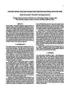
quite distinct trajectories (slow vs. fast, tight turn vs. wide turn, (9) etc.). Hence, fine-grain invariant signatures will recognize such patterns as different. However, these patterns are similar in that subject to the following constraints: they can all be described by the same sequence of semantic labels. To generate such a concise, semantic description, we (10) follow these steps (please consult [11] for further details): 1. Sensor data fusion. We employ the Kalman filter as a where is a constant larger than zero used as penalty for softsensor-data-integration tool. The Kalman filter helped in smooth- margin SVMs. According to the KKT conditions [2], the value ing the trajectories, fusing the trajectories from different camof has three ranges: eras, and providing velocity and acceleration estimates from : non-support vectors, the raw trajectories. : support vectors and , and 2. Event segmentation. We use an EM-based algorithm to : support vectors and . segment the fused trajectory from multiple cameras into segBy solving Equations 9 and 10, the class prediction funcments. These segments are homogeneous in terms of their tion is formulated as acceleration characteristics, which are assumed to be either (11) constant or linear in the magnitude or direction. 3. Trajectory summarization. Based on the acceleration statistics computed above, we assign each segment a semantic la3.2. Causes of Misclassification bel. For example, the stop condition is identified as zero Let us use SVMs to explain the boundary-skew problem. As acceleration and zero initial velocity. A half turn is identhe number of negative examples (the majority class) grows, so tified when (a vehicle makes a turn of approximately ). does the number of negative support vectors that exert influ3. BIASED STATISTICAL INFERENCE ence on an unlabeled instance. To illustrate this problem, we use a 2D checkerboard example. The checkerboard divides a As discussed in Section 1, event detection presents two chal200*200 square into four quadrants. The top-left and bottomlenges to a classifier: unequal class importance, and imbalright quadrants are occupied by negative instances and the topance in training classes. The imbalanced training-data problem right and bottom-left quadrants by positive instances. The lines arises when the negative instances are the norm and abundant, between the classes are the “ideal” boundary that separates the but the positive instances are rare. This imbalance situation two classes. causes the class boundary to skew toward the minority side, Figure 1 exhibits the boundary distortion between the two and hence results in a high incidence of false negatives. While left quadrants of the checkerboard under two different negathe skewed boundary is Bayes optimal when a prior distribution tive/positive training-data ratios. Figure 1(a) shows the SVM heavily favors the majority class, we must make adjustments to . Figure 1(b) shows the class boundary when the ratio is correct the skew when the risk of mispredicting a positive event boundary when the ratio is . The boundary in Figfar outweighs that of mispredicting a negative event. ure 1(b) is much more distorted compared to the boundary in In this section, we present alternatives to support biased staFigure 1(a), and hence causes more false negatives. tistical inference. We first provide a brief overview of SVMs to
+ £+ � Ø× £+ �
Ö
ÎÐÏ ÏÒÑ Ó¼ÔÕ Ä Â ² Î ® Ç mÅE�Æ Ç
+¯ × Ö Ö
� 1 Ù
Ú �¤E¦K²BÛ�±mܸ �Ä Ý m¥ ß9¥dàá�¤K®8¤9¥�¦R§â¨K¦�´ ¥ Å�Þ Ç
#
0
'ã W ##%W ã W W
set up sufficient context for discussions. (We use SVMs as our classifier because of their superior performance in many application domains.) We then explain the causes of misdetecting rare events. Finally, we present three alternatives that we will evaluate in Section 4. 3.1. SVM Overview We consider SVMs in a binary classification setting. We are , , ... , given a set of training data where is the training instance and its label, either for benign events or for hazardous events. SVMs separate these two classes by a hyperplane with maximum margin [2]. For nonlinearly separable cases, SVMs can project the training data onto a higher dimensional feature space via a Mercer kernel operator . In addition, Vapnik’s soft-margin theory [8] introduces slack variables to permit training error. Given , SVMs model class prediction as
5�
W
��k�� #� �� -� ��-#�
��-���K9� (
W
$ �� �¡�¢£�¤�¥�¦R§©¨K¦ ª/«¬I!¥b®¯!¥�ª�°9®�±9²³«k®µ´¶´·´·®�¸ ® (8) where ¹ is the norm to the hyperplane, º »¼º ½ºmº ¹|º¾º is the perpendicular distance from the hyperplane to the origin, and ¿ is an input-space to feature-space mapping function. The optimal solution of SVMs is formulated by maximizing the Lagrangian
3.3. Proposed Remedies We use two criteria for class-prediction evaluation: tradeoff between specificity and sensitivity, and overall classification accuracy. We define sensitivity of a learning algorithm as the ratio of the number of true positive (TP) predictions over the number of positive instances (TP+FN) in the test set, or Sensitivity = TP /( TP+FN). The specificity is defined as the ratio of the number of true negative (TN) predictions over the number of negative instances (TN+FP) in the test set, or Specificity = TN / (TN+FP). Our design goal is to improve sensitivity and at the same time maintain high specificity. In what follows, we present three methods for achieving our design goal. The first two methods, thresholding and penalty, aim to tackle the problem of unequal class importance, making a better tradeoff between specificity and sensitivity. The last method, conformal transformation, helps alleviate the drawback of imbalanced training data. 3.3.1. Thresholding Method A simple method for reducing false negatives is to change the decision threshold b in Equation 11. This shift trades specificity for sensitivity. The new decision function is
c=1000, sigma=26.0
c=1000, sigma=10.0
120
120
115
115
110
110
105
105
100
100
95
95
90
90
85
85
80 0
20
40
60
80
80 0
100
10
20
30
(a) 10:1
40
50
60
70
80
90
100
(b) 1000:1 Fig. 1. Boundary Distortion.
Ȍ
Ú �¤�¦-²BÛ�±mÜk¸ Ä Ý ¾¥ ß�¥dà��¤-®�¤9¥d¦R§¯¨Kä ¦�® ¥ Å9Þ Ç
(12)
where is the new threshold after boundary movement. We use thresholding as the yardstick to measure how the other methods perform.
Kernel-based methods, such as SVMs, introduce a mapping function which embeds the the input space into a highdimensional feature space as a curved Riemannian manifold � where the mapped data reside [3]. A Riemannian metric � � �� is then defined for , which is associated with the kernel function .
¿
ö
��-�
�� )�� " � ´ (16) Ë x ¦K² ÉÈ ç Ì x ® Ë x ¦ ¬ ç Ì x ® xË ¦ Å shows how a local area around x inxa is magThe metric nified in ö under the mapping of ¿ . The idea of conformal transformation in SVMs is to enlarge the margin by increas ��-� around ing the magnification factor the boundary (rep
�
�
3.3.2. Penalty Method Veropoulos [9] uses a soft margin technique with SVMs for controlling the trade-off between false positives and false negatives. The basic idea is to introduce different penalty functions for positively and negatively labeled instances, in which is assigned to the class in which misclasa larger multiplier sification carries a heavier cost. The Lagrangian formulation in Equation 9 is generalized with two penalty functions for falsepositive and false-negative errors as follows:
+
+
À ² æ·æ É æ·æ ç §B Ñéè Ä Â ¦9§B Ñîí �ê ë�ì�Å è Æ Â ¬ïÄ Â �ð � �¡¤9¥#§ñ¨K¦�¬C«£§©�¥¾òT¬ mÅEÆ Ç
Ä Â ¦ �ê ë�ì�Å í Æ Ä Ý ¥¾!¥�´ ¥ Å9Þ)ó
and vice versa.
3.3.3. Adaptibe Conformal Transformation (ACT) In [10], we proposed feature-space adaptive conformal transformation (ACT) for imbalance-data learning. We showed that by conducting conformal transformation adaptively to data distribution, and adjusting the degree of magnification based on feature-space distance (rather than based on input-space distance proposed by [1]), we can remedy the imbalance-data learning problem. A conformal transformation, also called a conformal mapping, is a transformation which takes the elements to elements while preserving the local angles between the elements after the mapping, where is the domain in which the elements reside [4].
úüû³ý
ý
�
���
�
�
resented by support vectors) and to decrease it around the other points. This could be implemented by a conformal transformation of the related kernel according to Eq. 16, so that the spatial relationship between the data would not be affected much [1]. Such a conformal transformation can be depicted as
��)�� " �
Ì x ® x ¦K² Ø x¦ Ø x ¦ Ì x ® x ¦�® (17) � � � � where ý is a properly defined positive conformal function. in a way such that the new Remaný � x� should be i� chosen � nian metric x , associated with the new kernel function � x � x" � , has larger values near the decision boundary. Furthermore, deal with the skew of the class-boundary, we magnify � x� tomore in the boundary area close to the minority class. �
Ñéè ª ª Î ô Ú ²õ§ È ® Ó#ÔÕ (14) Ñ í Ǫ -ª Î ô Ú ^E²³¬ È ´ (15) Ç Ö and Ö 7 are the penalty for the positive and negative 7 sides respectively. If Ö is larger than Ö , fewer positive data would be misclassified as negative data; thus öø÷ is reduced,
���
��
�
(13)
�
���
�
The dual formulation gives the same Lagrangian but with different constrained by
ù þÿû¯ù � ý � ú
���
��
��
��
�
�
�
��
�
Due to the space limitation, we cannot document the entire algorithm in this paper. Please refer to [10, 11] for details. 4. EXPERIMENTAL RESULTS We have conducted experiments on detecting suspicious events in a parking-lot setting to validate the effectiveness of our proposed methods. We report our results in two parts: the results on invariant descriptors, and the results on learning-method comparison. 4.1. Invariant Descriptors For experiments on fine-grain and coarse-grain invariancy, two cameras were used to record the activities in a parking lot. Fig. 2 shows some sample results of computing numeric invariant signatures. Fig. 2 (a) and (b) show the same motion sequence (a zig-zag or an M-pattern) captured from two different camera poses, and (c) shows the invariant signatures, computed using Eq. 7 (the dash-line curve for Fig. 2(a) and the
r
Æ To conserve space and to better illustrate the motion trajectories, we su-
perimposed multiple video frames into a single picture for display.
(a)
(b)
(a)
(b)
(c) (d) Fig. 2. (a) and (b) the same motion event captured by two different cameras, (c) invariant signatures computed based on using Eq. 7 (dash-line for (a) and solid-line for (b)), and (d) invariant signatures computed for a circling trajectory.
(c) (d) Fig. 3. Invariant descriptors for a zig-zag trajectory or an MPattern. (a) and (b) the snapshots of two cars performing a zig-zag motion in a parking lot; and (c) and (d) the computed invariant trajectory descriptors.
solid-line curve for Fig. 2(b)). We employed a simple mechanism for figure-background separation. Because in our current experiment the camera aims were fixed, we detected the presence of moving objects by performing a simple difference operation between adjacent video frames. We then extracted the moving objects by another difference operation with an adjacent video frame having no motion. As can be seen from the figure, the invariant signatures are very consistent even through the trajectories were captured from different viewpoints, and thus not directly comparable. Fig. 2(d) shows the invariant features for a circling trajectory. Again, the dash-line and solid-line curves represent the invariant signatures computed for the same motion trajectory recorded by the two cameras. From these results, we can see that numeric invariant features capture the essential traits of motion trajectories in a way that is not affected by the placement of cameras. The limitations of numeric invariant signatures are these: First, because the signatures capture the fine detail of a motion curve, it is best used for fine-grain correlation of the same motion trajectory imagined under varying conditions, such as different camera poses. Second, its numeric nature is difficult for a human operator to comprehend. Hence, for coarse-grain correlation of motion events, we resort to semantic invariant signatures that summarize motion events as a concatenation of semantically meaningful patterns, such as “right turn,” “left turn,” “constant speed,” “stop,” etc. Sample images for two zig-zag patterns, this time executed by two vehicles and recorded using two cameras placed at dif-
ferent locations, are shown in Fig. 3(a) and (b). The Kalman filter was used to track the moving vehicles. Sample raw and Kalman-filtered vehicle trajectories are shown in Fig. 3 (c) and (d) for Fig. 3 (a) and (b) respectively, where the black (dark) curve is the raw vehicle trajectory and the red (light) curve is the Kalman filtered and fused trajectory. In Fig. 4, we show the results of segmenting Kalman-filtered trajectories and computing their semantic invariant signatures. Fig. 4 depicts the magnitude � and direction � of the�� acceleration curves of the motion trajectories, and curves (whose sign was used to determine the turning direction) used in segmentation. The � and � trajectories estimated from the Kalman filter are shown in black, while the piecewise linear approximations of these curves using the EM algorithm described before are shown in red. Vertical lines show the beginning and end of each segment. For illustration, the boundaries between adjacent segments and the segment labels are shown in Fig. 3(c) and (d) as well. The results show that we can obtain similar semantic descriptions even when the M-patterns were executed by different vehicles and imaged by different cameras.
º º
�-t H� O N� �
º º
4.2. Learning Method Comparison In this experiment, we compared the sensitivity and specificity of three methods presented in Section 3.3. For surveillance applications, we care more about the sensitivity, and at the same time, would like to keep the specificity high. We recorded video at parking lot- � on UCSB campus. We collected trajectories depicting five motion patterns: circling (� instances), zigzag-pattern or M-pattern ( ��� instances), back-
#
i
(a) Sensitivity
(a) (b) Fig. 4. Segmentation of motion trajectories using the acceleration statistics shown here. (a), (b) corresponds to Fig. 3 (a) and (b), respectively.
�
i
¼#
and-forth (� instances), go-straight ( � instances), and parking ( � instances including additional synthetic data to sim�� ulate the skew effect). We divided these events into the benign and suspicious categories. The benign-event category consists of patterns go-straight and parking, and the suspicious-event category consists of the other three patterns. For each experiment, we chose �� of the data as the training set, and the remaining � �� as� our testing data. We employed the best kernel-parameter settings obtained through running a five-fold cross validation (see [11] for details), and report here the average class-prediction accuracy. Figure 5(a) presents the sensitivity of using SVMs, and of using the three improvement methods. All three methods, thresholding, penalty, and ACT improve sensitivity. Among the three, ACT achieves the largest magnitude of improvement over SVMs, around � percentile. Figure 5(b) shows that all methods maintain high specificity. Notice that the thresholding method performs well for detecting M-pattern and back-forth; however, it does not do well consistently over all patterns. The performance of the thresholding method can be highly dependent on the data distribution. The penalty method does not work effectively. The reason can be explained by the KTT condition presented in Section 3.1, where the parameter imposes only an upper bound on , not a lower bound. Changing does not necessarily affect after is increased to a certain degree; and consequently, the penalty method does not work well with SVMs.
W W
i
#
+
+
Ö
Ö
Ö
5. CONCLUSIONS AND FUTURE WORK We have described our invariant feature extraction component and improved statistical learning methods for dealing with the challenges of detecting rare events. Our experimental results showed that our proposed methods are effective. We plan to extend our methods to tackle the problem of multiple camera spatio-temporal data fusion. We will also conduct experiments in other event-detection settings.
(b) Specificity Fig. 5. Sensitivity and Specificity 6. REFERENCES [1] S. Amari and S. Wu. Improving support vector machine classifiers by modifying kernel functions. Neural Networks, 1999. [2] C. J. C. Burges. A tutorial on support vector machines for pattern recognition. Data Mining and Knowledge Discovery, 2(2), 1998. [3] C. J. C. Burges. Geometry and Invariance in Kernel Based Methods. In Adv. in Kernel Methods: Support Vector Learning. MIT Press, 1999. [4] H. Cohn. Conformal Mapping on Riemann Surfaces. Dover Pubns, 1980. [5] I. Pavlidis, V. Morellas, P. Tsiamyrtzis, and S. Harp. Urban surveillance systems: From the laboratory to the commercial world. Proc. of the IEEE, 89(10), 2001. [6] C. Regazzoni and P. K. Varshney. Multisensor surveillance systems based on image and video data. Proc. of the IEEE Conf. on Image Proc., 2002. [7] D. J. Struik. Differential Geometry. Addison-Wesley, Reading, MA, 2 edition, 1961. [8] V. Vapnik. The nature of statistical learning theory. Springer, New York, 1995. [9] K. Veropoulos, N. Cristianini, and C. Campbell. Controlling the sensitivity of support vector machines. Proceedings of the International Joint Conference on Artificial Intelligence, (IJCAI99), 1999. [10] G. Wu and E. Chang. Adaptive feature-space conformal transformation for learning imbalanced data. UCSB Technical Report http://www.mmdb.ece.ucsb.edu/ echang/act-fs.pdf, 2003. [11] G. Wu, Y. Wu, L. Jiao, Y.-F. Wang, and E. Chang. Multi-camera spatio-temporal fusion and biased sequence-data learning for security surveillance. UCSB Technical Report, April 2003. [12] Y. Wu, G. Wu, and E. Chang. A framework for detecting hazardous events. IS&T/SPIE International Conference on Storage and Retrieval for Media Databases, January 2003.