New edge-based feature extraction algorithm for video segmentation

New edge-based feature extraction algorithm for video segmentation Edmundo S´aeza , Jos´e M. Gonz´alezb , Jos´e M. Palomaresa , Jos´e I. Benavidesa and Nicol´as Guilb a Dept.

Electrical Engineering and Electronics, University of C´ordoba, C´ordoba, Spain b Dept. Computer Architecture, University of M´ alaga, M´alaga, Spain ABSTRACT

This work presents a new video feature extraction technique based on the Generalized Hough Transform (GHT). This technique provides a way to define a similarity measure between two different frames, which establishes the basis for scene cut detection algorithms. Moreover, GHT allows to calculate the differences between two frames in terms of rotation, scale and displacement. This provides a framework for the development of global motion estimation algorithms. In addition, gradual transition detection algorithms (fades, dissolves, etc.) can also be developed. To illustrate the posibilities of this technique, a scene cut detection algorithm is also proposed. This algorithm works with MPEG video in compressed domain, achieving real time processing. An improved thresholding technique is also stated. This technique uses two different sets of similarity values making the scene cut detection algorithm perform quite well with different types of videos. The thresholding process reports two different kinds of cuts: real cuts and probable cuts. Also, it detects the location of dynamic scenes, which can be used to perform further semantic analysis. Finally, the use of the improved thresholding technique and a set of optimized parameters results in an algorithm where no human intervention is needed. Several tests have been carried out using long videos, including more than 1400 cuts. Comparison with another well-known cut detection algorithm has also been performed. Keywords: feature extraction, Generalized Hough Transform, scene change detection, video segmentation, video indexing

1. INTRODUCTION ∗

Video databases have become more and more important due to the large amount of visual information they store. Decreasing prices in storage devices and the availability of higher communications bandwidth have made it possible to store very large video archives. In order to maintain such amount of information organized, tools are needed. There is a great number of tools that manipulate video information under human supervision for storage, playing and editing purposes. However, to be able to maintain video information efficiently, automatic organization tools are needed. The organization of video information is known as video indexing. The main objective of video indexing techniques is to get key frames from video streams in order to create video indexes. One of the most used techniques in video indexing is scene change detection. This technique allows to split the video into structural elements like shots, scenes, etc. To perform scene change detection, techniques for feature extraction from video sources should be developed. In fact, feature extraction is the basis to perform Corresponding authors: Edmundo S´ aez: E-mail: [email protected], Telephone: +34 957212062, Address: Escuela Polit´ecnica Superior, Avda. Men´endez Pidal s/n, 14071 C´ ordoba, Spain Nicol´ as Guil: E-mail: [email protected], Telephone: +34 952133327, Address: Departamento de Arquitectura de Computadores, Campus de Teatinos, P.O. Box 4114, 29080 M´ alaga, Spain ∗ Copyright 2003 Society of Photo-Optical Instrumentation Engineers. This paper was published in Image and Video Communications and Processing 2003 Proceedings and is made available as an electronic reprint with permission of SPIE. One print or electronic copy may be made for personal use only. Systematic or multiple reproduction, distribution to multiple locations via electronic or other means, duplication of any material in this paper for a fee or for commercial purposes, or modification of the content of the paper are prohibited.

many different tasks with video such as video indexing, video object segmentation, camera registration, object tracking, etc. Many works for feature extraction have been stated. One of their main application has been the development of scene cut detection algorithms. First works proposed different method for detecting scene change detection in uncompressed data. For example, Nagasaka et al.1 and Zhang et al.2 proposed three different algorithms: Pairwise pixel comparison, a pixel intensity based algorithm; Likelihood ratio, another pixel intensity based algorithm using statistical measures and picture block division; and finally Histogram comparison, a colour histograms based algorithm. Corridoni et al.3 proposed a very sophisticated evolution of the last one. This algorithm includes picture block division, statistical moments vectors, and an advanced thresholding technique known as adaptive thresholding.4 Abdel-Mottaleb5 proposed a method that is not based on chromatic but edge information. Finally, Zabih et al.6 proposed another edge based algorithm. It offers good results but at the cost of high computing time. Bimbo7 discusses several of these algorithms. Several methods for scene change detection in compressed domain have also been stated. Sethi and Patel 8 used only DC coefficients from I frames of MPEG compressed video in order to create luminance histograms. Liu et al.9 processed only information in P and B frames to detect scene changes. Meng et al. 10 used the variance of DC coefficients in I and P frames as well as motion vectors information. Zhang et al. 11 proposed a method using the pairwise difference of DCT coefficients. Yeo et al.4 used DC images† from the compressed video data to detect scene changes. They discussed successive pixel difference and color statistical comparison. Lee et al.12 proposed an edge based method that worked with compressed data by obtaining edge orientation and strength directly from the MPEG video stream. This work presents a new video feature extraction technique based on the Generalized Hough Transform (GHT). This technique provides a way to compare different frames from a video stream in order to obtain a similarity measure between them, establishing the basis for the development of a scene cut detection algorithm. It also allows to obtain the rotation, scale and displacement parameters between two frames, making it possible to develop global motion estimation algorithms or even gradual transition detection algorithms. To illustrate the possibilities of this technique, a scene cut detection algorithm is proposed. This algorithm presents four key characteristics that turn it into a very challenging one: 1. The ability to process video data in the MPEG compressed domain, using estimated values of DC coefficients,4 instead of real ones as other authors do. The use of estimated DC values makes the algorithm much faster because there is no need to perform the complete decompression process of a frame. 2. The use of two series of similariry values obtained from the video file, making the cut detection algorithm more robust against different types of videos. 3. The use of an improved thresholding technique, which includes specific analysis to find cuts where other techniques tend to miss them, especially in transitions from static to dynamic scenes or vice versa (see Sect. 3.2). Also, two different kinds of cuts are reported: real and probable cuts. 4. The improved thresholding technique and a set of optimized and well-tuned parameters result in an algorithm where no human intervention is needed, performing quite well with different kinds of videos. The paper is organized as follows. Section 2 gives an overview about the GHT and its application to feature extraction in digital video. Section 3 describes the application of the feature extraction technique to scene cut detection. Several experimental results and comparison with another technique are carried out in Sect. 4. Finally, conclusions are stated in Sect. 5. Some ideas about future work are given in Sect. 6. †

DC images are spatially reduced versions of the original images. The DC coefficients of the DCT transform are used to build these images.

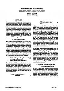
Figure 1. Variables defined in the GHT.

2. FEATURE EXTRACTION ALGORITHM 13

The Hough Transform was originally used to detect parametric shapes in binaries images. It is a very robust technique that can even be applied with missing or noisy data. Ballard14 generalized the Hough Transform to detect arbitrary shapes by computing a reference table used to calculate the rotation, scale and displacement of a template in an image. This technique had high memory and computational requirements. Thus, several improvements were proposed. One of the most interesting was proposed by Guil et al. 15 In that work, the detection process is split into three stages by uncoupling the rotation, scale and displacement calculation, achieving lower computational complexity. An evolution of this technique was presented in Ref. 16. A little review of the process will be done. However, a complete description is stated in Ref. 16. Let E be the edge points set in an image. The edge points of the image are characterized by the parameters (x, y, θ), where x and y are the point coordinates in two dimensional space and θ is the angle of the gradient vector associated to this edge point. An angle, ξ, called difference angle is also defined. Its value indicates the positive difference between the angles of the edge point gradient vectors that will be paired. All the variables abovementioned are shown in Fig. 1. From this description, three transformations will be defined. Let pi and pj be two edge points, (xi , yi , θi ) and (xj , yj , θj ) their associated information, and ξ the difference angle to pair points, transformation T can be written as follows: ½ (θi , αij ) θj − θi = ξ (1) T (pi , pj ) = 0 elsewhere where αij =

µ

¶ yi − y j 6 arctan θi , xi − x j

(2)

that is, αij is the positive angle formed by the line that connects pi and pj and the gradient vector angle of the point pi . Transformation S uses a similar expression to that in Eq. 1 to calculate the distance between the two paired points. This transformation is defined as follows: ½ (θi , αij , dij ) θj − θi = ξ S(pi , pj ) = (3) 0 elsewhere where dij =

q (xi − xj )2 + (yi − yj )2 .

Finally, transformation D uses an arbitrary reference point O and two vectors r~i and r~j : ½ (θi , αij , r~i , r~j ) θj − θi = ξ D(pi , pj ) = 0 elsewhere

(4)

(5)

360 α 0

θ

45º

360 α

θ

0

0 360

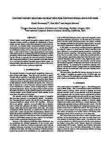
Figure 2. T OT of a rectangle.

where r~k = O − pk , k = i, j.

(6)

Transformation T can be used to compute the rotation angle β. The result of applying T transformation to the image is an image orientation table (IOT ) whose cells contain the pairings obtained. α and θ values are stored in rows and columns respectively. When a pairing with an αij and θj value is calculated, IOT [αij ][θj ] position is increased. Because different pairings might coincide with the same αij and θj values, the content of IOT [αij ][θj ] will indicate how many of them have these values. This transformation is also applied to the template to obtain a template orientation table (T OT ). α values are unaffected by rotation, scale and displacement, while θ is only affected by rotation. Then, if the template is included in the image, the T OT will be included in the IOT . If the template is rotated in the image, the T OT will be shifted circularly in the column direction in the IOT . Figure 2 shows the T OT of a rectangle, and the T OT of the same rectangle rotated 45 ◦ . When calculating IOT and T OT , several difference angles can be used, making it easier to work with special shapes, occlusions and/or noisy images. To obtain the value of β a special normalized cross correlation function is used. 17 A special correlation process is needed because sampling errors, noise or small deformations can make the paired points spread in a small window around the ideal (α, θ) value. Thus, correlation should be carried out using points in the T OT and small windows in the IOT . The expression of this special correlation is given below: P P T OT [α][θ − r] · W [IOT [α][θ]] (7) R(r) = α θ NI × NT where NI =

sX X α

NT =

sX X α

IOT [α][θ] · W [IOT [α][θ]]

(8)

T OT [α][θ] · W [T OT [α][θ]]

(9)

θ

θ

W [F [i][j]] =

XX

F [i + w1 ][j + w2 ].

(10)

w1 w2

Transformation S is invariant to displacement and proportional to scale. This transformation is applied to the template to obtain a template scale table (T ST ) which contains the distances between the paired points in the template. On the other side, transformation D is applied to the image to obtain an image displacement table (IDT ). The rotation angle β, computed in the previous step, is used to shift circularly the T ST . Then, cells in T ST and IDT with the same (α, θ) values are compared to obtain the scale factor. The distance between every pair of points in IDT [α][θ] is computed and compared with all the distances in T ST [α][θ] to vote in a one-dimensional accumulator array. Maxima in this accumulator indicate possible scale values.

(a) Frame 190

(b) Frame 191

(c) Frame 192

(d) Frame 193

Figure 3. Four consecutive frames from video sequence La Vita e Bella.

Finally, transformation D is applied to the template to obtain a template displacement table (T DT ). The rotation angle is used to shift it circularly. Non null cells in T DT and IDT with the same (α, θ) values are compared. Reference vectors stored in T DT [α][θ] are scaled and applied to the coordinates of the paired points in IDT [α][θ] to vote in a bidimentional space. The maximum position in this space will indicate the situation, in the image, of the reference point defined in the template shape. As it is explained above, this technique was originally designed to detect arbitrary shapes in binaries images. However, GHT can easily be applied to video processing. Let us assume that template and image are two different frames from a video stream. Thus, transformations T , S and D are applicable to this two frames, so rotation, scale and displacement values can be computed between them. To study the presence of a cut between two frames, the use of transformation T is enough. The correlation value used to obtain the rotation angle β is also a similarity measure between the two frames. Hence, a scene cut detector can be implemented just by studying this value along the different pairs of frames in the video. Moreover, the study of rotation, scale and displacement values along a window of n frames allows the development of global motion estimation algorithms.

3. SCENE CUT DETECTION ALGORITHM Using the feature extraction algorithm stated in Sect. 2, an advanced scene cut detection algorithm is presented here. As it is said in the previous section, the correlation value used to obtain the rotation angle, from the IOT and T OT tables obtained as a result of applying transformation T to the compared frames, is also a similarity measure between those two frames. Figure 3 shows four consecutive frames from a video sequence. There is a cut between frames 191 and 192. Figure 4 shows the IOT tables for frames in Fig. 3. As it can be seen, tables from Figs. 4(a) and 4(b) are quite similar, which results in a high correlation value. The same is applicable to tables from Figs. 4(c) and 4(d). However, tables from Figs. 4(b) and 4(c) are quite different, resulting in a low correlation value, which implies the existence of a cut. Our algorithm takes advantage of this fact. This method could be perfectly applied to uncompressed video sequences. However, full decompression of video and subsequent processing has two main drawbacks. On one hand, time is spent in performing the full

PSfrag replacements

PSfrag replacements 360

360

360 300

300 240

α

240 180

180 120

120 60

60

θ

(a) IOT for frame 190

360

360 300

300 240

α

180

180 120

120 60

60

360

PSfrag replacements

PSfrag replacements

300

300 240

α

180

180 120

120 60

60

θ

(b) IOT for frame 191

360

360 300

300

240

240

θ

α

(c) IOT for frame 192

240

240 180

180 120

120 60

60

θ

(d) IOT for frame 193

Figure 4. IOT for frames in Fig. 3.

decompression stage. On the other hand, the amount of data to be processed is considerably higher, increasing processing time. Here we propose to work with compressed video in order to obtain an algorithm able to perform scene cut detection in real time. The idea is to use DC images as a subsampled representation of the full frame. Once the DC image has been computed from the MPEG stream, the feature extraction technique is applied as usually. The process to obtain estimated values for all DC coefficientes for every frame in the video (type I, P or B) is stated in Ref. 4. In fact, tables from Fig. 4 have been calculated using DC images of frames in Fig. 3, instead of fully decompressed frames. The proposed algorithm consists of two different stages. In a first stage, the feature extraction technique is applied in order to calculate similarity values for every pair of frames in the video stream. Then, in the second stage, computed similarity values are analyzed through a thresholding process, reporting cuts location. Sections 3.1 and 3.2 describe in detail these two stages.

3.1. Calculation of similarity values Algorithm 1 describes the process to obtain the correlation values that indicate the similarity between each pair of frames in the video. It uses CannyEdgeDetector method to perform edge detection 18 on the DC image provided by ObtainDCImage. Parameters for the edge detection algorithm (paramsCED) include σ = 1 (gaussian standard deviation) and TH = 20 (threshold of edge pixels). Application of the feature extraction algorithm is implemented in method CalcIOTTable. Transformation T is applied to the DC image, resulting in an IOT table. Further correlation with the IOT table from the next frame is performed by CalcCorrelation. This method implements the special normalized cross correlation process shown in Eq. 7. It is important to take into account that method CalcIOTTable is called twice per iteration (lines 8 and 9), using two different sets of parameters: paramsIOT1 and paramsIOT2 . In both cases IOT table is discretized by 8 degrees in both directions. They also include two pairing angles instead of one. However, both pair of angles are different. The most suitable values are (90◦ ,180◦ ) and (90◦ ,135◦ ). Therefore, two correlation values are provided for each pair

Algorithm 1 Calculate correlation values 1: DCImage ← ObtainDCImage(M P EGF ile, f rame0 ) 2: edges ← CannyEdgeDetector(DCImage, paramsCED) 3: IOT11 ← CalcIOTTable(edges, paramsIOT1 ) 4: IOT12 ← CalcIOTTable(edges, paramsIOT2 ) 5: for i = 1 to numF rames do 6: DCImage ← ObtainDCImage(M P EGF ile, f ramei ) 7: edges ← CannyEdgeDetector(DCImage, paramsCED) 8: IOT21 ← CalcIOTTable(edges, paramsIOT1 ) 9: IOT22 ← CalcIOTTable(edges, paramsIOT2 ) 10: corrV alues1 [i − 1] ← CalcCorrelation(IOT11 , IOT21 ) 11: corrV alues2 [i − 1] ← CalcCorrelation(IOT12 , IOT22 ) 12: IOT11 ← IOT21 13: IOT12 ← IOT22 14: end for of frames. Hence, the algorithm returns two series of correlation values (corrV alues 1 and corrV alues2 ). This characteristic makes the algorithm perform quite well with different types of videos, because in some situations a cut can be missed by corrV alues1 but declared by corrV alues2 or vice versa. This way, the thresholding process is more likely to find cuts in difficult situations, at the cost of increasing the quantity of false alarms. Both series of correlation values (corrV alues1 and corrV alues2 ) will be the starting point for the second stage of the scene cut detection algorithm, the thresholding process.

3.2. Thresholding process Once the feature extraction technique has been carried out, a thresholding process has to be performed in order to determine where cuts are located. This work proposes a thresholding method that is an evolution of the one stated by Yeo et al. in Ref. 4. In that work, a sliding window is used. A cut is detected if the central element in the window is n times lower than the lowest value in the window, excluding the element in the midst of the window. This method is usually very effective, especially when transitions between static scenes are being analysed. A static scene19 is one that exhibits rather low motion from the objects in the scene and reduced camera motion as well. However, when a transition between static and dynamic scenes 19 (fast objects or camera movement) occurs, Yeo’s thresholding algorithm tends to fail. The reason is that, in dynamic scenes, correlation values are rather unstable. In such conditions, Yeo’s method would fail in the detection of cuts because it is highly probable that, when correlation values for border frames between static and dynamic scenes are being analysed, the sliding window contains very low values from the dynamic scene. In this work, a thresholding method that successfully deals which such transitions is proposed. In addition, the proposed thresholding method reports two different kinds of cuts: real cuts, where cut conditions are clearly satisfied, and probable cuts, where a cut is supposed to be, but it could be a false alarm. Proposed method consists of two stages. The first (Sect. 3.2.1 and 3.2.2) performs the individual analysis of corrV alues1 and corrV alues2 , detecting cuts and dynamic scenes in each serie of correlation values. The second (Sect. 3.2.3) combines both analyses, resulting in a final list of detected effects. 3.2.1. Detecting real and probable cuts Let c be the central element in a 21 frame sliding window. Let m be the element in the window with the lowest value (excluding c). A real cut (CUT) is declared if c/m < TR , where TR = 0.85. However, the use of a second parameter (TP = 0.93) allows the detection of probable cuts (CUTP). If TR ≤ c/m < TP a probable cut is declared. Figure 5(a) shows that two real cuts have been declared in frames 5362 and 5688 as a result of analysing corrV alues1 . On the other hand, Fig. 5(b) shows that analysis of corrV alues2 reports three real cuts (frames 5362, 5527 and 5688) and one probable cut (frame 5613).

1

1

0.9

0.9

0.8

0.8

0.7

0.7 CUT SDT

CUT

0.6 Correlation

0.6 Correlation

CUTP

DST

0.5 CUT

CUT

0.4

0.3

0.3

0.2

0.2

0.1

0.1

(a) Computed correlation values using paramsIOT1

DST CUT

0.4

0 5300 5325 5350 5375 5400 5425 5450 5475 5500 5525 5550 5575 5600 5625 5650 5675 5700 5725 Frame

SDT

0.5

0 5300 5325 5350 5375 5400 5425 5450 5475 5500 5525 5550 5575 5600 5625 5650 5675 5700 5725 Frame

(b) Computed correlation values using paramsIOT2

Figure 5. Subset of corrV alues1 (a) and corrV alues2 (b) from video sequence CNN.

ef fA CUT CUT CUT CUTP CUTP

+ + + + + +

ef fB CUT CUTP NONE CUTP NONE

= = = = = =

ef f CUT CUT CUTP CUTP NONE

Table 1. Resulting effect after combining effects from corrV alues1 and corrV alues2 (the order is not relevant). CUT means real cut, CUTP is probable cut, and NONE stands for no effect detected.

3.2.2. Detecting dynamic scenes Up to this point, the thresholding process is quite similar to the method stated by Yeo et al. However, first stage also marks transitions from static to dynamic scenes (SDT) as well as transitions from dynamic to static scenes (DST). Let mL be the lowest value to the left of c in the window. Let mR be the lowest value to the right of c in the window. A SDT is declared when c < TM , mL ≥ TM and mR < TM . Similarly, a DST is declared when c < TM , mL < TM and mR ≥ TM . TM is usually given a value of 0.65. Figures 5(a) and 5(b) show a dynamic scene that has been detected between frames 5466 and 5491 in both corrV alues 1 and corrV alues2 . 3.2.3. Combining individual analyses Once the individual analysis has been performed, it is necessary to combine both series of detected effects in order to obtain a final list of effects for the video that is being analysed. Rules for combining effects are shown in Tbl. 1. The order in which the effects are combined is not relevant, i.e. CUT + NONE = NONE + CUT = CUTP. Fig. 5 will be used to illustrate this stage. Frame 5362 has been marked as CUT in both corrV alues 1 and corrV alues2 . Then, the algorithm will declare a real cut in that frame. The same occurs in frame 5688. Frame 5527 has been marked as CUT in corrV alues2 but no effect has been detected processing corrV alues1 . Thus, a probable cut will be reported in that frame as final effect. Finally, neither real nor probable cut will be declared in frame 5613. It is also possible that CUT or CUTP in one serie of correlation values occur in the same frame that SDT or DST in the other. In that case, CUT or CUTP (depending on the type of cut detected) is set for that frame. Eventually, the frames between the SDT and DST marks belong to a dynamic scene, which is supposed to be delimited by cuts. Let a dynamic scene in corrV alues1 start at frame i1 and end at frame i2 . Let a dynamic scene in corrV alues2 start at frame j1 and end at frame j2 . Probable cuts are declared in frames

Sequence La Vita e Bella Dias Contados Don’t Say a Word Friends CNN Norman Normal

Sequence type Comedy movie Action movie Action movie Situation comedy News Cartoons

Duration 9:40 3:36 21:24 17:05 13:55 20:03

Number of frames 14523 5419 32100 25641 20876 30095

Number of cuts 132 32 517 299 116 360

Table 2. Video sequences used in the experiments.

DSST ART = max(i1 , j1 ) and DSEN D = min(i2 , j2 ) if and only if DSEN D − DSST ART ≥ DSM inLength , where DSM inLength = 10 frames. In Fig. 5, both series of correlation values mark frames 5466 and 5491 with SDT and DST respectively. Then, DSST ART = max(5466, 5466) = 5466 and DSEN D = min(5491, 5491) = 5491. Hence, as 5491 − 5466 ≥ DSM inLength , frames 5466 and 5491 are marked as probable cuts. The use of parameter DSM inLength is imposed to avoid short motion in the current scene to be considered as a dynamic scene, which is supposed to last for at least 10 frames. The reason for declaring probable cuts instead of real ones is that it is possible that punctual high motion in a static scene could be considered as a dynamic scene. It can be seen that the proposed scene cut detection algorithm make use of several parameters. That is also very common in other works. However, while other algorithms need a fine tuning of their parameters in order to perform satisfactorily, proposed parameter values make our algorithm perform quite well with different types of videos. Thus, it can be considered that no run time parameters need to be tuned, obtaining in this way an algorithm suitable for performing scene cut detection on different kinds of videos where no human intervention is needed.

4. EXPERIMENTAL RESULTS This section evaluates the performance of the proposed feature extraction technique applied to scene cut detection (HC). In addition to the proposed algorithm, a version that works with uncompressed video has also been implemented (HU). In order to test the efficiency of the proposed algorithm against existing cut detection methods, scene cut detector proposed by Corridoni et al. in Ref. 3 has been implemented as well (CHMC). This algorithm has been selected for comparison purposes because it offers good reliability and a high processing speed. All the implemented algorithms have been tested using the video sequences summarized in Tbl. 2. This sequences include more than 1400 cuts in almost 90 min. of video. The hardware configuration used to run the tests consists of an AMD Athlon K7, 1 GHz, 256 MB RAM, running Linux 2.2.16. The algorithms have been codified using the GNU g++ compiler version 2.95.2.

4.1. Performance parameters Several performance measures has been defined to evaluate scene cut detection algorithms. One of the most used is recall and precision values. Recall defines the percentage of correct detections in relation to the overall scene cuts in the video. Precision defines the percentage of correct detections in relation to the overall scene cuts detected by the algorithm. Mathematical expressions for this parameters are given below: Recall (%)

=

Precision (%)

=

c c+m c 100 · c+f 100 ·

(11) (12)

where c is the number of correct detections, m is the number of missed detections, and f is the number of false detections.

Sequence La Vita e Bella Dias Contados Don’t Say a Word Friends CNN Norman Normal

C(Pr) 132(3) 31(2) 480(42) 297(23) 113(7) 344(28)

HC M 0 1 37 2 3 16

F(Pr) 0 10(8) 78(62) 1(1) 14(2) 48(38)

C(Pr) 132(3) 32(2) 488(43) – – –

HU M 0 0 29 – – –

F(Pr) 2(0) 7(6) 63(55) – – –

CHMC C M F 132 0 296 30 2 38 462 55 84 285 14 0 100 16 26 344 16 330

Table 3. Details about correct (C), missed (M) and false (F) cut detections for each implemented scene cut detection algorithm. Figures in parenthesis indicate the overall effects marked as probable.

4.2. Statistics Results obtained from the execution of the implemented algorithms using the video sequences in Tbl. 2 are shown in Tbl. 3. HC algorithm reports very good results for all sequences. The amount of missed and false detections in sequences Don’t Say a Word and Norman Normal is higher than the others due to the length of the sequences and also the high motion existing in the videos. The same is applicable to sequence Dias Contados, which presents an elevated number of false detections. CNN reports 14 false detections (2 of them marked as probable cuts). However, 12 of them were caused by the abrupt irruption of big text captions in the image, which is very common in news videos. Note that, in sequences where motion is not dominant (La Vita e Bella, Friends, and maybe CNN), cuts marked as probable tend to be real cuts. On the other hand, in high motion videos an exhaustive analysis of probable cuts has to be done. This algorithm allows scene cut detection in real time, being able to process more than 25 fps. Algorithm HU has only been tested using three video sequences. The reason is that sequences Friends, CNN, and Norman Normal have been recorded directly from TV. TV channels normally mark their video broadcasts with a TV channel logo. Taking into account that the logo is continuously present in all the frames of a video, this element tends to alter the similarity values used to compare two frames. Thus, for this kind of videos, a previous processing is needed in order to remove TV channel logo. Sequences analysed with HU algorithm yield even better results, cutting down considerably the amount of missed and false detections. However, HU does not allow real time processing, as it takes about 1 second to process each pair of frames. In spite of its computing time limitations, it is an interesting alternative when efficiency plays a more important role than computing time. Tests performed with CHMC algorithm have been carried out using parameter values stated by the authors. Reported results are acceptable for some sequences but questionable for many others. In some sequences (La Vita e Bella and Norman Normal) the amount of false detections is excessive. In fact, obtained results report equal or higher amount of missed and false detections than HC. Fine tuning of parameter values would produce better results. However, HC and HU report quite good results, while no parameters need to be tuned. Real time processing using CHMC is not possible in any case. About 0.15 seconds are spent in processing each pair of frames. Recall and precision values obtained are shown in Tbl. 4. Two different cases has been considered for algorithms HC and HU. In case 1, no difference is made between real and probable cuts: all probable cuts are considered as real cuts. On the other hand, case 2 ignores all probable cuts. When case 2 is considered, precision is increased while recall is reduced. Although, sometimes, too many cuts are missed. Thus, it is preferable to consider probable cuts and maybe perform an exhaustive analysis of them.

5. CONCLUSIONS This work presents a new video feature extraction technique based on the GHT. This technique establishes the basis for the development of video segmentation algorithms, from scene cut detectors to global motion estimation algorithms. Gradual transition detectors can also be developed. To illustrate the possibilities of this technique, a sophisticated scene cut detection algorithm is proposed. This algorithm is able to perform scene cut detection

Sequence La Vita e Bella Dias Contados Don’t Say a Word Friends CNN Norman Normal

HC Case 1 Case 2 R P R P 100 100 97.73 100 96.88 75.61 90.63 93.55 92.84 86.02 84.72 96.48 99.33 99.66 91.64 100 97.41 88.98 91.32 89.83 95.56 87.76 87.78 96.93

HU Case 1 Case 2 R P R P 100 98.51 97.73 98.47 100 82.05 93.75 96.77 94.39 88.57 86.07 98.23 – – – – – – – – – – – –

CHMC R 100 93.75 89.36 95.32 86.21 95.56

P 30.84 44.12 84.62 100 79.37 51.04

Table 4. Statistics for algorithms HC, HU and CHMC in terms of Recall (R) and Precision (P) (in %). Case 1: Considering all probable cuts as real cuts. Case 2: Ignoring all probable cuts.

directly on MPEG compressed video, providing two different sets of similarity values, both of which are analysed using an advanced thresholding technique which is also presented here. As a result, the list of cuts reported by the algorithm consists of two different kinds of cuts: probable cuts and real cuts. Also, parameter values supplied make this algorithm perform quite well with different kinds of videos. This avoids the problem of choosing the correct parameter values depending on the video that is about to be analysed. Up to six video sequences have been used in order to test the efficiency of the proposed algorithm. These video sequences include more than 1400 cuts in almost 90 min. of video. For comparison purposes, a version of the proposed algorithm that works with uncompressed video has also been implemented, as well as another well-known scene cut detector proposed by Corridoni and Del Bimbo in 1998 (CHMC). Absolute figures as well as recall-precision statistics has been obtained for each implemented algorithm and video sequence. Statistics show that our algorithm (in both versions) clearly outperforms CHMC, yielding very interesting results. It also satisfies real time processing requirements.

6. FUTURE WORK Once that the feature extraction technique has been stated and a scene cut detector has been developed, future work will concentrate in the application of this technique to the development of global motion estimation algorithms. In fact, much work has been done and promising results are already being obtained. After that, gradual transition detection algorithms will also be studied.

REFERENCES 1. A. Nagasaka and Y. Tanaka, “Automatic video indexing and full-video search for object appearances,” in IFIP Proc, Visual Database Systems, 2, pp. 113–127, Elsevier Science Publishers B.V. (North-Holland), 1992. 2. H. J. Zhang, A. Kankanhalli, and S. W. Smoliar, “Automatic partitioning of full-motion video,” Multimedia Systems 1(1), pp. 10–28, 1993. 3. J. Corridoni and A. del Bimbo, “Structured representation and automatic indexing of movie information content,” Pattern Recognition 31(12), pp. 2027–2045, 1998. 4. B. Yeo and B. Liu, “Rapid scene analysis on compressed videos,” IEEE Trans. on Circuits and Systems for Video Technology 5(6), pp. 533–544, 1995. 5. M. Abdel-Mottaleb, “Image retrieval based on edge representation,” in ICIP 2000, 3, pp. 734–737, (Vancouver, Canada), September 2000. 6. R. Zabih, J. Miller, and K. Mai, “Feature-based algorithm for detecting and classifying scene breaks,” in ACM Multimedia 95, pp. 189–200, (San Francisco, California), November 1995. 7. A. Bimbo, Visual information retrieval, Morgan Kaufmann, California, 1999.

8. I. K. Sethi and N. V. Patel, “A statistical approach to scene change detection,” in IS&T/SPIE Symposium Proceedings, Storage and Retrieval for Image and Video Databases III, 2420, pp. 329–339, (San Jose, California), February 1995. 9. H. Liu and G. Zick, “Scene decomposition of mpeg compressed video,” in IS&T/SPIE Symposium Proceedings, Digital Video Compression: Algorithms and Technologies, 2419, pp. 26–37, (San Jose, California), February 1995. 10. J. Meng, Y. Juan, and S. Chang, “Scene change detection in an mpeg compressed video sequence,” in IS&T/SPIE Symposium Proceedings, Digital Video Compression: Algorithms and Technologies, 2419, pp. 14–25, (San Jose, California), February 1995. 11. H. Zhang, C. Low, and S. Smoliar, “Video parsing and browsing using compressed data,” Multimedia Tools and Applications 1(1), pp. 89–111, 1995. 12. S.-W. Lee, Y.-M. Kim, and S. W. Choi, “Fast scene change detection using direct feature extraction from MPEG compressed videos,” IEEE Transactions on Multimedia 2(4), pp. 240–254, 2000. 13. P. Hough, “A method and means for recognizing complex patterns,” 1962. U.S. Patent No. 3,069,654. 14. D. Ballard, “Generalizing the hough transform to detect arbitrary shapes,” Pattern Recognition 13(2), pp. 111–122, 1981. 15. N. Guil and E. Zapata, “A fast generalized hough transform,” in European Robotic and Systems Conference, pp. 498–510, (M´alaga, Spain), 1994. 16. N. Guil, J. Gonz´alez, and E. Zapata, “Bidimensional shape detection using an invariant approach,” Pattern Recognition 32, pp. 1025–1038, 1999. 17. J. Gonz´alez, N. Guil, and E. Zapata, “Detection of bidimensional shapes under global deformations,” in X European Signal Processing Conference (EUSIPCO 2000), (Tampere, Finland), September 2000. 18. J. Canny, “A computational approach to edge detection,” IEEE Transactions on Pattern Analysis and Machine Intelligence 8, pp. 679–698, November 1986. 19. C.-L. Huang and B.-Y. Liao, “A robust scene-change detection method for video segmentation,” IEEE Trans. on Circuits and Systems for Video Technology 11(12), pp. 1281–1288, 2001.