The general theory, based on spherical harmonics and. Bessel functions, is illustrated with a spherically symmetric source example. 2. The inverse source ...
J. Opt. A: Pure Appl. Opt. 2 (2000) 179–187. Printed in the UK
PII: S1464-4258(00)09132-7
Inverse source problem with regularity constraints: normal solution and nonradiating source components Edwin A Marengo and Richard W Ziolkowski Department of Electrical and Computer Engineering, The University of Arizona, Tucson, AZ 85721, USA Received 1 November 1999 Abstract. The use of regularity constraints in formulating the scalar inverse source problem
(ISP) is investigated. Two kinds of regularity constraints are considered: compact supportness in a given source region, and normal differentiability on the boundary of that region. Normal solutions (minimum L2 norm solutions) to the ISP for square-integrable (L2 ) scalar sources with and without the above-mentioned regularity constraints are derived and compared. The (generally nontrivial) nonradiating parts of the corresponding normal solutions are evaluated. Keywords: Inverse source problem, nonradiating sources
Helmholtz equation
1. Introduction
A problem of considerable interest for the object reconstruction branches of the wave disciplines (such as optics and acoustics) is the so-called inverse source problem (ISP) [1–3]. In its usual form, the ISP consists of deducing a source of known support, say D, from knowledge of its generated field outside D. Different aspects of this problem have been investigated by M¨uller [4], Moses [5, 6], Friedlander [7], Bleistein and Cohen [1], Hoenders [8], Devaney [9], Devaney and Porter [2, 3], LaHaie [10, 11], Carter and Wolf [12], Wolf [13], Bertero [14], Marengo and Devaney [15] and Marengo et al [16, 17]. Attention has been given to both the scalar and electromagnetic cases, for both deterministic and random sources. The focus has been on the fundamental nonuniqueness question [18] and a priori constraints that may render the ISP unique. The latter include the constraint of minimizing the solution’s L2 norm, which has lead to the so-called minimum energy solutions [2, 3]. Applications include inverse scatteringbased surveys [18–21], holographic imaging [2, 3, 22] and antenna design [4]. The time-dependent ISP with far-field data has also received attention recently as an analogue of the limited-view Radon inversion problem that arises in the formalism of computerized tomography [16]. This work is concerned with the ISP for deterministic square-integrable (L2 ) scalar sources ρ contained within a spherical volume V = {r ∈ R 3 |r 6 a} of radius a, with centre at the coordinate origin. The focus is on the use of a priori regularity (smoothness) constraints in formulating the ISP. The formulation is based on the inhomogeneous 1464-4258/00/030179+09$30.00
© 2000 IOP Publishing Ltd
(∇ 2 + k 2 )ψ(r ) = −4πρ(r )
(1)
in three-dimensional space. The field ψ(r ) generated by a source ρ(r ) is then given by the familiar outgoing Green function integral Z 0 eik|r−r | . (2) ψ(r ) = d3 r 0 ρ(r 0 ) |r − r 0 | We review first the ISP for general L2 (V ) sources, and examine later the ISP for L2 (V ) sources with additional regularity constraints. We are particularly interested in L2 (V ) sources ρ that possess compact support in the source volume V , for which ρ(r ) = 0 on the boundary ∂V = {r ∈ R 3 |r = a} of V . We shall also consider the more regular class of L2 (V ) sources of compact support V whose normal derivatives also vanish on the boundary ∂V of V . The results presented in this paper provide, to our knowledge, the first investigation of ISPs with such regularity constraints. Extension to yet more regular classes of sources, although not to be considered here, follows lines similar to those provided here for the cases above. A unique solution to the usual ISP for general L2 (V ) sources, without additional constraints, cannot be obtained due to the presence of nontrivial nonradiating (NR) sources [1, 7, 23] localized within the source volume V . In particular, the field produced by a localized NR source vanishes outside the source’s support. It then follows that, without additional pieces of information about the field and/or the source, the NR source components of a source 179
E A Marengo and R W Ziolkowski
cannot be deduced from knowledge of its exterior field. The usual ISP admits a unique solution if one imposes the additional constraint of minimizing the source’s L2 norm. The solution in question is the usual minimum energy solution [2, 3], also known as ‘the normal solution’ in linear inversion language [14]. Physical interpretations of these normal solutions have been given in [2, 3, 22] in the context of generalized holography. Normal solutions to the usual ISP are orthogonal to all L2 NR sources confined within the source region, i.e., they lack a NR part [2, 3]. It is shown in this paper that, in contrast, by imposing additional regularity constraints to the usual ISP, one can actually extract NR source components of the unknown source. In particular, we derive expressions for the normal solutions corresponding to ISPs with regularity constraints, along with their (generally nontrivial) NR source contributions. We thus examine a means of extracting NR source components of an unknown radiating (or scattering) object that is known a priori to be reasonably well behaved in a sense specified by given regularity constraints. We then also illustrate the use of a priori information in formulating the ISP. The latter question had been investigated, for other forms of a priori information, by Moses [5, 6] and Bleistein and Cohen [1]. In addition, the present analysis also corroborates, for the special case of L2 sources contained in the spherical volume V , a recent result derived in [17] which states that any L2 source of compact support having vanishing normal derivatives on the boundary of its support must possess a NR part. The general theory, based on spherical harmonics and Bessel functions, is illustrated with a spherically symmetric source example. 2. The inverse source problem for L2 (V ) sources
In this section, we formulate, by means of a general linear inversion formulation, the ISP for L2 sources ρ of support V = {r ∈ R 3 |r 6 a} (such that ρ(r ) = 0 if r > a). The general approach developed in this section will be specialized in section 3 to L2 (V ) sources with various degrees of regularity on the boundary ∂V = {r ∈ R 3 |r = a} of the source volume V . In the present section, we also consider the unique decomposition of a source into its radiating and NR parts in the Hilbert space X of L2 (V ) sources with the defined inner product Z (ρ, ρ 0 )X = d3 rρ ∗ (r )ρ 0 (r ) (3) V
where ∗ denotes the complex conjugate. The general source decomposition results developed here will find use in section 4 in connection with a spherically symmetric source example. We will then illustrate how the NR source components become, in general, increasingly noticeable as one imposes stricter source regularity properties. In particular, it will be shown that normal solutions to ISPs with regularity constraints contain, in general, NR source components in the Hilbert space X. It is well known [24] that for r > a the field ψ(r ) radiated by a source ρ ∈ X can be expressed in the multipole 180
expansion form ψ(r ) = ik
l ∞ X X
gl,m h(1) l (kr)Yl,m (rˆ )
(4)
l=0 m=−l
where rˆ ≡ r /r, h(1) l (·) is the spherical Hankel function of the first kind and order l (as defined in [24], p 740), and Yl,m (·) is the spherical harmonic of degree l and order m (as defined in [24], p 99). The expansion coefficients gl,m in equation (4) are the multipole moments and are defined by the inner products gl,m = (ψl,m , ρ)X
(5)
where ψl,m (r ) = 4π H (a − r)jl (kr)Yl,m (rˆ ) l = 0, 1, . . . ;
m = −l, −l + 1, . . . , l
(6)
where jl (·) is the spherical Bessel function of the first kind and order l (as defined in [24], p 740) and H (·) is Heaviside’s unit step function. The field for r > a defined by equation (4) is uniquely determined by the multipole moments. Because of this, in the following we formulate the ISP of deducing the L2 (V ) source with minimum L2 norm that is consistent with a given data . We assume the latter to vector g = {gl,m } having entries P gl,mP l 2 be square-summable so that ∞ l=0 m=−l |gl,m | < ∞. We also define the discrete Hilbert space Y of all such squaresummable data vectors and assign to it the inner product (g , g 0 )Y =
l ∞ X X
∗ 0 gl,m gl,m .
(7)
l=0 m=−l
To address the ISP in this framework, we define, by using equation (5), the linear source-to-data vector mapping Pρ = g
(8)
which assigns to each source ρ ∈ X a data vector g ∈ Y according to the rule (Pρ)l,m = (ψl,m , ρ)X .
(9)
The class of L2 NR sources of support V is exactly the null space N(P ) of the linear mapping P [1, 23]. In the following, we shall assume the field for r > a and, in particular, its corresponding data vector g , to be realizable from L2 (V ) sources. In mathematical language, we require the data vector g to be in the range of the linear source-to-data vector mapping associated with the source space L2 (V ). The range in question has been defined explicitly in [17] by using the so-called Picard conditions [14] that apply to this ISP. In particular, the range R(P ) of P consists of the data vectors g that obey the necessary and sufficient condition l ∞ X X
|gl,m |2 /σl2 < ∞
(10)
l=0 m=−l
where
Z
a
σl2 ≡ (4π )2
drr 2 jl2 (kr) 0
= 8π 2 a 3 [jl2 (ka) − jl−1 (ka)jl+1 (ka)].
(11)
Inverse source problem with regularity constraints
Under this condition, the normal solution to the ISP, corresponding to the unique source ρˆ of minimum L2 norm (minimum energy) associated with a given data vector g , is defined by the pseudoinverse of P and is given by [14] ρˆ = P † (P P † )−1 g (Pρ, g )Y = (ρ, P g )X .
(P † g )(r ) =
gl,m ψl,m (r ).
(14)
l=0 m=−l
It is not hard to show by using equations (6), (9), (11), (12), (14) and the orthogonality property of the spherical harmonics that l ∞ X X ρ( ˆ r) = gl,m ψl,m (r )/σl2 l=0 m=−l
= 4π H (a − r)
l ∞ X X
gl,m jl (kr)Yl,m (rˆ )/σl2 .
(15)
l=0 m=−l
The normal solution ρˆ given by equation (15) consists of a source-free multipole expansion, over the truncated spherical wavefunctions ψl,m , with multipole moments gl,m /σl2 . Expression (15) can be shown to be in the form of the usual singular system representation of the normal solution associated with the linear mapping P [1, 14]. The terms σl2 are known to decay exponentially fast for l > ka, confirming the ill-posed nature of the ISP [14]. The ISP results presented above can be used to uniquely decompose a source ρ in the Hilbert space X into its radiating and NR source components. In particular, it is a wellestablished fact [2, 3, 14] that any source ρ ∈ X can be uniquely decomposed into the sum ρ = ρˆ + ρNR of a radiating and a NR part, ρˆ and ρNR respectively, where ρ( ˆ r) is exactly the normal solution in equation (15) corresponding to the data vector produced by the given ρ. The normal solution to the ISP formulated above, in which we imposed no regularity constraints, thus lacks a NR part in the Hilbert space X. In section 3, we will depict a different scenario for ISPs with regularity constraints. We will show then that normal solutions to such ISPs do contain, in general, NR source components in the Hilbert space X. We will also illustrate an interesting result derived in [17] which states that any L2 source of compact support having vanishing normal derivatives on the boundary of its support must possess a NR part. 3. The inverse source problem for L2 (V ) sources with regularity constraints
In this section, we consider L2 sources ρ that are compactly supported in the spherical volume V = {r ∈ R 3 |r 6 a} (such that ρ(r ) = 0 if r > a). Any such source must admit a representation of the form ρ(r ) =
L ∞ X X L=0 M=−L
qL,M (r)YL,M (rˆ )
(16)
∞ X
a(n, L, M; v)ρn;v (r)
(17)
n=0
where
(13)
The latter is found from equations (3), (7), (9), (13) to be given by l ∞ X X
qL,M (r) =
(12)
where P † is the adjoint of the linear mapping P , defined by †
where qL,M (r) is an r-dependent function that can be expanded in the Fourier–Bessel series form
ρn;v (r) =
p 2/a 3 H (a − r)jv (βv,n r/a) |jv+1 (βv,n )|
(18)
where v is an arbitrary non-negative integer. The parameters βv,n in equation (18) are consecutive zeros of the spherical Bessel function jv (·), i.e. jv (βv,n ) = 0, n = 0, 1, 2, . . . . The functions ρn;v (r) are orthonormal over V . The expansion coefficients a(n, L, M; v) associated with a given qL,M (r) are then (19) a(n, L, M; v) = (ρn;v , qL,M )X . In deriving these results we have made use of the completeness and orthogonality of the spherical harmonics YL,M (·) over the unit sphere, the completeness of the spherical Bessel functions jv (βv,n r/a) for fixed non-negative integer v and variable index n over the interval [0, a] for functions that vanish at r = a (see equation (11.51) of [25]), and the orthogonality property of the set of ordinary Bessel functions Jv (βv,n r/a) for fixed non-negative integer v and variable index n in the r-interval [0, a] (see equation (11.168) of [25]). Now, the non-negative integer v in equations (16)– (19) is arbitrary. For our purposes, the particular choice v = L > 0 will prove to be especially useful. With this choice, expressions (17)–(19) become qL,M (r) =
∞ X
a(n, L, M; L)ρn;L (r)
(20)
n=0
where p 2/a 3 H (a − r)jL (βL,n r/a) ρn;L (r) = |jL+1 (βL,n )|
(21)
and a(n, L, M; L) = (ρn;L , qL,M )X .
(22)
The above results will enable us to formulate the ISP for L2 sources that possess compact support in the source volume V by means of a linear inversion formalism analogous to that employed in section 2 for general L2 (V ) sources. In the following, we shall denote as L(0) 2 (V ) ⊂ L2 (V ) the class of L2 sources that are compactly supported in V . From the general results of section 2 and equations (16), (20)–(22), the ISP for L(0) 2 (V ) sources can be shown to reduce to finding the source expansion coefficients a(n, L, M; L) from knowledge of the multipole moments gl,m of the source’s exterior field. The relevant linear source expansion vector-to-data vector mapping is determined by substituting from equations (16), (20)–(22) into (5), (6). With these observations, we proceed next to evaluate the normal solution to the ISP investigated here (with the additional compact supportness constraint). By analogy with the procedure employed in section 2 for general L2 (V ) sources, we introduce the discrete Hilbert 181
E A Marengo and R W Ziolkowski
space U of source expansion vectors a = {a(n, L, M; L)} that are square-summable so that ∞ X L ∞ X X
a(n, ˆ L, M; L) = P † (PP † )−1 g .
Z |a(n, L, M; L)| =
d r|ρ(r )| < ∞,
2
3
2
V
n=0 L=0 M=−L
(23) and assign to it the inner product ( a , a 0 )U =
the source expansion vector aˆ corresponding to the normal solution ρˆ (0) is defined by the pseudoinverse of P :
∞ X L ∞ X X
a ∗ (n, L, M; L)a 0 (n, L, M; L).
The linear operator PP † : Y → Y is found from equations (30), (31) to be defined by ∞ X 2 αl,n . (33) (PP † g )l,m = gl,m n=0
It then follows that
n=0 L=0 M=−L
(24) We also recall here the definition, given in connection with equation (7), of the discrete Hilbert space Y of squaresummable data vectors g having multipole moment entries gl,m . With these Hilbert space definitions, we introduce next, also by analogy with the procedure employed in section 2, the linear source expansion vector-to-data vector mapping Pa = g
(25)
which assigns to each source expansion vector a ∈ U a data vector g ∈ Y according to the rule (Pa)l,m =
[(PP † )−1 g ]l,m = gl,m
a(n, L, M; L)(ψl,m , ρn;L YL,M )X .
n=0 L=0 M=−L
�−1 2 αl,n
.
(34)
n=0
By using equations (31), (32), (34) one obtains the result �X �−1 ∞ 2 a(n, ˆ L, M; L) = gL,M αL,n αL,n . (35) 0 n0 =0
The normal solution ρˆ corresponding to a given data vector g can be expressed directly in the configuration space by using equations (16), (20)–(22). One obtains ∞ X L ∞ X X a(n, ˆ L, M; L)ρn;L (r)YL,M (rˆ ) ρˆ (0) (r ) = (0)
=
(26) Now, because of the orthogonality of the spherical harmonics, (ψl,m , ρn;L YL,M )X = δl,L δm,M αl,n
(27)
where δ·,· denotes the Kronecker delta and p Z 4π 2/a 3 a drr 2 jl (kr)jl (βl,n r/a) αl,n ≡ |jl+1 (βl,n )| 0 √ 2 2π 2 a −1 (βl,n /k)1/2 0 Jl+1/2 (ka)Jl+1/2 (βl,n ) (28) = |jl+1 (βl,n )|[k 2 − (βl,n /a)2 ] √ d Jl (x), if ka where Jl (x) = 2x/π jl−1/2 (x) and Jl0 (x) = dx is not a zero of jl (·), and p 2/a 3 σ 2 δn,n0 , (29) αl,n = 4π |jl+1 (βl,n0 )| l with σl2 given by equation (11), if ka is the n0 th zero of jl (·). In evaluating the integral defining αl,n in equation (28), we have made use of the first Lommel integral (see [25], p 594). By substituting from equation (27) into (26) one obtains ∞ X
a(n, l, m; l)αl,n .
(30)
We also introduce the adjoint P † of the linear mapping P . By using (Pa, g )Y = (a, P † g )U , one obtains from equations (7), (24), (28)–(30) the result (P † g )(n, L, M; L) = gL,M αL,n .
(31)
We can now derive an expression for the source ρˆ (0) of minimum L2 norm, among all L2 sources that possess compact support in the source volume V , whose generated field coincides with a given data field for r > a. In particular,
p
2/a 3 H (a − r)
∞ X L ∞ X X
gL,M αL,n n=0 L=0 M=−L � �−1 ∞ X 2 × |jL+1 (βL,n )| αL,n0 jL (βL,n r/a)YL,M (rˆ ). n0 =0
(36) It is not hard to see that whenever ka is a zero of the spherical Bessel function jl (·), expression (36) with αl,n given by equation (29) reduces to the normal solution in equation (15) corresponding to the ISP without regularity constraints. This is to be expected since then, the (generally nonregular) normal solution in equation (15) is, by itself, compactly supported (regular) in the source region V . The effect of the additional compact supportness constraint addressed in this section becomes visible, however, for the general case when ka is not a zero of the spherical Bessel function. The corresponding normal solution is then defined by equation (36) with αl,n given by equation (28). The associated nontrivial NR part ρˆN(0)R of ρˆ (0) in the Hilbert space X is ˆ (37) ρˆN(0)R = ρˆ (0) − ρ. The L2 norm of the normal solution defined by equation (36) is Z d3 r|ρˆ (0) (r )|2 = (aˆ , aˆ )U V
n=0
182
�X ∞
n=0 L=0 M=−L
∞ X L ∞ X X
(Pa)l,m =
(32)
=
∞ X L ∞ X X
2 |gL,M |2 αL,n
�X ∞
Furthermore, the condition
n=0 l=0 m=−l
(38)
.
n0 =0
n=0 L=0 M=−L ∞ X l ∞ X X
�−2 2 αL,n 0
2 |gl,m |2 αl,n
�X ∞
�−2 2 αl,n 0
0. Equations (40)–(43) are used below to establish an orthonormal basis for well-behaved sources. Consider the sequence {up,L,M;L (r )}, p = 1, 2, . . . , L = 0, 1, . . . , M = −L, −L + 1, . . . , L, of well-behaved functions up,L,M;L (r ) =
p X
ν
(n; L)ρn;L (r)YL,M (rˆ )
(44)
with the expansion coefficients ν (p) (n; L) subjected to the ‘well-behavedness’ constraint equation
n=0
ρ(r ) =
∞ X L ∞ X X
b(p, L, M; L)up,L,M;L (r )
(47)
p=0 L=0 M=−L
where the expansion coefficients b(p, L, M; L) = (up,L,M;L , ρ)X . It is important to show how the constraint equations (45), (46) can be jointly satisfied. That this is the case follows from the fact that each basis function up,L,M;L (r ) consists of a sum of p + 1 linearly independent functions, while condition (46) involves only the first p0 + 1 of these functions, where p0 is the smallest of p and p 0 . With this clarification, we arrive at the following procedure to construct the orthonormal set. Members u1,L,M;L (r ) of the set are constructed with ν (1) (0; L) and ν (1) (1; L) selected so as to satisfy equations (45), (46) with p = p0 = 1. Members u2,L,M;L (r ) of the set are constructed with ν (2) (0; L) and ν (2) (1; L) selected so as to obey equation (46) with p = 1 and p0 = 2. This leaves ν (2) (2; L) arbitrary, and also leaves ν (2) (0; L) and ν (2) (1; L) arbitrary up to a multiplicative factor. The multiplicative factor and ν (2) (2; L) are then uniquely determined from equations (45), (46) with p = p 0 = 2. The general result follows by induction. This approach is illustrated in section 4 for the special case of a spherically symmetric source. Clearly, equations (44)–(47) enable one to formulate the ISP for well-behaved sources by means of a procedure similar to that employed earlier for L(0) 2 (V ) sources. In particular, the problem reduces to using the series expansion equation (47) with up,L,M;L (r ) defined by equations (44)–(46) and the associated discussion, in place of its L(0) 2 (V ) analogue, defined by equations (16), (20)–(22). The relevant expansion coefficients and functions b(p, L, M; L) and up,L,M;L (r ) thus play the role previously assigned to a(n, L, M; L) and ρn,L,M;L (r ), respectively. The remaining steps of the associated source-inversion procedure are developed in section 4 for the special case of a spherically symmetric source. We will then also compare the spherically symmetric case results corresponding to the (three) ISP formulations presented above, corresponding, respectively, to general L2 (V ), L(0) 2 (V ) and well-behaved sources. 4. Special case: spherically symmetric source
(p)
n=0
p X
any well-behaved source. For instance, we can expand any well-behaved source as
ν (p) (n; L)
d ρn;L (r) = 0 dr
(45)
The results of section 2, applicable to general L2 (V ) sources, and the results of section 3, applicable to L(0) 2 (V ) and well-behaved sources, are illustrated next for a spherically symmetric source. In this case all the multipole moments of the field, except g0,0 , vanish. We present first the corresponding analytical results based on sections 2 and 3 above. At the end of the section, we highlight some of our results with the aid of plots for the different cases.
in addition to the orthonormality constraint equation p X
4.1. The L2 (V ) case 0
ν (p)∗ (n; L)ν (p ) (n; L) = δp,p0
(46)
n=0
for any integer p 0 > 0. It can be deduced from the discussion in equations (40)–(43) that the above-defined set of functions {up,L,M;L (r )} forms an orthonormal basis for
The normal solution ρˆ to the associated ISP for general L2 (V ) sources, without regularity constraints, is defined by equations (11), (15) with the data vector g having trivial multipole moment entries except g0,0 . One then obtains √ (48) ρ(r) ˆ = 4π g0,0 H (a − r)j0 (kr)/σ02 183
E A Marengo and R W Ziolkowski
Figure 1. Normal solutions and NR source components, versus r/a, for ka = π/2: (a) minimum energy solution ρ(r). ˆ (b) Normal solution ρˆ (0) (r). (c) Normal solution ρˆ (1) (r). (d) NR part ρˆN(0)R (r) of ρˆ (0) (r). (e) NR part ρˆN(1)R (r) of ρˆ (1) (r).
Figure 2. Normal solutions and NR source components, versus r/a, for ka = π : (a) minimum energy solution ρ(r). ˆ (b) Normal (0) solution ρˆ (0) (r). (c) Normal solution ρˆ (1) (r). (d) NR part ρˆNR (r) (1) (0) (1) of ρˆ (r). (e) NR part ρˆN R (r) of ρˆ (r).
where σ02 = 8π 2 ak −2 [1 − sinc(2ka)], (49) √ where we have used Y0,0 = 1/ 4π (see [25], p 682). In deriving equation (49) we have used j1 (ka) = [sinc(ka) − cos ka]/(ka) and the recurrence relations of the spherical Bessel functions (see [25], pp 626–7). 4.2. The
L(0) 2 (V
and ρn;0 (r) =
j0 (β0,n r/a) =
(53)
4.3. Well-behaved source case Finally, we consider the ISP for well-behaved sources. In this case, expressions (44)–(47) (with L = 0 and M = 0) reduce to p 1 X (p) up,0,0;0 (r) = √ ν (n; 0)ρn;0 (r), 4π n=0 p X (−1)n+1 (n + 1)ν (p) (n; 0) = 0,
(50)
(54)
(55)
n=0 p X
where
√ 2 2π 2 a −1 k −1/2 (β0,n )3/2 0 J1/2 (ka)J1/2 (β0,n ) α0,n = [k 2 − (β0,n /a)2 ] √ = 4π 2 2(−1)n+1 (n + 1)a 1/2 k −1
184
sin[(n + 1)π r/a] sin(β0,n r/a) = β0,n r/a (n + 1)π r/a
β0,n = (n + 1)π = |j1 (β0,n )|−1 .
We consider next the corresponding normal solution ρˆ (0) to the ISP for L(0) 2 (V ) sources addressed in section 3. The normal solution ρˆ (0) associated with a data vector g having trivial multipole moment entries except g0,0 is found from equations (29), (36) to be given by equations (48), (49) if ka is a zero of the spherical Bessel function j0 (·) (i.e. ρˆ and ρˆ (0) are then identical). The normal solution corresponding to the general case when ka is not a zero of j0 (·) is described by equations (28), (36) and can be expressed as
2 × sin(ka)/[(ka)2 − β0,n ]
(52)
where
) case
�X �−1 X ∞ ∞ 1 2 ρˆ (0) (r) = √ g0,0 α0,n α0,n ρn;0 (r) 0 4π n0 =0 n=0
p 2/a 3 β0,n H (a − r)j0 (β0,n r/a)
0
ν (p)∗ (n; 0)ν (p ) (n; 0) = δp,p0
(56)
n=0
and (51)
ρ(r) =
∞ X p=0
b(p, 0, 0; 0)up,0,0;0 (r).
(57)
Inverse source problem with regularity constraints
Figure 3. Normal solutions and NR source components, versus r/a, for ka = 1.5π : (a) minimum energy solution ρ(r). ˆ (b) Normal solution ρˆ (0) (r). (c) Normal solution ρˆ (1) (r). (d) NR part ρˆN(0)R (r) of ρˆ (0) (r). (e) NR part ρˆN(1)R (r) of ρˆ (1) (r).
Figure 4. Normal solutions and NR source components, versus r/a, for ka = 2.33π : (a) minimum energy solution ρ(r). ˆ (b) Normal solution ρˆ (0) (r). (c) Normal solution ρˆ (1) (r). (d) NR part ρˆN(0)R (r) of ρˆ (0) (r). (e) NR part ρˆN(1)R (r) of ρˆ (1) (r).
The coefficients ν (p) (n; 0) in equations (54)–(56) are defined by Pp−1 � �X p−1 [ n=0 (n + 1)2 ]2 −1/2 (p) 2 vj (0) = (n + 1) + , (58) (p + 1)2 n=0
plots of the normal solutions defined above, versus r/a, corresponding to the L2 (V ), L(0) 2 (V ) and well-behaved source cases, for different values of the normalized wavenumber ka. Also shown are plots of the corresponding NR parts ρˆN(0)R and ρˆN(1)R . We note that, in contrast to the general L2 (V ) case, for L(0) 2 (V ) sources (i.e., with the additional compact supportness constraint) the normal solution to the ISP is guaranteed to vanish on the boundary ∂V of the source volume V . This holds regardless of the value of ka. The plots corresponding to the normal solutions to ISPs with and without the compact supportness constraint coincide only if ka is a zero of j0 (·), i.e., for ka = (n + 1)π , where n is an integer. This is to be expected since, in the latter case, the normal solution defined by equations (48), (49) possesses compact support in V . For the well-behaved source case, the associated normal solutions possess (additionally) a continuous normal derivative on the boundary of the source region V . We see that the NR parts ρˆN(0)R and ρˆN(1)R are, in general, nontrivial. The nontrivial NR source components corresponding to the well-behaved source case are clearly more visible than those for the L(0) 2 (V ) case. These results are consistent with results derived recently in [17]. In particular, it was shown in [17] that in order for a localized source (in this case, a source to the inhomogeneous Helmholtz equation) to lack a NR part, it must necessarily obey the homogeneous form of the corresponding partial differential equation (e.g. the Helmholtz equation) in the interior of its support. This automatically explains why,
(p)
(p)
vj (n) = (−1)n (n + 1)vj (0) 0 < n < p and (p) vj (p)
=
(−1)p+1 (p) vj (0)
Pp−1
n=0 (n
p+1
+ 1)2
(59) .
(60)
With these results, the normal solution ρˆ (1) to the associated ISP can be derived by means of a procedure similar to that employed above for L(0) 2 (V ) sources. We obtain �X �−1 X ∞ ∞ ρˆ (1) (r) = g0,0 γp20 γp up,0,0;0 (r) (61) p 0 =0
where γp =
p X
p=0
ν (p) (n; 0)α0,n
(62)
n=0
with α0,n defined by equations (28), (29) (note the similarity between equations (61), (62) and their L(0) 2 (V ) counterparts, equations (50), (51)). 4.4. Numerical illustration: L2 (V ), L(0) 2 (V ) and well-behaved source cases In the following plots we have normalized the normal solutions with respect to g0,0 /a 3 . Figures 1–5 show
185
E A Marengo and R W Ziolkowski
Figure 5. Normal solutions and NR source components, versus r/a, for ka = 2.67π: (a) minimum energy solution ρ(r). ˆ (b) Normal solution ρˆ (0) (r). (c) Normal solution ρˆ (1) (r). (d) NR (0) (1) part ρˆN R (r) of ρˆ (0) (r). (e) NR part ρˆN R (r) of ρˆ (1) (r). (0) out of all L(0) 2 (V ) sources, only those L2 (V ) sources that are also resonant wave solutions lack a NR part. We verify this situation in figure 2. This also explains why minimum energy solutions are homogeneous wave solutions (see expression (15) in section 2 and its spherically symmetric version equation (48) in this section). Now, it is not hard to show that no source that vanishes along with its normal derivatives on the boundary of a given spherical domain can obey the requirement of being a homogeneous wave solution (in particular, no zero of the spherical Bessel function jl (·) is also a zero of jl0 (·)). One arrives at the same conclusion for a more general source, confined in an arbitrary simply connected source region, by noting that the only solution to the homogeneous Helmholtz equation which obeys the above-imposed overspecified boundary conditions is the trivial solution. Thus, no source exists that is both well behaved and lacks a NR part. In the present context, we see that not even normal solutions to ISPs for such well-behaved sources lack a NR part.
5. Conclusion
In this paper, we investigated the ISP for general L2 sources confined within a given spherical volume. We also investigated two, more restricted versions of the ISP, with additional regularity (smoothness) constraints: an ISP for L2 sources that possess compact support in a given source region (such sources therefore vanish on the boundary of the specified support), and an ISP for well-behaved sources 186
(L2 sources that vanish along with their normal derivatives on the boundary of their specified support). Expressions for the normal solutions and their associated NR parts were derived corresponding to the ISP formulations considered. The formalism developed in the paper makes use of standard linear inversion theory in addition to spherical harmonics and Bessel functions and can be applied to other forms of ISP, with other regularity constraints. For the ISP without regularity constraints, the corresponding normal solution is the usual minimum energy solution. The latter is orthogonal to all L2 NR sources in the source’s support. It thus lacks a NR part. For the ISPs with regularity constraints addressed in this paper the situation is different: the associated normal solutions possess, in general, nontrivial NR parts. From an inversion point of view, we thus established a strategy for extracting NR source components of an unknown source, by imposing a priori constraints of regularity, in addition to the usual localization constraint. It is worth emphasising, however, that the normal solutions corresponding to the ISPs with regularity constraints illustrated here had the form of (only) small-perturbation versions of their affiliated minimum energy solutions. Naturally, the associated perturbation was seen to increase as we imposed further regularity constraints. The present discussion also illustrated some recently derived properties of NR sources and purely radiating sources (i.e. sources that lack a NR part). Our formulation, applicable to a spherical coordinate system, can be generalized to other (separable) systems. Acknowledgments
This work was supported by the NSF under grant No ECS9900246 and the Air Force Office of Scientific Research, Air Force Materials Command, USAF, under grant No F4962096-1-0039. References [1] Bleistein N and Cohen J K 1977 Nonuniqueness in the inverse source problem in acoustics and electromagnetics J. Math. Phys. 18 194–201 [2] Devaney A J and Porter R P 1985 Holography and the inverse source problem. Part II: Inhomogeneous media J. Opt. Soc. Am. A 2 2006–11 [3] Porter R P and Devaney A J 1982 Holography and the inverse source problem J. Opt. Soc. Am. 72 327–30 [4] M¨uller C 1956 Electromagnetic radiation patterns and sources IRE Trans. Antennas Propag. 4 224–32 [5] Moses H E 1959 Solution of Maxwell’s equations in terms of a spinor notation: The direct and inverse problem Phys. Rev. 113 1670–9 [6] Moses H E 1984 The time-dependent inverse source problem for the acoustic and electromagnetic equations in the oneand three-dimensional cases J. Math. Phys. 25 1905–23 [7] Friedlander F G 1973 An inverse problem for radiation fields Proc. Lond. Math. Soc. 3 551–76 [8] Hoenders B J 1978 The uniqueness of inverse problems Inverse Source Problems in Optics ed H P Baltes (Berlin: Springer) pp 41–82 [9] Devaney A J 1979 The inverse problem for random sources J. Math. Phys. 20 1687–91
Inverse source problem with regularity constraints [10] LaHaie I J 1985 The inverse source problem for three-dimensional partially coherent sources and fields J. Opt. Soc. Am. A 2 35–45 [11] LaHaie I J 1986 Uniqueness of the inverse source problem for quasi-homogeneous, partially coherent sources J. Opt. Soc. Am. A 3 1073–9 [12] Carter W H and Wolf E 1985 Inverse problem with quasi-homogeneous sources J. Opt. Soc. Am. A 2 1994–2000 [13] Wolf E 1992 Two inverse problems in spectroscopy with partially coherent sources and the scaling law J. Mod. Opt. 39 9–20 [14] Bertero M 1989 Linear inverse and ill-posed problems Advances in Electronics and Electron Physics vol 75, ed P W Hawkes (New York: Academic) pp 1–120 [15] Marengo E A and Devaney A J 1999 The inverse source problem of electromagnetics: linear inversion formulation and minimum energy solution IEEE Trans. Antennas Propag. 47 410–2 [16] Marengo E A, Devaney A J and Ziolkowski R W 1999 New aspects of the inverse source problem with far-field data J. Opt. Soc. Am. A 16 1612–22 [17] Marengo E A, Devaney A J and Ziolkowski R W 2000 The inverse source problem and minimum energy sources J. Opt. Soc. Am. A 17 34–45
[18] Devaney A J and Sherman G C 1982 Nonuniqueness in inverse source and scattering problems IEEE Trans. Antennas Propag. 30 1034–7 [19] Devaney A J 1983 Inverse source and scattering problems in ultrasonics IEEE Trans. Sonics Ultrason. 30 355–64 [20] Habashy T M, Oristaglio M L and de Hoop A T 1994 Simultaneous nonlinear reconstruction of two-dimensional permittivity and conductivity Radio Sci. 29 1101–18 [21] Habashy T M, Chow E Y and Dudley D G 1990 Profile inversion using the renormalized source-type integral equation approach IEEE Trans. Antennas Propag. 38 668–82 [22] Langenberg K J 1987 Applied inverse problems for acoustic, electromagnetic and elastic wave scattering Basic Methods of Tomography and Inverse Problems ed P C Sabatier (Bristol: Adam Hilger) pp 128–467 [23] Devaney A J and Wolf E 1973 Radiating and nonradiating classical current distributions and the fields they generate Phys. Rev. D 8 1044–7 [24] Jackson J D 1975 Classical Electrodynamics (New York: Wiley) [25] Arfken G 1985 Mathematical Methods for Physicists (New York: Academic)
187