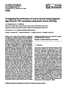
9 Investigating the Performance of Rule-based Models with Increasing Complexity on the Prediction of Trip Generation and Distribution Elke Moons1, Geert Wets and Marc Aerts Hasselt University Belgium 1. Introduction Modelling travel behaviour has always been a major research area in transportation analysis. After the second World War, due to the rapid increase in car ownership and car use in Western Europe and the United States, several models have been developed by transportation planners. In the fifties and sixties, travel was assumed to be the result of four subsequent decisions that were modelled: trip generation, trip distribution, mode choice and the assignment of trips to the road network (Ruiter & Ben-Akiva, 1978). These original tripbased models have been extended to ensuing tour-based models (Daly et al., 1983) and activity-based models (Pendyala et al., 1995; Ben-Akiva & Bowman, 1998; Kitamura & Fujii, 1998; Arentze & Timmermans, 2000; Bhat et al., 2004). In tour-based models, trips are explicitly connected in tours, i.e. chains that start and end at the same home or work base. This is carried out by introducing spatial constraints, hereby dealing with the lack of spatial interrelationship which was so apparent in the traditional four-step trip-based model. In activity-based models, travel demand is derived from the activities that individuals and households need or wish to perform. Decisions with respect to travel are driven by a collection of activities that form an activity diary. Travel should therefore be modelled within the context of the entire agenda, or as a component of the activity scheduling decision. In this way, the relationship between travel and non-travel aspects is taken into account. The reason why people undertake trips is one of the key aspects to be modelled in an activity-based model. However, every working transportation model still exists of at least these original four components of trip generation, distribution, mode choice and assignment. In order to fully understand the structure of a traditional transportation model, we need to elaborate on it some more. As shown in Figure 1, trip generation encompasses both the modelling of production (P) and attraction (A) of trips for a certain region (zone). Production is mainly being modelled at the level of the household, incorporating household characteristics (income, car ownership, household composition, …), features of the zone (land price, degree of urbanization) and accessibility of the zone, whereas attraction is modelled at zone level,
1
Corresponding author (E-mail:
[email protected])
www.intechopen.com
Frontiers in Brain, Vision and AI
168
taking into account employment, land use (for industry, education, services, shopping, etc.) and accessibility (Ortúzar & Willumsen, 2001).
Areal data
Trip Generation (P/A)
Trip-ends
Travel costs derived from network data
Distribution/Mode Choice
OD-matrices
Assignment
Traffic flows
Figure 1. Structure of the traditional trip-based model In the trip distribution step, the produced and attracted trips, that either depart or arrive at a certain zone will be combined, so after the first two steps (generation and distribution), the result is an origin-destination (OD) matrix, where each cell denotes the number of trips going from and to a particular zone. In step three (modal split), these OD-matrices will be split up per mode of transport, and these trips will be assigned to the network in the fourth step, taking into account some generalised network costs. After a short history of transportation models and a description of the structure of the traditional model to understand the notions of trip generation and distribution, this introduction will focus on the different types of activity-based (AB) models, since they have become the standard today and the need of AI techniques within the fastest rising type of AB models (i.e. rule-based models) will be shown. Activity-based models aim at predicting which activities will be conducted where, when, with whom, for how long and the transport mode that was used to arrive at the location of the activity. This sequence of choices immediately shows the usefulness of applying AI techniques, since one of the most important application areas of artificial intelligence is decision making, which clearly happens multiple times a day when a trip is planned. In general, AI can be split up into two broad categories: the symbolic AI that focuses on the development of knowledge-based systems, and the computational AI, which includes neural networks, fuzzy systems and genetic algorithms. In this chapter, we will focus on the latter category of methods, more in specific on the use of induction techniques for prediction. But first, it needs to be shown how induction techniques are applied within AB models.
www.intechopen.com
Investigating the Performance of Rule-based Models with Increasing Complexity on the Prediction of Trip Generation and Distribution
169
Actually, several types of models can be distinguished to build an activity-based travel demand model. They range from constraints-based simulation models to utility-maximising and rule-based (computational process) models. Constraints-based simulation models have their roots in time geography, but they are limited in use, because they lack the necessary mechanisms to predict adjustment behaviour of individuals. Currently, the utility-maximising models based on the logit model (multinomial, nested, mixed, paired combinatory, spatially correlated (Ben-Akiva & Lerman, 1985; Hensher & Greene, 2003; Koppelman & Wen, 2000; Bhat & Guo, 2003 a.o.)) are still the most popular choice, however, because of their flexibility, rule-based systems based on AI algorithms are gaining more and more interest. Examples of utility-maximising models are Starchild (Recker et al., 1986), PCATS (Kitamura & Fujii, 1998) and CEMDAP (Bhat et al., 2004), while AMOS (Pendyala et al., 1995, 1998), FAMOS (Pendyala, 2004) and Albatross (Arentze & Timmermans, 2000, 2005) are examples of rule-based models. Utility-maximising models consider different facets of travel patterns simultaneously, however, the process by which individuals arrive at their choices is not modelled at all. Rulebased models represent an attempt of modelling this scheduling process, hereby disregarding the utility-maximising framework. After all, a lot of researchers have argued that people do not always necessarily arrive at ‘optimal’ choices, but rather use heuristics that may be context dependent. In its most simple form, a rule-based model uses a set of simple IF-THEN rules, that take on the following form: IF (condition = X), THEN (perform action Y). This process of rule induction is similar to the process of parameter estimation in algebraic, econometric models. Although these rule-based models perform very well when induction techniques are used (Wets et al., 2000), they also show some limitations. Most of them are based on a quite complex set of rules. However, already in the Middle Ages, William of Occam's razor (Tornay, 1938) stated that ‘Nunquam ponenda est pluralitas sin necesitate’ meaning that ‘Entities should not be multiplied beyond necessity’. Now it has come to be seen as one of the fundamental tenets of modern science and it is often invoked by learning theorists as a justification for preferring simpler models over more complex ones. However, Domingos (1998) teaches us that it is tricky to interpret Occam's razor in the right way. The interpretation ‘Simplicity is a goal in itself’ is essentially correct, while ‘Simplicity leads to greater accuracy’ is not. Moreover, research in the field of psychology (Gigerenzer et al., 1999; Zellner et al., 2001) shows that there is empirical evidence that simple models, based on fast and frugal heuristics that employ a minimum of time, knowledge and computation, often predict human behaviour very well. Moons et al. (2001) examined the performance of simple classifiers for the transport mode dimension of the Albatross model system. It was discovered that the predictive performance of these simple heuristics was only slightly less than that of a more complex induction algorithm. Moons et al. (2002a, 2002b, 2005) investigated the influence of irrelevant attributes on the performance of the decision tree for the transport mode, the travel party, the activity duration and the location agent of the Albatross model system and it was found that a trimmed decision tree, involving considerable less decision rules, did not result in a significant drop in predictive performance compared to the original larger set of rules that was derived from the activitytravel diaries. Similar techniques have been applied in completely different research domains: marketing (Buckinx et al., 2004), artificial intelligence (Koller & Sahami, 1996; Kohavi et al., 1994), bioinformatics (Zheng et al., 2003), etc. In this chapter, the question `To what extent can this result be generalised in a sequential execution of the full set of nine decision trees that make up the complete Albatross model system?' is inspected.
www.intechopen.com
170
Frontiers in Brain, Vision and AI
For reasons outlined above, it was opted to use several induction techniques with an increasing complexity within a rule-based model. Very simple and more complex decision tree induction algorithms are measured against each other, and the resulting predicted OD matrices are compared to the original matrix to investigate the performance of a sequential execution of these (simple) models. The next Section will discuss the methods that are used to arrive at these simple and complex decision trees, whereas in Section 3 a short introduction to the data is given, together with a discussion on the comparison of the performance of the different methods. In Section 4, the results are presented, while the final Section provides the conclusions and some avenues for future research.
2. Methods First of all, the modelling framework is explained, so that one understands which are the different responses that need to be modelled sequentially. Next, the different methods to determine simple and complex decision are presented. 2.1 Modelling framework Albatross, the most complex fully-operational rule-based model to date, was developed for the Dutch Ministry of Transportation (Arentze and Timmermans, 2000, 2005). This chapter uses the activity-diary data that were collected to determine the rules of the original Albatross system. The activity scheduling process happens sequentially at micro level. Figure 2 provides a schematic representation of the Albatross scheduling model.
Figure 2. Sequential decisions making up the Albatross model
www.intechopen.com
Investigating the Performance of Rule-based Models with Increasing Complexity on the Prediction of Trip Generation and Distribution
171
The activity scheduling agent of Albatross is based on an assumed sequential execution of nine decision trees to predict activity-travel patterns. The model first executes a set of decision rules to predict whether or not a particular activity will be inserted in the schedule. At the same time, the transport mode for the primary work activity is chosen, further referred to as ‘mode for work’. If the activity is added, the travel party and the duration of the activity are determined, based on other sets of rules, before a next activity is considered. The order in which activities are evaluated is pre-defined as: daily shopping, services, non-daily shopping, social and leisure activities. Time constraints are used in this step to determine the feasibility of the chosen activities. Subsequently, in order of priority, a general notion of time of the day (e.g. early morning, around noon, …) is determined for each activity. Based on this, for each activity, a preliminary position is determined in the schedule. Hereafter, trip links (i.e. trip chaining decisions) between activities are considered, which means that when tours are included in the schedule, they are identifiable as sequences of one or more out-of-home activities that start at home and end at home. These trip chaining decisions are not only important for timing activities but also for organising trips into tours. For each tour, a transport mode is then determined. Note that if the activity is the primary work activity, then the transport mode was already chosen, if not, the choice of transport mode is made here in the scheduling process. Finally, the location of each activity is set. Possible interactions between mode and location choices are taken into account by using location information as conditions of mode selection rules. Institutional, spatial and time constraints are adopted in this step to determine which locations are feasible. The predictions for each model are based on a simulation procedure. This involves building an activity pattern for each person-day by successively making a decision on each of the nine choice dimensions. A decision involves selecting a choice alternative based on the predicted probability distribution across alternatives on the choice facet concerned. 2.2 The methods A brief literature review indicates that very simple rules may achieve a surprisingly high accuracy on many data sets. For example, Rendell and Seshu (1990) occasionally remark that many real world data sets have ‘few peaks (often just one)’ and are therefore ‘easy to learn’. Further evidence is provided by studies of pruning methods (e.g. Buntine & Niblett, 1992; Clark & Niblett, 1989; Mingers, 1989), where the accuracy is rarely seen to decrease as pruning becomes more severe. This is even so when the rules are pruned to the extreme, using only one or two variables. The most compelling initial indication that very simple rules often perform well, occurs in Weiss et al. (1990). In four of the five data sets studied, classification rules involving two or fewer attributes outperformed the more complex rules. Therefore, in the next subsections, three induction techniques with an increasing complexity are presented. At first, a very simple classifier, called One R, will be used in order to set up the set of rules for each of the dimensions in the Albatross system. Next, we will discuss a feature selection technique that will applied first to determine the relevant variables before a decision tree is determined. And finally, the C4.5 algorithm to determine a decision tree will shortly be introduced.
www.intechopen.com
Frontiers in Brain, Vision and AI
172
2.2.1 One R Holte developed a very simple classifier that provides a rule based on the value of a single attribute. This algorithm, which he called One R, may compete with state-of-the-art techniques used in the field (Holte, 1993). Like other algorithms, One R takes as input a set of several attributes and a class variable. Its goal is to infer a rule that predicts the class given the values of the attributes. The One R algorithm chooses the most informative single attribute and bases the rule solely on this attribute. Full details can be found in Holte’s paper, but the basic idea is given below. The accuracy is measured by the percentage of correctly classified instances. For each attribute a, form a rule as follows: For each value v from the domain of a, Let c be the most frequent class in the set of instances where a has value v. Add the following clause to the rule for a: If a has value v then the class is c Calculate the classification accuracy of this rule. Use the rule with the highest accuracy. The algorithm assumes that the attributes are discrete. If not, they must be discretised. Any method for turning a range of values into disjoint intervals must take care to avoid creating large numbers of rules with many small intervals. This is known as the problem of ‘overfitting’, because such rules are overly specific to the data set and do not generalise well. Holte achieves this by requiring all intervals (except the rightmost) to contain more than a predefined number of examples in the same class of the outcome variable. Empirical evidence (Holte et al., 1989) led to a value of six for data sets with large number of instances and three for smaller data sets (with less than 50 instances). 2.2.2 Relief-F: a feature selection technique Feature selection strategies are often applied to explore the effect of irrelevant attributes on the performance of classifier systems. A feature selection method ranks all the attributes or conditions (features) in descending order of relevance. This relevance can be measured in several ways, leading to two large subclasses in feature selection methods: the filter and the wrapper approach. The fundamental difference between these approaches is the evaluation criterion used to select or rank attributes. For wrappers, the selection or ranking results from the estimation of the performance on the associated induction algorithm, while the filter approach only makes use of the characteristics of the data itself. Both methods have been compared extensively (Hall, 1999a, 1999b; Koller & Sahami, 1996). In this analysis, the filter approach, more specifically the Relief-F feature selection method is chosen because it can handle multiple classes of the dependent variable (the nine different choice facets that we are predicting range from two to seven classes) and because it can easily be combined with the C4.5 induction algorithm (Quinlan, 1993). Feature selection strategies can be regarded as one way of coping with correlation between attributes. This is relevant because the structure of trees is sensitive to possible multicollinearity, which implies that some variables would be simply redundant (given the presence of other variables). Redundant variables do not affect the impact of the remaining
www.intechopen.com
Investigating the Performance of Rule-based Models with Increasing Complexity on the Prediction of Trip Generation and Distribution
173
variables in the tree model, but it would simply be better if they were not used for splitting. Therefore, a good feature selection method would search for a subset of relevant features that are highly correlated with the class or action variable that the tree-induction algorithm is trying to predict, while mutually having the lowest possible correlations. Relief (Kira & Rendall, 1992), the predecessor of Relief-F, is a distance-based feature weighting algorithm. It orders attributes according to their importance. To each attribute it assigns the initial value of zero that will be adapted with each run through the instances of the dataset. The features with the highest values are considered to be the most relevant, while those with values close to zero or with negative values are judged irrelevant. Thus Relief imposes a ranking on features by assigning each a weight. The weight for a particular feature reflects its relevance in distinguishing the classes. In determining the weights, the concepts of near-hit and near-miss are central. A near-hit of instance i is defined as the instance that is closest to i (based on Euclidean distance) and which is of the same class (concerning the output or action variable), while a near-miss of i is defined as the instance that is closest to i (based on Euclidean distance) and which is of a different class (concerning the output variable). The algorithm attempts to approximate the following difference of probabilities for the weight of a feature X: WX
=
P(different value of X | nearest instance of different class) P(different value of X | nearest instance of same class)
Thus, Relief works by random sampling an instance and locating its nearest neighbour from the same and opposite class. The nearest neighbour is defined in terms of the Euclidean distance. That is, in an n-dimensional space, the following distance measure:
⎞ ⎛ n d( x , y ) = ⎜⎜ ∑ (x i − y i )2 ⎟⎟ , where x and y are two n-dimensional vectors. ⎠ ⎝ i=1 By removing the context sensitivity provided by the ‘nearest instance’ condition, attributes are treated as mutually independent, and the previous equation becomes: 1/2
ReliefX = P(different value of X | different class) P(different value of X | same class). Relief-F (Kononenko, 1994) is an extension of Relief that can handle multiple classes and noise caused by missing values, outliers, etc. To increase the reliability of Relief’s weight estimation, Relief-F finds the k nearest hits and misses for a given instance, where k is a parameter that can be specified by the user. For multiple class problems, Relief-F searches for nearest misses from each different class (with respect to the given instance) and averages their contribution. The average is weighted by the prior probability of each class. 2.2.3 C4.5: a decision tree algorithm Decision tree induction is similar to parameter estimation methods in econometric models. The goal of tree induction is to find the set of Boolean rules that best represents the empirical data. The original Albatross system was derived using a Chi-square based approach. In this study, however, the decision trees were re-induced using the C4.5 method (Quinlan, 1993) because this method is a benchmarking method in the data mining
www.intechopen.com
Frontiers in Brain, Vision and AI
174
community. Wets et al. (2000) found approximately equal performance of these two tree induction algorithms in terms of goodness of fit in a representative case study. The C4.5 algorithm works as follows. Let there be given a set of choice observations i taken from activity-travel diary data. Consider the n different attributes or conditions
X i1 , X i 2 ,..., X in and the choice or action variable Yi ∈ {1,2 ,..., p} for i = 1, … I. In general, a decision tree consists of different layers of nodes. It starts from the root node in the first layer or first parent node. This parent node will split into daughter nodes on the second layer. In turn, each of these daughter nodes can become a new parent node in the next split, and this process may continue with further splits. A leaf node is a node, which has no offspring nodes. Nodes in deeper layers become increasingly more homogeneous. An internal node is split by considering all allowable splits for all variables and the best split is the one with the most homogeneous daughter nodes. The C4.5 algorithm recursively splits the sample space on X into increasingly homogeneous partitions in terms of Y, until the leaf nodes contain only cases from a single class. Increase in homogeneity achieved by a candidate split is measured in terms of an information gain ratio. To understand this concept, the following definitions are relevant: Definition 1: Information of a message The information conveyed by a message depends on its probability and can be measured in bits as minus the logarithm to base 2 of that probability. ̈ For example, if there are four equally probable messages, the information conveyed by any of them is - log2 (1/4) = 2 bits. Definition 2: Information of a message that a random case belongs to a certain class ⎛ freq(C i , T ) ⎞ ⎟ bits − log 2 ⎜⎜ ⎟ T ⎝ ⎠
with T a training set of cases, Ci a class i and freq(Ci, T) the number of cases in T that belongs to class Ci. ̈ Based on these definitions, the average amount of information needed to identify the class of a case in a training set (also called entropy) can be deduced as follows: Definition 3: Entropy of a training set info(T ) = − ∑ k
i=1
⎛ freq(C i , T ) ⎞ freq(C i , T ) ⎟ bits × log 2 ⎜⎜ ⎟ T T ⎠ ⎝
with T a training set of cases, Ci a class i and freq(Ci, T) the number of cases in T that belongs to class Ci. ̈ Entropy can also be measured after that T has been partitioned in n sets using the outcome of a test carried out on attribute X. This yields: Definition 4: Entropy after the training set has been partitioned on a test X info X (T ) =
∑ n
Ti
i =1
T
× info(Ti )
̈
Using these two measurements, the gain criterion can be defined as follows: Definition 5: Gain criterion gain(X) = info(T) - infoX(T) ̈
www.intechopen.com
Investigating the Performance of Rule-based Models with Increasing Complexity on the Prediction of Trip Generation and Distribution
175
The gain criterion measures the information gained by partitioning the training set using the test X. In ID3, the ancestor of C4.5, the test selected is the one which maximizes this information gain because one may expect the remaining subsets in the branches will be the most easy to partition. Note, however, that by no means this is certain because we have looked ahead only one level deep in the tree. The gain criterion has only proved to be a good heuristic. Although the gain criterion performed quite well in practice, the criterion has one serious deficiency, i.e. it tends to favour conditions or attributes with many outcomes. Therefore, in C4.5, a somewhat adapted form of the gain criterion is used. This criterion is called the gain ratio criterion. According to this criterion, the gain attributable to conditions with many outcomes is adjusted using some kind of normalisation. In particular, the split info(X) measure is defined as: Definition 6: Split info of a test X split info(X ) = − ∑ n
Ti
i =1
T
⎛ Ti ⎞ ⎟ × log 2 ⎜ ⎜ T ⎟ ⎝ ⎠
̈
This indicates the information generated by partitioning T into n subsets. Using this measure, the gain ratio is defined as: Definition 7: Gain ratio gain ratio(X) = gain(X) / split info(X) ̈
This ratio represents how much of the gained information is useful for classification. In case of very small values of split info(X) (in case of trivial splits), the ratio will tend to infinity. Therefore, C4.5 will select the condition which maximises the gain ratio, subject to the constraint that the information gain must be at least as large as the average information gain over all possible tests. After building the tree, pruning strategies are adopted. This means that the decision tree is simplified by discarding one or more sub-branches and replacing them with leaves.
3. Model comparison 3.1 The data The analyses are based on the activity diary data used to derive the original Albatross system. The data are collected in February 1997 for a random sample of 1649 respondents in the municipalities of Hendrik-Ido-Ambacht and Zwijndrecht (South Rotterdam region) in the Netherlands. The data consist of full activity-diaries, implying that both inhome and out-of-home activities were reported. Respondents are asked, for each successive activity, to provide information about the nature of the activity, the day, start and end time, the location where the activity took place, the transport mode (chain), the travel time per mode and, if relevant, accompanying individuals. A pre-coded scheme is used for activity reporting. More details can be found in Arentze and Timmermans (2000). A 75-25% split was made on the data set as a whole, where the first 75% are used to build the nine different models, whereas the remaining 25% was left to validate them. 3.2 Model performance Model performance tests are conducted at two levels: the choice facet level, i.e. the level of the separate decision trees and the trip matrix level. Recall that the Albatross system consists
www.intechopen.com
Frontiers in Brain, Vision and AI
176
of nine different choice facets or dimensions and that each of them determines a different response variable. For every dimension, a separate model needs to be built. The strategy for building the C4.5 trees and the trees after feature selection was as follows. The C4.5 trees were induced based on one simple restriction: the final number of cases in a leaf node must meet a minimum of 15, except for the very large data set of the ‘select’-dimension, where this number was set to 30. In the feature selection analysis, all the irrelevant attributes were first removed from the data by means of Relief-F feature selection method with the k parameter set equal to 10. Next, the C4.5 trees were built based on the same restrictions as before, though only the remaining relevant attributes were used. To determine the variable selection, several decision trees were built, each time removing one more irrelevant attribute. For each of these decision trees, the accuracy was calculated and compared to the accuracy of the decision tree of the C4.5 approach. The smallest decision tree, which resulted in a maximum decrease of 2% in accuracy compared to the decision tree including all features, was chosen as the final model for a single choice facet in the feature selection approach. This strategy was applied to all nine dimensions of the Albatross model. At choice facet level, we will compare the number of attributes used to build the decision trees and the obtained accuracy. To have an idea about the complexity of the modelling process, the general statistics for the decision tables for each of the nine dimensions can be found in Table 1. This table describes the statistics on the training set. Dimension
Nr. of cases
Nr. of independent variables
Mode for work (MW)
858
32
Selection (S)
14190
40
With-whom (WW)
2970
39
Duration (D)
2970
41
Start time (ST)
2970
63
Trip chain (TC)
2651
53
Mode other (MO)
2602
35
Location 1 (L1)
2112
28
Location 2 (L2)
1027
28
Table 1. General statistics per dimension At the trip matrix level, the observed and predicted Origin-Destination (OD) matrices are compared. The basic unit for generating an OD-matrix is a trip. It contains the frequency of trips for each combination of origins (rows) and destinations (columns). The Albatross system consists of 20 zones (i.e. origins and destinations) that are used as basis for each ODmatrix. A general OD-matrix is generated, and next to this, it can also be broken down according to a variable like e.g. the transport mode (car driver, slow mode, car passenger, public transport, unknown transport mode), such that different OD-matrices for each mode of transport are obtained (see also Figure 1). Note that the number of cells and hence, the degree of disaggregation, differs between the matrices. For example, the basic OD-matrix has 20x20=400 cells, while the OD-matrix by transport mode has 5x20x20 = 2000 cells. The measure that will be used for determining the degree of correspondence between the observed and predicted matrices is the correlation coefficient. It will be calculated between
www.intechopen.com
Investigating the Performance of Rule-based Models with Increasing Complexity on the Prediction of Trip Generation and Distribution
177
observed and predicted matrix entries in general and for the trip matrices that are disaggregated on transport mode. How can one determine the correlation coefficient between matrices? In both cases, the cells of the OD-matrices are rearranged into a single vector across categories and the correlation coefficient will be calculated by comparing the corresponding elements in the observed and the predicted vector. Thus, for the OD-matrices disaggregated on the transport mode, the cells of the matrices on car driver, slow transport, car passenger, public transport and unknown mode are rearranged into five separate vectors, and these five vectors are combined into one single vector. This occurs for the observed and the predicted matrices, and the correlation coefficient between this observed and predicted vector is the performance measure at trip matrix level. An advantage of the use of the correlation coefficient is that it is insensitive to the difference in scale between column frequencies (i.e. the difference in the total number of trips).
4. Results Note that for reasons of comparison, the results of the Zero R classifier have also been added in this results Section. This Zero R classifier automatically classifies new instances to the majority class. Firstly, we will take a closer look at the average length of the observed and predicted sequences of activities. In the observed patterns, the average number of activities equals 5.160 for the training set and 5.155 for the test set. This average length offers room for 1-3 flexible activities complemented with 2-4 in-home activities. Considerable variation occurs, however, as indicated by the standard deviation of approximately 3 activities. The average length of the predicted patterns for the four modelling approaches is shown in Table 2. Method
Training set
Test set
Zero R
5.217 (3.241)
5.199 (3.333)
One R
5.198 (3.182)
5.178 (3.128)
Feature Selection
5.014 (3.033)
4.907 (2.921)
C4.5
5.286 (2.953)
5.286 (2.937)
Table 2. Average number of predicted activities in the sequences (standard deviation) On average, when comparing the simple classifiers, Zero R and One R overestimate the number of activities, however, this overestimation is somewhat less pronounced on the test set. All models seem to overestimate the variance a little, both on the training set and on the test set. We observe that in general the C4.5 approach predicts activity sequences that are somewhat too long, while those of the feature selection approach are rather a little bit too short. The results of these different methods will now be compared at two other levels, the choice facet level and the trip matrix level. Secondly, the results at the level of each decision tree separately are compared to each other. The models have an increasing complexity in the number of variables that they take into account, but we will also look at the total complexity of the decision tree (i.e. the number of final leaves). Furthermore, the accuracy of the four modelling approaches will also be compared. Table 3 summarises the results.
www.intechopen.com
Frontiers in Brain, Vision and AI
178
Method
Measure
MW
S
WW
D
ST
TC
MO
L1
L2
Zero R
Variables
0
0
0
0
0
0
0
0
0
Leaves
1
1
1
1
1
1
1
1
1
Accuracy
52.5
66.9
35.5
33.4
17.2
53.3
38.8
37.5
20.0
Variables
1
1
1
1
1
1
1
1
1
Leaves
6
5
5
3
4
2
4
3
3
Accuracy
59.5
67.7
40.8
34.8
22.7
69.9
41.3
43.5
23.4
Feature
Variables
2
0
4
4
8
10
11
6
8
Selection
Leaves
6
1
51
38
1
13
60
15
14
Accuracy
59.5
66.9
46.7
36.8
17.2
81.1
50.8
51.3
31.2
Variables
3
15
19
28
28
4
15
8
15
Leaves
8
35
72
148
121
8
63
30
47
Accuracy
59.8
68.6
49.9
43.1
40.8
80.2
52.4
54.0
37.2
One R
C4.5
Table 3. Performance at the level of the decision trees The results show that One R clearly improves on the results of Zero R. Furthermore, the feature selection approach generally generates considerably less complex decision trees than the C4.5 approach. One exception is the ‘trip chaining’ dimension, which has more final leaves in the decision trees with feature selection, when compared to the tree without. Although it is interesting to investigate the results at the level of the decision tree itself, the results are as expected. More complex trees lead to a higher accuracy, although the gain in accuracy is not that high, while much more complexity is required. Therefore, it seems more interesting to look at the result after the whole scheduling process has been carried out and the trips that are predicted are distributed over origins and destinations. Thirdly, the results are compared at trip matrix level, where the observed number of trips from a certain origin to a certain destination is compared to the predicted number of trips, and this for each OD-pair. Correlations are calculated between the final observed and predicted OD-matrices, and also between the OD-matrices that were disaggregated on travel mode, so after step two and step three in the traditional four-step trip-based transportation model. Method
Training data ρ(o,p)
ρ(o,p) mode
Test data ρ(o,p)
ρ(o,p) mode
Zero R
0.938
0.841
0.925
0.787
One R Feature Selection C4.5
0.936
0.880
0.928
0.862
0.957
0.887
0.947
0.849
0.962
0.885
0.942
0.856
Table 4. Model performance at trip matrix level
www.intechopen.com
Investigating the Performance of Rule-based Models with Increasing Complexity on the Prediction of Trip Generation and Distribution
179
Table 4 shows that all correlation coefficients are quite similar. The test set is the most relevant dataset for comparison of the models, so therefore we will focus on this latter one. After the trip distribution step, the feature selection approach shows the highest correlation on the test set. While after the disaggregation of trips according to the different transport modes, the One R approach even shows the highest correlation. This clearly indicates the non-inferior performance of simpler models when compared to the most complex model (C4.5). Table 5 shows the results on the test set more in detail. Mode
Observed
Zero R
One R
Feature sel.
C4.5
Car Slow Public Car passenger
1609 814 79 294
1580 1020 83 356
1609 1013 81 321
1466 920 107 333
1573 1038 113 375
Table 5. Number of trips at trip matrix level: Test set in detail It can be seen that the number of trips undertaken as a car driver is correctly predicted by the One R approach and underestimated by the remaining approaches, while the use of any other transport mode appears to be overestimated. The stability of the different models has also been tested, and the extent to which overfitting may have occurred is approximately the same and at an acceptable level for all models.
5. Conclusions and future research Rule-based models that predict travel behaviour based on activity diary data have been suggested in the literature over the past two decades. These models usually perform very well, though, very often, they are based on a very complex set of rules. Moreover, research in the field of psychology has learned us that simple models often predict human behaviour very well. In fact, the call for simplicity is a question of all ages. Occam's razor, that has to be situated already in the Middle Ages, being an important example. In addition, one has to be careful in interpreting these previous studies, they only support the proposition ‘Simplicity is a goal in itself’, not that simplicity would lead to greater accuracy or better models. It is in this light that this chapter should be regarded. We regarded two ways of simplifying the complex set of rules used to determine the Albatross system. On the one hand, we used two simple classifiers to predict the nine dimensions, while on the other hand we performed two similar analyses: one with and one without irrelevant variables. The results of the tree-induction algorithms can namely be heavily influenced by the inclusion of irrelevant attributes. On the one hand, this may lead to overfitting, while one the other hand, it is not evident whether the inclusion of irrelevant attributes would lead to a substantial loss in accuracy and/or predictive performance. The aim of the study reported in this chapter therefore was to further explore this issue in the context of the Albatross model system, currently the most comprehensive operational computational, rule-based process model of travel demand. The results of the simple classifiers do indicate that the ‘simpler’ models do not perform better, but, on the other hand, it is also not the case that they are inferior to the complex C4.5
www.intechopen.com
180
Frontiers in Brain, Vision and AI
approach. It is rather logical that the model that always takes the majority class (Zero R) does not perform that well, conversely, the models that make up their decisions based on one or a few variables are not in any case second to the complex analysis. This comes as a welcome bonus. The results of the analyses conducted at the two different levels of performance, indicate that, also in the second way of simplification, the simpler models do not necessary perform worse. In fact, more or less the same results were obtained at trip generation level, with or without disaggregating on transport mode. At the choice facet level, one can observe that a strong reduction in the size of the trees as well as in the number of predictors is possible without adversely affecting predictive performance too much. Thus, at least in this study, there is no evidence of substantial loss in predictive power in the sequential use of decision trees to predict activity-travel patterns. The results indicate that using feature selection in a step prior to tree induction can improve the performance of the resulting sequential model. It should be noted, however, that predictive performance and simplicity are not the only criteria. The most important criterion is that the model needs to be responsive to policy sensitive attributes and it needs to be able to model the behavioural mechanisms. For that reason, policy sensitive attributes, such as for example service level of the transport system, or particular behavioural attributes should have a high priority in the selection of attributes if the model is to be used for predicting the impact of policies. The feature selection method allows one to identify and next eliminate correlated factors that prevent the selection of the attributes of interest during the construction of the tree, so that the resulting model will be more robust to policy measures. By these findings, the primary belief that people rely for their choices on some simple heuristics is endorsed. In real life, every person is limited in both knowledge and time and it is infeasible to consider all the different possibilities, before trying to make an optimal choice. Since, in the Albatross system, we are trying to predict nine different choices on travel behaviour made by human beings, this might give an idea on why these simple models do not necessarily perform worse than the complex models. In fact, this is not totally true. If simple models are able to predict the choices of a human being, this can mean two things: either the environment itself is perceived as simple, or the complex choice process can be described by simple models. Since activity-based transport modellers keep developing systems with an increasing complexity in order to try to understand the travel behaviour undertaken by humans, we acknowledge that the environment is not simple. However, whether it is perceived as simple by human beings, remains an open question.
6. References Arentze, T.A. & Timmermans, H.J.P. (2000) Albatross: A Learning-Based Transportation Oriented Simulation System, Eindhoven University of Technology, EIRASS. Arentze, T.A. and H.J.P. Timmermans (2005). Albatross 2: A Learning-Based Transportation Oriented Simulation System, European Institute of Retailing and Services Studies. Eindhoven, The Netherlands. Ben-Akiva, M. & Lerman, S. (1985) Discrete Choice Analysis, M.I.T. Press, Cambridge, MA. Ben-Akiva, M.E. & Bowman, J.L. (1998) Integration of an activity-based model system and a residential location model. Urban Studies, 35(7), pp. 1231-1253.
www.intechopen.com
Investigating the Performance of Rule-based Models with Increasing Complexity on the Prediction of Trip Generation and Distribution
181
Bhat, C.R. & Guo, J. (2003) A mixed spatially correlated Logit model: formulation and application to residential choice modeling. Paper presented at the 82nd Annual Meeting of the Transportation Research Board, Washington, D.C. Bhat, C.R.; Guo, J.; Srinivasan, S. & Sivakumar, A. (2004) Comprehensive econometric microsimulator for daily activity-travel patterns, Electronic proceedings of the 83rd Annual Meeting of the Transportation Research Board, Washington, D.C., USA. Buckinx W.; Moons, E.; Van den Poel, D. & Wets, G. (2004) Customer-adapted coupon targeting using feature selection. Expert Systems with Applications, 26(4), pp. 509-518. Buntine, W. & Niblett, T. (1992) A further comparison of splitting rules for decision-tree induction. Machine Learning, 8, pp. 75--86. Clark, P. & Niblett, T. (1989) The CN2 induction algorithm. Machine Learning, 3, pp. 261-283. Daly, A.J.; van Zwam, H.H. & van der Valk, J. (1983) Application of disaggregate models for a regional transport study in The Netherlands. Paper presented at the 3rd World Conference on Transport Research, Hamburg, Germany. Domingos, P. (1998) Occam's two razors: The sharp and the blunt. Proceedings of the Fourth International Conference on Knowledge Discovery and Data Mining, pp. 37-43. Gigerenzer, G.; Todd, P.M. & the ABC Research Group. (1999) Simple Heuristics That Make Us Smart, Oxford University Press, New York. Hall, M.A. (1999a) Correlation-based Feature Selection for Machine Learning. Ph.D. dissertation, Department of Computer Science, University of Waikato, Hamilton. Hall, M.A. (1999b) Feature selection for machine learning: Comparing a correlation-based filter approach to the wrapper. Proceedings of the Florida Artificial Intelligence Symposium (FLAIRS), Orlando, Florida, USA. Hensher, D. & Greene, W.H. (2003) The mixed logit model: The state of practice, Transportation, 30(2), pp. 133–176. Holte, R.C.; Acker, L. & Porter, B.W. (1989) Concept learning and the problem of small disjuncts. Proceedings of the eleventh international joint conference on artificial intelligence, pp. 813-818, Morgan Kaufmann. Holte, R.C. (1993) Very simple classification rules perform well on most commonly used datasets. Machine Learning, 11, pp. 63-90. Kira, K. and Rendall, L.A. (1992) A practical approach to feature selection. Proceedings of the 9th International Conference on Machine Learning, Aberdeen, Scotland, UK, Sleeman, D.H. & Edwards, P. (eds.), pp. 249-256, Morgan Kaufmann Publishers, San Mateo. Kitamura, R. & Fujii, S. (1998) Two computational process models of activity-travel choice. In: Theoretical Foundations of Travel Choice Modeling, Gärling, T.; Laitila, T. & Westin, K. (eds.), pp. 251—279, Elsevier, Oxford. Kohavi, R., Becker, B. & Sommerfield, D. (1997) Improving simple bayes. Poster papers of the 9th European conference on machine learning, pp. 78-87. Koller, D. & Sahami, M. (1996) Toward optimal feature selection. In: Proceedings of the 13th International Conference on Machine Learning, Saitta, L. (ed.), pp. 284-292, Bari, Italy. Kononenko, I. (1994) Estimating attributes: analysis and extensions of relief. Proceedings of the 7th European Conference on Machine Learning, Catania, Italy, Bergadano, F. & De Raedt, L. (eds.), pp. 171-182, Springer Verlag. Koppelman, F. & Wen, C-H. (2000) The Paired Combinatorial Logit model: Properties, estimation and application. Transportation Research B, 34(2), pp. 75-89.
www.intechopen.com
182
Frontiers in Brain, Vision and AI
Mingers, J. (1989) An empirical comparison of pruning methods for decision tree induction. Machine Learning, 4(2), pp. 227-243. Moons, E.; Wets, G.; Vanhoof, K.; Aerts, M. & Timmermans, H. (2001) How well perform simple rules on activity diary data. Proceedings of the 7th International Computers in Urban Planning and Urban Management Conference, Honolulu, USA. Moons, E.; Wets, G.; Aerts, M. & Vanhoof, K. (2002a) The role of Occam's razor in activity based modeling. In: Computational Intelligent Systems for Applied Research Proceedings of the 5th International FLINS Conference, Ruan, D., D'hondt, P. and Kerre, E.E. (Eds.), pp. 153-162, Gent, Belgium. Moons, E.; Wets, G.; Vanhoof, K.; Aerts, M.; Arentze, T. & Timmermans, H. (2002b) The impact of irrelevant attributes on the performance of classifier systems in generating activity schedules. Proceedings of the 81st Annual Meeting of the Transportation Research Board, Washington D.C., USA. Moons, E.A.L.M.G.; Wets, G.P.M.; Aerts, M.; Arentze, T.A. & Timmermans, H.J.P. (2005) The impact of simplification in a sequential rule-based model of activity scheduling behavior. Environment and Planning A, 37(3), pp. 551-568. Ortúzar, J. de D. & Willumsen, L.G. (2001). Modelling Transport (3rd ed.), Wiley. Pendyala, R.M.; Kitamura, R. & Reddy, D.V.G.P. (1995) A rule-based activity-travel scheduling algorithm integrating neural networks of behavioral adaptation. Paper presented at the EIRASS Conference on Activity-Based Approaches, Eindhoven, The Netherlands. Pendyala, R.M.; Kitamura, R. & Reddy, D.V.G.P. (1998) Application of an activity-based travel demand model incorporating a rule-based algorithm. Environment and Planning B, 25, pp. 753-772. Pendyala, R.M. (2004) FAMOS: Application in Florida. Paper presented at the 83rd Annual Meeting of the Transportation Research Board, Washington, D.C., USA. Quinlan, J.R. (1993) C4.5 Programs for Machine Learning, Morgan Kaufmann Publishers, San Mateo. Recker, W.W.; McNally, M.G. & Root, G.S. (1986) A model of complex travel behavior: Part 2: an operational model. Transportation Research A, 20, pp. 319-330. Rendell, L. & Seshu, R. (1990) Learning hard concepts through constructive induction. Computational Intelligence, 6, pp. 247-270. Ruiter, E.R. & Ben-Akiva, M. (1978) Disaggregate travel demand models for the San Francisco bay area. Transportation Research Record, 673, pp. 121-128. Tornay S. (1938) Ockham: Studies and Selections, La Salle, IL: Open Court. Weiss, S.M.; Galen, R.S. & Tadepalli, P.V. (1990) Maximizing the predictive value of production rules. Artificial Intelligence, 45, pp. 47-71. Wets, G., Vanhoof, K., Arentze, T. and Timmermans, H. (2000) Identifying decision structures underlying activity patterns: an exploration of data mining algorithms. Transportation Research Record, 1718, pp. 1-9. Zheng, C.L.; de Sa, V.R.; Gribskov, M. & Murlidharan Nair, T. (2003) On selecting features from splice junctions: an analysis using information theoretic and machine learning approaches, Genome Informatics, 14, pp. 73--83. Zellner, A.; Keuzenkamp, H.A. & McAleer, M. (2001). Simplicity, Inference and Modelling: Keeping It Sophisticatedly Simple, Cambridge University Press, Cambridge, United Kingdom.
www.intechopen.com
Brain, Vision and AI
Edited by Cesare Rossi
ISBN 978-953-7619-04-6 Hard cover, 284 pages Publisher InTech
Published online 01, August, 2008
Published in print edition August, 2008 The aim of this book is to provide new ideas, original results and practical experiences regarding service robotics. This book provides only a small example of this research activity, but it covers a great deal of what has been done in the field recently. Furthermore, it works as a valuable resource for researchers interested in this field.
How to reference
In order to correctly reference this scholarly work, feel free to copy and paste the following: Elke Moons, Geert Wets and Marc Aerts (2008). Investigating the Performance of Rule-based Models with Increasing Complexity on the Prediction of Trip Generation and Distribution, Brain, Vision and AI, Cesare Rossi (Ed.), ISBN: 978-953-7619-04-6, InTech, Available from: http://www.intechopen.com/books/brain_vision_and_ai/investigating_the_performance_of_rulebased_models_with_increasing_complexity_on_the_prediction_of_t
InTech Europe
University Campus STeP Ri Slavka Krautzeka 83/A 51000 Rijeka, Croatia Phone: +385 (51) 770 447 Fax: +385 (51) 686 166 www.intechopen.com
InTech China
Unit 405, Office Block, Hotel Equatorial Shanghai No.65, Yan An Road (West), Shanghai, 200040, China Phone: +86-21-62489820 Fax: +86-21-62489821