´Arpád Maróti, Dávid Szalóki, Domokos Kiss, Gábor Tevesz. Department of Automation and Applied Informatics,. Budapest University of Technology And ...
SAMI 2013 • IEEE 11th International Symposium on Applied Machine Intelligence and Informatics • January 31 - February 2, 2013 • Herl’any, Slovakia
Investigation of Dynamic Window Based Navigation Algorithms on a Real Robot ´ ad Mar´oti, D´avid Szal´oki, Domokos Kiss, G´abor Tevesz Arp´ Department of Automation and Applied Informatics, Budapest University of Technology And Economics, H-1117 Budapest, Magyar Tud´osok k¨or´utja 2., Hungary {Maroti.Arpad, Szaloki.David, Kiss.Domokos, Tevesz.Gabor}@aut.bme.hu
the idea of Dynamic Window Approach. Section III describes our environment and robot model, and then the collision checking method is being discussed. In Section IV a solution for avoiding trap situations is introduced. Simulation and real test results are being presented and summarized in Section V. Our future tasks, and yet unresolved problems are discussed in Section VI.
Abstract—The Dynamic Window Approach (DWA) to collision avoidance is a well-known and elegant method in the mobile robotics field. It provides a collision-free navigation between obstacles, and takes the dynamic properties of the robot into account. Numerous variants had been proposed for this approach, most of them are using an objective function consisting of weighted terms. The solution named Global Dynamic Window Approach with Receding Horizon Control (GDWA/RHC) uses a global navigation function — which is a scalar-valued function representing the distance from the goal point — as the objective function. In this paper, a real-world implementation of the DWA and the GDWA/RHC methods is introduced.
II. BACKGROUNDS AND RELATED WORK The former approaches used potential fields [3] and virtual forces [4], in order to push the robot away from the obstacles, and pull it to the goal position. The Dynamic Window Approach of robot navigation differs from them, in that it takes the kinematic and dynamic constraints of the robot into account using a velocity motion model. This method assumes that the trajectories of the robot can be approximated by a sequence of circular arcs. For every circle segment, a velocity pair (v, ω) can be assigned, where v is the translational and ω is the angular velocity of the robot. The velocity space consists of the achievable velocity pairs for the robot. This approach takes the dynamic constraints of the robot into account by limiting the search space to the velocities that can be reached in a short time interval. This range of the velocity space is the dynamic window, thus the name of the approach. A velocity inside the dynamic window is considered safe if the robot can travel following its corresponding curvature for one cycle and then stop without collision. Since the velocity space is continuous, the range of the dynamic window has to be sampled, and the selected velocities have to be tested for safety. Those, which are considered safe, are called admissible velocities. To choose from the list of admissible velocities an objective function is evaluated and maximized. This function is a weighted sum of three terms:
I. I NTRODUCTION Motion planning is one of the most elemental problems in the field of mobile robotics. Autonomous mobile robots should be able to find a path to the goal position, and the collision-less navigation is crucial. This problem had been discussed in many studies, and numerous methods had been developed in the last decades. These can be grouped into two basic categories. The global planning methods use a priori information of the workspace, while the local methods (also known as reactive methods) rely on only close environmental data. Although, the global navigation algorithms are usually able to find the optimal path to the destination, they usually require massive computational capacity, which increases radically in non-static environments. Local solutions deal with less data and require less computing, thus they are more suitable for real-time application in autonomous mobile robots with limited processing performance. Besides, they are able to handle changes in their environment. Their main drawback is that in the most cases they cannot guarantee that the robot will actually reach the goal position; it can get stuck in local minima. This paper focuses on our real-world implementation of the Dynamic Window Approach (DWA) [1], and the Global Dynamic Window Approach with Receding Horizon Control (GDWA/RHC) [2]. These are basically reactive methods, but the GDWA/RHC uses global information about free space connectivity in order to eliminate the local minima issue. Since our aim was to create an efficient solution, some calculation speed improvements of the original DWA are introduced here, such as radial sampling of the dynamic window. The organization of this paper is as follows. At first, we give a short survey of collision avoidance methods based on
978-1-4673-5929-0/13/$31.00 ©2013 IEEE
G(v, ω) = σ(α · heading(v, ω) +β · dist(v, ω) +γ · velocity(v, ω))
(1)
where heading(v, ω) is a measure of going into the direction of the goal, dist(v, ω) is the distance that could be travelled along the curvature without any collision, and velocity(v, ω) favours the velocities with high translational speeds.
95
Á. Maróti et al. • Investigation of Dynamic Window Based Navigation Algorithms on a Real Robot
Experimental results [1] indicated that this approach is able to control the robot along a fast and safe path when using proper weighting factors. However, there is no way to determine them algorithmically. Another issue is that the (sub)optimal values depend on the obstacle configuration of the environment, although it is possible to find a set of weighting factors suitable in a wide range of environments. Since DWA is a local navigation algorithm, it is vulnerable to trap situations; there is absolutely no guarantee that it can find a path leading to the goal position. Brock and Khatib [5] introduced the Global Dynamic Window Approach (GDWA) for round-shaped holonomic robots in order to eliminate the previously mentioned local minima problem. It is reached by defining a navigation function (NF) taking the free space connectivity into account. The navigation function is a scalar valued two dimensional grid-based function spreaded across the workspace of the robot, having a uniqe minimum at the goal position. The objective function have been changed to the following form: Ωg (p, v, a) = α · nf 1(p, v) +β · vel(v) +γ · goal(p, v) +δ · ∆nf 1(p, v, a)
navigation methods. The Global Dynamic Window Approach with Receding Horizon Control [2] algorithm works with a non-holonomic circular robot model. It is a modification of [6] using an objective function which has no weighted terms. It is evaluated as follows: u(·) = arg min NF(rx (t + T ), ry (t + T ))
(3)
u(·)
where the function NF returns the value of the navigation function at rx (t + T ) and ry (t + T ), which are the predicted coordinates of the robot at the end of the time horizon. In [9] an improved version of the previous algorithm have been introduced, which takes the robot shape into account and able to operate with holonomic and a class of non-holonomic robot models as well. The contribution of this paper is two dynamic window based implementation of obstacle avoidance on a real robot. The first is a GDWA variant taking the robot shape into account, while the second uses the GDWA/RHC method. Our implementation runs on a robot [10] built at our university for the Eurobot contest [11]. Due to the limited computation performance of the onboard computer of the robot, beside the proper functioning, we had to focus on the calculation efficiency too. Two performance improvement solutions are introduced here as the three-step collision-checking algorithm, and the radial sampling of the velocity space.
(2)
p is the current position, v is the desired speed and a is the desired acceleration. Function nf 1(p, v) favours the velocities aligned to the gradient of the navigation function, vel(v) prefers velocities with higher translational speeds. The goal(p, v) function is a binary function with a value of 1, if the trajectory passes through the goal position and 0 otherwise. The value of ∆nf 1(p, v, a) indicates that how much the value of the navigation function is expected to decrease along the trajectory. This approach eliminates the local minima problem in most ¨ cases, although Ogren and Leonard [6] proved that limit cycles can still evolve when the velociy term outweights the effect of the navigation function terms. In their solution, they reformulated the Dynamic Window Approach as a model predictive control problem (also referred as receding horizon control, RHC) and used the navigation function in their cost function. However, this solution can fail to converge to the goal position and stop far from it, because zero velocity is allowed. The previously mentioned methods have worked with circular or point-like robot model. The circle-shaped robots can be treated as single points, if the obstacles are expanded by the radius of the robot. This assumption makes the collisionchecking algorithm very simple, but it is only advisable if the shape of the robot is approximately circular. Otherwise, if the shape significantly differs from a circle, this assumption may result in false behaviour, since finding narrow passages is not guaranteed. Numerous solutions were published taking the shape of the robot into account, such as [7] and [8]. The authors of the present paper already introduced some
III. G EOMETRICAL REPRESENTATION By the dimensions of the playing area at the Eurobot contest, the configuration space is a 2 meters wide and 3 meters long rectangle. The obstacle configuration is also pre-known. Although the obstacles are mostly static, there are two teams competing at the same time, thus at least one moving opponent is located on the table. In the following subsections, first our environment and robot model, then our collision-checking algorithm is being detailed. A. Environment model In our environment model, obstacles are represented as polygons. Non-polygonal obstacles are approximated by circumscribed polygons. In order to avoid further complications, concave polygons are splitted into a group of convex ones using the Keil-Snoeyink algorithm [12]. For every obstacle an expanded shape is calculated, which contains the points that are not farther from the original obstacle, than the radius of the circumcircle of the robot. These objects are constructed from line segments and circles and being utilized by the collision-checking algorithm. Circumscribed polygons for these expanded objects can also be calculated, and these are necessary for the tangent graph, which is used for the path planning described in Section V. A bounding rectangle with horizontal and vertical sides is also calculated for every expanded shape. These are also used by our collision-checking method. The borders of the playing area are bounded by four obstacles ensuring that the robot cannot leave the table.
96
SAMI 2013 • IEEE 11th International Symposium on Applied Machine Intelligence and Informatics • January 31 - February 2, 2013 • Herl’any, Slovakia
B. Robot model In our robot representation, the robot can have several shapes, and it can be changed on the fly. This can happen for example, when the robot moves it’s arm. When this situation occurs, the expanded shapes, their circumscribed polygons and bounding rectangles have to be recalculated. Our robot has differential drive, thus our model describes a non-holonomic robot. Maximum velocities and maximum acceleration values are stored for each driving motor. Knowing the distance between the two wheels (W ), the current translational (v) and angular (ω) velocities can be calculated as follows: vr + vl 2 (4) vr − vl ω= W where vl and vr are the velocity of the left and the right wheel respectively. In our model, the center of the robot is the midpoint of the common axis of the wheels, which is the fulcrum. A circumcircle with center at the fulcrum is also stored, it’s radius is used for obstacle expansion. v=
Fig. 1.
Collision-checking in the simulator
direction, and calculates that minimal angle, at which the vertex and one of the line segments of the robot has an intersection. The result of the sub-steps are a list of angles, and the smallest is the maximum angle that can be travelled without collision. The output of this third step is the distance, which is calculated from this maximum angle and the radius of the given arc. Fig. 1 is a simulated example, which shows how our collision-checking algorithm works. The dark green shapes are the actual obstacles. Note, that the concave obstacle is splitted into three convex obstacles. Their expanded shapes are the light green rounded shapes, and their bounding rectangles are drawn with even lighter green colour. The polygon of our robot is shown as a blue shape. It’s containing circle, it’s orientation and it’s wheels are also shown. The given arc is displayed with black colour. The bluish rectangles are the bounding rectangles of the obstacles selected for further examination in the first step of our algorithm. The second step selects the circles and the line segments of the expanded shapes of the selected obstacles, which are intersected by the given arc. These are indicated with yellow highlighting. After that, a list of the sides of the original obstacles can be determined and given to the third step. These sides are drawn using yellow colour. The last step of our algorithm determines the maximum distance that can be travelled along the given arc without collision, thus the position of the robot at the moment of the first collision has been displayed.
C. Collision-checking algorithm We developed a three-step collision-checking method, which calculates the distance that can be travelled without collision along a given arc. Our goal was to create a fast and accurate algorithm. The algorithm has three steps, and every step is more complicated than the previous ones. So the preceding calculations filter the input of the following steps. 1) The first step drops obstacles those bounding rectangle does not have any intersection with the given arc. A list of the remaining obstacles are forwarded to the next step. This is a very simple calculation, and filters out the obstacles which are far from the path of the robot. 2) The second step examines every circle and line segment of the expanded shapes, and drops those that do not have any intersection with the given arc. After that, it looks up the expanding source for the remaining ones. In case of a circle the source consists of two line segments from the original obstacle, those have an endpoint at the center of the circle. A list of these line segments are forwarded to the next step. 3) The last step is the most complicated, because this is where the shape of the robot is taken into account. At first, it calculates the central angle of the given arc. After that, the goal is to determine the maximal angle less than the central angle, that the robot can travel without collision along the given arc. This calculation has two sub-steps. The first one rotates every vertices of the shape of the robot around the center of the given arc, and calculates that minimal angle, at which the vertex and one of the given line segments has an intersection. The second substep rotates every endpoints of the given line segments around the center of the given arc in the opposite
IV. W ORKING WITHIN THE VELOCITY SPACE In Section III. it had been introduced, that how our solution determines the maximum distance that can be travelled along a given arc. Our next task is to select these arcs, examine them, than choose from them. In our robot model the tavelling curvature is determined by the speed of the two wheels. Thus, compared to the original
97
Á. Maróti et al. • Investigation of Dynamic Window Based Navigation Algorithms on a Real Robot
representation of velocity space [1] that used the translational and angular velocities, our solution uses the peripheral speed of the wheels as the axes of the coordinate system. This comes handy, because these two variables are independent, so our search space and our dynamic window are square shaped. A. Sampling of the dynamic window From the current speed, and the maximum acceleration of the wheels the actual dynamic window can be calculated. The next problem, which is being discussed here is the sampling of the dynamic window. The most simple solution is the grid-based sampling. Among the constraints of the dynamic window, the velocity space is being sampled at the points of a point grid. For each selected velocity, an arc is determined as follows. W vr + vl v = ω 2 vr − vl s = v · T + stopdistance(v)
R=
Fig. 2.
Radial sampling pattern
(5) The advantage of the radial sampling method is that multiple admissable velocities can be gathered by one collisionchecking calculation. Thus, averagely less computation per sampled velocity point is required. Although, in case of running out of time this solution leaves large unsampled areas, such as the simple method. It can be a solution for the remaining unsampled area issue, if the dynamic window is sampled stochastically for a given time. Note, that this is only applicable when the number of the selected points is large enough, otherwise we probably get a non-even sampling pattern. The stochastical sampling can be applied as well as for the simple, like the radial sampling method. These patterns are displayed in Fig. 3.
where R is the radius and s is the length of the arc. Note, that both value can be positive or negative too, this determines the location and the orientation of the arc. T is the cycle time of the dynamic window algorithm, and stopdistance(v) is the minimal breaking distance along this arc from the given velocity. Each arc is being checked by our collision-check algoritm, and the colliding ones are being filtered out. The advantage of this solution is the simplicity, but it has a disadvantage too. When the calculation takes more time then T , and it has to be interrupted, a large connected area is being left unsampled, which is undesirable. Our newly introduced sampling solution is called radial sampling. Our starting point was, that the robot can travel along the same curvature with different speeds. Thus, if we determine the largest safe velocity along a curvature, every slower translational speed is admissable. In our velocity space representation the arcs with the same curvature are located on half-lines with an endpoint at the origin. We select those sides of the dynamic window, which has a point that can be connected with the origin by a line segment, that goes through the area of the dynamic window. Our method takes velocities along these sides with equal distance, and calculates the maximum distance for every sample that can be travelled without collision. Then, the maximum speed along the curvature is being determined for this distance. If that velocity is inside the dynamic window, it is admissable, and every slower speed with the same curvature — which are located along a half-line with an endpoint at the origin — inside the dynamic window is admissable too. Thus, we sample the half-lines starting from the maximum-speed points with equal distances, until the edge of the dynamic window, or the origin is achieved. The pattern of the radial sampling method is displayed in Fig. 2, where the pink square is the search space, the green one is the dynamic window and the blue points are the examined velocities.
B. Ranking of the admissable velocities The admissable velocities have to be ranked in order to select the one, which leads the robot on the best path to the destination. In our project we implemented two methods. The first is the original DWA objective funtcion (see (1)), and the second one is the GDWA/RHC method (see (3)). The navigation function required by the GDWA/RHC method is calculated according to the description in [2]. After the best velocity is selected, the corresponding wheel speeds are transmitted to the motor drive controllers.
Fig. 3.
98
Stochastical sampling patterns for simple and radial methods
SAMI 2013 • IEEE 11th International Symposium on Applied Machine Intelligence and Informatics • January 31 - February 2, 2013 • Herl’any, Slovakia
Fig. 4.
Fig. 5.
Simulated trajectory of the robot
Fig. 6.
Real-life trajectory of the robot
Finding path in the tangent graph
V. AVOIDING TRAP SITUATIONS Since the DWA method has the local minima problem, we used global information for planning a path travelable by the robot without getting into local minima. The gobal information we use is a tangent graph built on the expanded polygons of the obstacles. The nodes of this graph are those vertices of the expanded polygons, which are not inside of an other expanded polygon. The edges of the tangent graph can be grouped into two types. The first set contains those edges of the expanded polygons, which do not intersect and are not surrounded by any expanded polygon. The second group contains edges, which comply with the following criteria: • They endpoints belong to different expanded polygons • They do not intersect any expanded polygon • Their prolonged lines do not intersect any of the two parent expanded polygons We add the position of the robot and the destination to the nodes. After that all the edges being inserted, which has at least one endpoint at these new nodes, and do not intersect any expanded polygon. On this graph the shortest path from the robot to the destination can easily aquired using Dijkstra’s algoritm, as it is shown in Fig. 4. In case of using DWA ranking, giving the location of the nodes in the path one by one to the robot as the actual destination point, the local minima problem disappears. This path can be useful when the navigation function of the GDWA/RHC method is being calculated. The calculation of the Navigation Fuction can be done only near this path, not for the entire configuration space, thus we can improve the performance of the algorithm.
collision-checking algorithm, and our sampling and ranking methods. The previously presented figures were generated using this tool. Our team was able to simulate the movements of the robot with various sampling and ranking configurations. Fig. 5 shows an example result of the simulation, where the robot navigated in an environment with four rectangular obstacles. During this test, radial sampling and the objective function of the DWA were used. The trajectory of the robot is shown in purple colour. After the simulated tests became successful, the algorithm had been ported to the on-board computer of the robot. We developed our navigation algorithm using native C++ programming language, thus the porting procedure from a Windows-based PC to the Linux-based embedded computer of the robot was quite simple. Note that, when we tested the algorithm using the simulator, the position of the robot was calculated and not measured. In real-life, our robot measures the position using deadreckoning, which has an integral error. Besides that behaviour, it has finite resolution significantly lower than the resolution of our simulator.
VI. S IMULATION AND TEST RESULTS A simulator tool has been created, for supporting the development of the project. It has been used for debugging the
99
Á. Maróti et al. • Investigation of Dynamic Window Based Navigation Algorithms on a Real Robot
Caused by this behaviour, it is often occured during the tests when the robot was close to an obstacle, that the dead-reckoning measurement of the position reported, it is intersecting the obstacle. This confused our collision-checking algorithm and it resulted that the robot was unable to leave the area of the obstacle. We had to slightly change this algorithm to make it handle these situations. In our simulated environment, the robot achieved instantly the velocity prescribed by the algorithm. (This approximation is allowed by the DWA.) In real-life, the reaching of the given velocity is delayed. In practical applications it can be useful, if the moving direction of the robot can be predefined. For example, when the robot has to move something by pushing it in front of itself, it must be defined that the robot is not allowed to move backwards. Hence, we implemented this feature. Fig. 6 shows the trajectory of the robot during a real-life test. The starting position and the destination is the same as in the simulated case (Fig. 5), and the settings of the algorithm are the same too. We noticed that the two trajectories are slightly different. In real tests, the robot usually chooses more sinuous paths, but the reason of this behaviour is not found yet. Our tests showed differencies between the behaviour of the two implemented ranking solutions. The objective function of the DWA usually makes the robot turn into the direction of the destination first, then accelerates towards it. When using the GDWA/RHC method, the robot never rotates in place, it has to have translational velocity in order to change the replacement value of the navigation function. When the robot is located in a narrow passage, and it is not heading to the direction of the passage, it has difficulties in reaching the destination. This issue can be resolved by turning the robot into direction first and starting the algoritm only after that. VII. C ONCLUSIONS AND FUTURE WORK It is proved that the three step collision-checking algorithm is effective enough, so it can be used on processor cards with lower computing performance. It is confirmed that our implemented solutions are functional and in our opinion they may be applicable at the Eurobot contest. Although in order to participate successfully at the competition some future work is required. Our main task is to lower the differences between the simulated and the real-life behavior. It may be achieved by improving the robot model.
In our current tests the maximum translational velocity of the mm robot was 400 mm s . The drive is capable of 1200 s , thus after eliminating the inaccuracy, the speed of the robot can be increased. Handling of opponent robots is already implemented, but we have not tested it yet. The future tests can contain such configurations, in which the robot reconfigures it’s shape, for example by opening an arm. ACKNOWLEDGMENT The work in the paper has been developed in the framework of the project ”Talent care and cultivation in the scientific workshops of BME”. This project is supported by the grant ´ TAMOP - 4.2.2.B-10/1–2010-0009. R EFERENCES [1] D. Fox, W. Burgard, and S. Thrun, ”The dynamic window approach to collision avoidance”, in IEEE Robot. Autom. Mag., vol. 4, pp. 23 33, 1997. [2] D. Kiss and G. Tevesz, ”A receding horizon control approach to navigation in virtual corridors”, in Applied Computational Intelligence in Engineering and Information Technology, ser. Topics in Intelligent Engineering and Informatics. Springer-Verlag, 2012, vol. 1, pp. 175186. [3] O. Khatib, ”Real-time obstacle avoidance for robot manipulator and mobile robots”, in The International Journal of Robotics Research, vol. 5, pp. 9098, 1986. [4] J. Borenstein and Y. Koren, ”The vector field histogram - fast obstacle avoidance for mobile robots”, in IEEE Trans. Robot. Autom., vol. 7, pp. 278288, 1991. [5] O. Brock and O. Khatib, ”High-speed navigation using the global dynamic window approach”, in Proceedings of the IEEE International Conference on Robotics and Automation, Detroit, MI, 1999, pp. 341346. [6] P. Ogren and N. E. Leonard, ”A convergent dynamic window approach to obstacle avoidance”, in IEEE Trans. Robot., vol. 21, pp. 188195, 2005. [7] C. Schegel, ”Fast local obstacle avoidance under kinematic and dynamic constraints for a mobile robot”, in Proceedings of the IEEE/RSJ International Conference on Intelligent Robots and Systems, Victoria, B.C., Canada, 1998, pp. 594599. [8] K. Arras, J. Persson, N. Tomatis, and R. Siegwart, ”Real-time obstacle avoidance for polygonal robots with a reduced dynamic window”, in Proceedings of the IEEE International Conference on Robotics and Automation, Washington, DC, 2002, pp. 30503055. [9] D. Kiss and G. Tevesz, ”Advanced Dynamic Window based Navigation Approach using Model Predictive Control”, in 17th International Conference on Methods and Models in Automation and Robotics, Miedzyzdroje, Poland, 2012, pp. 148-153. [10] D. Varga, K. Csorba, D. Szal´oki, Z. Beck, G. Tevesz, ”Educational aspects of designing robot for Eurobot contest”, in 9th IFAC Symposium on Advances in Control Education (ACE2012), Nizhniy Novgorod, Russia, 2012, pp. 342-347. [11] Eurobot, international robotics contenst, http:// www.eurobot.org [12] M. Keil and J. Snoeyink, ”On the time bound for convex decomposition of simple polygons”, in School of Computer Science, pp. 54-55, 1998.
100