INVESTIGATION ON OPTIMIZATION OF PROCESS PARAMETERS AND CHEMICAL REACTOR GEOMETRY BY EVOLUTIONARY ALGORITHMS Tran Trong Dao Ivan Zelinka Department of Applied Informatics, Tomas Bata University Nad Stranemi 4511, Zlin 760 05, Czech Republic E-mail: {trantrongdao, zelinka}@fai.utb.cz
KEYWORDS Simulation; Optimization; Evolutionary algorithms; Differential evolution; Self-organizing migrating algorithm. ABSTRACT The present work aims to employ evolutionary algorithms (EAs) to optimize an industrial chemical process. A unique combination of the simplified fundamental theory and direct hands-on computer simulation is used to present the modeling of a dynamic chemical engineering process in a highly understandable way. The main aim is to use them for analysis of dynamical system behaviour, especially of a given chemical reactor. A non-linear mathematical model is required to describe the dynamic behaviour of batch process; this justifies the use of evolutionary method of the EAs to deal with this process. Two algorithms - differential evolution and self-organizing migrating algorithm are used in this investigation. Differential Evolution is an evolutionary optimization technique which is exceptionally simple, significantly faster & robust at numerical optimization and is more likely to find a function’s true global optimum. SOMA is also robust algorithm in sense of global extreme searching. In this way, in order to optimize the process, the EAs code is coupled with the rigorous model of the reactor. Both algorithms (SOMA, DE) have been applied 100 times in order to find the optimum of process parameters and the reactor geometry. The results show that the EAs are used successfully in the process optimization. INTRODUCTION Evolutionary algorithms derived by observing the process of biological evolution in nature, have proven to be a powerful and robust optimizing technique in many cases (Gross B.; Roosen P. 1998). In computer science evolutionary computation is a subfield of artificial intelligence (more particularly computational intelligence) that involves combinatorial optimization problems (Wikipedia encyclopedia). Since the 60s, several approaches (genetic algorithms, evolution strategies etc.) have been developed which apply evolutionary concepts for simulation and Proceedings 23rd European Conference on Modelling and Simulation ©ECMS Javier Otamendi, Andrzej Bargiela, José Luis Montes, Luis Miguel Doncel Pedrera (Editors) ISBN: 978-0-9553018-8-9 / ISBN: 978-0-9553018-9-6 (CD)
optimization purposes. Also in the area of multiobjective programming, such approaches (mainly genetic algorithms) have already been used (Evolutionary Computation 3(1), 1–16)(Thomas Hanne 2000). Evolutionary algorithms such as evolution strategies and genetic algorithms have become the method of choice for optimization problems that are too complex to be solved using deterministic techniques such as linear programming or gradient (Jacobian) methods. The large number of applications (Beasley (1997)) and the continuously growing interest in this field are due to several advantages of EAs compared to gradient based methods for complex problems ( Ivo F. Sbalzarini, Sibylle Muller and Petros Koumoutsakos, 2000). The optimization of dynamic process has received growing attention in recent years because it is essential for the process industry to strive for more efficient and agile manufacturing in face of saturated market and global competition (T. Backx, O. Bosgra 2000). In chemical engineering, evolutionary optimization has been applied by the author and others to system identification (Pham and Coulter, 1995; Moros, 1996); a model of a process is built and its numerical parameters are found by error minimization against experimental data. Evolutionary optimization has been widely applied to the evolution of neural networks models for use in control applications (e.g. Li & Haubler, 1996). In this paper, the methods of artificial intelligence by evolutionary algorithms - SOMA and DE are presented for optimizing chemical engineering processes, particularly those in which the evolutionary algorithm is used for static optimization of a chemical batch reactor to improve its parameter. Consequently, it is used to design geometry technique equipments for chemical reaction. The method was used to optimize the design of the growth chamber, and was found to be in good agreement with the observed growth rate results. The area of reactor network synthesis currently enjoys a proliferation of contributions in which researchers from various perspectives are making efforts to develop systematic optimization tools to improve the performance of chemical reactors. The contributions reflect on the increasing awareness that textbook knowledge and heuristics (Levenspiel, 1962), commonly employed in the development of chemical
reactors, are now deemed responsible for the lack of innovation, quality, and efficiency that characterizes many industrial designs. From an economic viewpoint, final-product of the required quality demands a certain respectable maximal productivity of a chemical reactor. The reactor productivity depends on reaction rate, which usually increases exponentially with rising temperature.
inside the reactor with Reactionary mixture then temperature T , specific heat chemicals FK described by a FK .
parameter mass m P . has total mass m , c R and stirs till the time parameter concentration
Non-linear model of reactor Description of the reactor applies a system of four balance equations (1). The first one expresses a mass balance of reaction mixture inside the reactor, the second a mass balance of the chemical FK, and the last two formulate entalpic balances, namely balances of reaction mixture and cooling medium. Equations (1), where for simplified notation of basic equations (2) is represented by term “k”.
m& FK = m′[t ] Figure 1: Batch reactor with single external cooling jacket DESCRIPTION OF A REACTOR This work uses a mathematical model of a reactor shown in Figureure. 2. From constructional standpoint, the acts about the vessel with double side for cooling medium and is further equipped with stirrer for mixing reactionary mixtures.
m& FK = m[t ]a′FK [t ] + k m[t ]aFK [t ]
m& FK cFK TFK + ΔH r k m[t ]aFK [t ] = = K S (T [t ] − TV [t ]) + m[t ]cR T ′[t ]
(1)
m& V cV TVP + K S (T [t ] − TV [t ]) = m& V cV TV [t ] + mVR cV TV′ [t ] k = Ae
−
E RT [t ]
(2)
After modification into the standard form, the balance equations are obtained in form (3)
m ′[t ] = m& FK E
− m& a′FK [t ] = FK − Ae RT [ t ] aFK [t ] m[t ]
T ′[t ] = Figure 2: Batch reactor Reactor disposes by two physical inputs. First input denoted ”Input Chemical FK” is chemical dosing into & FK , temperature TFK reaction about mass flow rate m and specific heat c FK . Second input denoted “Input cooling medium” is water drain into the reactor double & V , temperature TVP and side with mass flow rate m specific heat cV . This coolant further traverses among jacketed through space of reaction and his total weight in this space is mVR . Coolant after it gets off the exit reaction denoted “output cooling medium” about mass & V , temperature TV and specific heat cV . flow rate m At the beginning of the process there is an initial batch
+
Ae
−
m& FK c FK TFK m[t ]c R
E RT [ t ]
TV′ [t ] =
(3)
ΔH r a A [t ] K S T [t ] K S TV [t ] − + cR m[t ]c R m[t ]c R
m& V TVP K ST [t ] K STV [t ] m& V TV [t ] + − − mVR mVR cV mVR cV mVR
The design of the reactor was based on standard chemical-technological methods and gives a proposal of reactor physical dimensions and parameters of chemical substances. These values are called in this participation expert parameters. The objective of this part of the work is to perform a simulation and optimization of the given reactor.
Therefore into system equations (3) were instated constants: A = 219,588 s-1, E = 29967,5087 J.mol-1, R = 8,314 J. J.mol-1.K-1, cFK = 4400 J.kg. K-1, cV = 4118 J.kg. K-1, cR -1
-1
= 4500 J.kg. K , ΔHr = 1392350 J.kg , K = 200 kg.s-3.K-1, Next parameters, that are important for calculations are: • Geometric dimension of the reaction: r[m] , h[m] • Density of chemicals: ρP = 1203 kg.m-3 , • Stoicheiometric rate chemical: mP = 2,82236.mFK OPTIMIZATION OF PROCESS PARAMETERS AND THE REACTOR GEOMETRY We illustrate the design approach using the batch reaction system shown in Figure. 1. The main aim in this example is finding the optimization of process parameters and the reactor geometry. Here, it is a & FK together with optimization of batching value m process parameters of the cooling medium and including also reactor geometry and cooling area. Mathematical problems In this optimization was founded optimized parameters with one another linked ,so that heat transfer surface, volume, and hence also mass mixtures of reaction was mutually in relation. Heat transfer surface S have relation:
S = 2πrh + πr
(4)
Where r is radius and h is high of the space reactor (see Figure.2) Volume of vessel of rector applies to relation:
V = πr 2 h
(5)
Total mass of mixtures in the reaction is initial batch inside the reactor with parameter mass m P a mass input chemical FK m FK , that:
m = m p + m FK
(6)
The stechiometric ratio is given by (7).
m P = 2,82236m FK
(7)
Total volume of mixtures in the reaction equal sum of volume initial mixtures in the reaction and volume of FK:
V = V p + VFK =
mp
ρp
+
m FK
ρ FK
m FK =
ρ p ρ FK V 2,82236 ρ FK + ρ p
(9)
In this example, the optimization was then added parameter thickness d of vessel, which have relation that: mVR = ρV Sd (10) In this optimization the point was to minimize the area arising as a difference between the required and real temperature profile of the reaction mixture in a selected time interval, which was the duration of a batch cycle. The required temperature was 97°C (370.15 K). The cost function (CF) that was minimized is given in (11):
ρFK = 1050 kg.m-3 .
2
The relationship between the optimized volume of reactor and the mass of added chemical FK is given by (8). Then substituting to (7) gives the mass of the initial batch in the reactor.
(8)
t
f cos t = ∑ w − T [t ]
(11)
t =0
The CF has been calculated in general from the distance between desired state and actual system output. Static optimization of reactor The above described reactor, in the original set-up, gives unsatisfactory results. To improve reactor behavior, static optimization was performed using the algorithms SOMA and DE. In this work the optimization was performed by the following optimization of batching value reactor’s parameters geometry. Used Algorithm and Parameter Setting For the experiments described here, stochastic optimisation algorithms, such as Differential Evolution (DE) (Price, 1999) and Self-Organizing Migrating Algorithm (SOMA) (Zelinka, 2004), had been used. Alternative algorithms, like Genetic Algorithms (GA) and Simulated Annealing (SA), are now in process, and results are hoped to be presented soon. Main reason why DE and SOMA has been sed comes from contemporary state in chemical engineering and EAs use. Since now has been done some research with attention on use of EAs in chemical engineering optimization, including DE. This participation has to show that applicability of relatively new algorithms ia also possitive and can lead to applicable results, as was shown for example in Zelinka (2001), which has been done under 5th EU project RESTORM (acronym of Radically Environmentally Sustainable Tannery Operation by Resource Management) and main aim was to use EAs in chemical engineering processes. True is also that there is a plenty of other heuristic like particle swarm (Liu, Liu, Cartres, 2007), scatter search (Glover, Laguna, Martí, 2003), memetic algorithms, simulated annealing (Kirkpatrick, Gelatt, Vecchi, 1983), etc. and
according to No Free Lunch teorem (Wolpert, Macready, 1997) is clear that each heuristic would be less or more applicable on example presented here. DE and SOMA has been also used because authors have satisfactorial experiencies with both algorithms. Very brief description is as follows. Differential Evolution (Price, 1999) is a populationbased optimization method that works on real-number coded individuals. For each individual xi,G in the current generation G, DE generates a new trial individual x’i,G by adding the weighted difference between two randomly selected individuals xr1,G and xr2,G to a third randomly selected individual xr3,G. The resulting individual x’i,G is crossed-over with the original individual xi,G. The fitness of the resulting individual, referred to as perturbated vector ui,G+1, is then compared with the fitness of xi,G. If the fitness of ui,G+1 is greater than the fitness of xi,G, xi,G is replaced with ui,G+1, otherwise xi,G remains in the population as xi,G+1. Deferential Evolution is robust, fast, and effective with global optimization ability. It does not require that the objective function is differentiable, and it works with noisy, epistatic and time-dependent objective functions. Pseudocode of DE is: r lo r hi 1. Input : D ,G max , NP ≥ 4,F ∈ (0,1+),CR ∈ [ 0,1], and initial bounds : x ( ) , x ( ).
(
)
( lo) ⎧⎪ ∀i ≤ NP ∧ ∀j ≤ D : x + rand j [0,1]• x j( hi ) − x j( lo ) i, j, G =0 = x j 2. Initialize : ⎨ ⎪⎩ i = {1,2,..., NP}, j = {1,2,...,D}, G = 0, rand j [ 0,1] ∈ [ 0,1] ⎧ 3. While G < G max ⎪ ⎧ 4. Mutate and recombine : ⎪ ⎪ ⎪ 4.1 r1 ,r2 ,r3 ∈ {1,2,...., NP}, randomly selected, except : r1 ≠ r2 ≠ r3 ≠ i ⎪ ⎪ ⎪ 4.2 jrand ∈ {1,2,...,D}, randomly selected once each i ⎪ ⎪ ⎪ ⎧ x j, r , G + F ⋅ (x j, r , G − x j, r , G ) ⎪ 1 2 ⎪ ⎪ 3 ⎪ ⎪ if (rand j [ 0,1] < CR ∨ j = jrand ) ⎨ ∀i ≤ NP ⎨ 4.3 ∀j ≤ D ,u j, i, G+1 = ⎨ ⎪ ⎪ ⎪ ⎩ x j, i, G otherwise ⎪ ⎪ ⎪ 5. Select ⎪ r r r ⎪ ⎪ ⎪⎧ u i, G+1 if f ( u i, G+1 ) ≤ f ( x i, G ) ⎪r ⎪ ⎪ x i, G+1 = ⎨⎪ xr ⎪ otherwise ⎩ i, G ⎩ ⎪ ⎪⎩G = G + 1
SOMA is a stochastic optimization algorithm that is modelled on the social behaviour of co-operating individuals (Zelinka, 2004). It was chosen because it has been proved that the algorithm has the ability to converge towards the global optimum (Zelinka, 2004). SOMA works on a population of candidate solutions in loops called migration loops. The population is initialized randomly distributed over the search space at the beginning of the search. In each loop, the population is evaluated and the solution with the highest fitness becomes the leader L. Apart from the leader, in one migration loop, all individuals will traverse the input space in the direction of the leader. Mutation, the random perturbation of individuals, is an important operation for evolutionary strategies (ES). It ensures the diversity amongst the individuals and it also provides the means to restore lost information in a population. Mutation is different in SOMA compared with other ES strategies. SOMA uses a parameter called PRT to achieve perturbation. This parameter has the same effect
for SOMA as mutation has for GA. The PRT Vector defines the final movement of an active individual in search space. The randomly generated binary perturbation vector controls the allowed dimensions for an individual. If an element of the perturbation vector is set to zero, then the individual is not allowed to change its position in the corresponding dimension. An individual will travel a certain distance (called the path length) towards the leader in n steps of defined length. If the path length is chosen to be greater than one, then the individual will overshoot the leader. This path is perturbed randomly. For an exact description of use of the algorithms see (Price, 1999) for DE and (Zelinka, 2004) for SOMA. Pseudocode of SOMA is: Input: N,Migrations,PopSize≥ 2,PRT ∈ [0,1],Step∈ (0,1], MinDiv∈ (0,1], (lo) PathLength∈ (0,5], Specimenwith uper and lower boundx(hi) j ,x j
(
)
(lo) (hi) (lo) ⎧⎪∀i ≤ PopSize∧∀j ≤ N : x i, j,Migrations= 0 = x j + rand j [0,1]• x j − x j Inicialization: ⎨ ⎩⎪i ={1,2,...,Migrations}, j ={1,2,...,N}, Migrations= 0, rand j [0,1] ∈ [0,1]
⎧While Migrations< Migrationsmax ⎪ ⎧While t ≤ PathLength ⎪ ⎪ ⎪ ⎪if rnd j < PRT pak PRTVectorj =1 else0 , j =1,K,N ⎪ ⎪ ⎪ = xi,MLj,start +(xL,MLj − xi,MLj,start ) t PRTVectorj ⎨∀i ≤ PopSize⎨ xi,ML+1 j ⎪ ⎪ ML+1 ML ML ML ⎪ ⎪ f xi, j = if f xi, j ≤ f xi, j,start else f xi, j,start ⎪ ⎪ ⎩t = t + Step ⎪ ⎪⎩Migrations= Migrations+1
(
)
( ) (
)
(
)
The control parameter settings have been found empirically and are given in Tab. 1 (SOMA) and Tab. 2 (DE). The main criterion for this setting was to keep the same setting of parameters as much as possible and of course the same number of cost function evaluations as well as population size (parameter PopSize for SOMA, NP for DE). Individual length represents number of optimized parameters, see Tab. 3. Table 1: SOMA parameter setting A PathLength 3 Step 0.41 PRT 0.1 PopSize 20 Migrations 50 MinDiv -1 Individual Length 6 CF Evaluations 6951 Table 2: DE parameter setting A NP 20 F 0.9 CR 0.2 Generations 200 Individual Length 6 CF Evaluations 4000
EXPERIMENTAL RESULTS Due to the fact that EAs are partly of stochastic nature, a large set of simulations has to be done in order to get data for statistical data processing. Both algorithms (SOMA, DE) have been applied 100 times in order to find the optimum of process parameters and the reactor geometry. All important data has been visualized directly or/and processed for graphs demonstrating performance of both algorithms. Estimated parameters and their diversity (minimum, maximum and average) are depicted in Figure. 3 -Figure. 6 . From those pictures it is visible that results from both algorithms are comparable. For the demonstration are graphically the best solutions shown in Figure. 8, 10 and Figure. 12. There is shown time dependence of aFK and T from both algorithms. The best values of parameter setting are recorded in Tab.3 & Tab. 4. On Figure. 7 - Figure. 22 are for example shown records of all 100 simulations and the best solutions of all 100 simulations (Fig. 7-14 for DE and Figure. 15-22 for SOMA). The simulation results are sometimes different due to observed parameter since it depends on the number of migration loops. Futhermore, global minimum process function is corresponding to the oxies “z” of cost function, but it is the difference between the required state (stabilized fixed point) and the real system output on the whole simulation interval t. Table 3: Optimized reactor parameters and their range inside which has been optimization done Parameter
Range
m& FK [kg.s-1]
0 – 500
r [m]
0.3 – 3.0
h [m]
0.5 – 3.5
TVP [K]
273.15 – 323.15
m& V [kg.s-1]
0-10
d [m]
0.03 – 0.1
Table 4: The best values of optimized parameters by SOMA and DE Parameter
SOMA
DE
m& FK [kg.s-1]
0.00545104
0.042049
r [m]
0.322817
0.543594
h [m]
0.50696
1.86628
TVP [K]
315.873
294.718
m& V [kg.s-1]
7.94792
9.94168
d [m]
0.0848451
0.0563635
Parameter diversity for repeated simulations
Results visualised on Figure. 7 – 22 are also numerically recorded in Tab. 5 for DE and Tab. 6 for SOMA. Table 5: Estimated parameters for DE Parameter
Min
Avg
Max
m& FK [kg.s-1]
0.020
0.154
0.460
r [m]
0.318
1.754
2.996
h [m]
0.512
1.740
3.492
TVP [K]
293.219
304.565
322.652
m& V [kg.s-1]
2.349
9.227
9.997
d [m]
0.0300
0.0410
0.0834
Tab.6: Estimated parameters for SOMA Parameter
Min
Avg
Max
m& FK [kg.s-1]
0.005
0.025
0.077
r [m]
0.300
0.580
2.069
h [m]
0.500
1.583
3.415
TVP [K]
293.326
307.351
322.321
m& V [kg.s-1]
4.00591
8.386
9.998
d [m]
0.0300
0.0546
0.0968
Figure 3: Parameter variation (DE)
Figure 4: Parameter variation (DE) – detail
Figure 5: Parameter variation (SOMA)
Figure 9: 100 simulations for aFK (DE)
Figure 6: Parameter variation (SOMA) – detail Figure 10: The best solution for aFK (DE)
Figure 7: 100 simulations for m (DE)
Figure 8: The best solution for m (DE)
Figure 11: 100 simulations for T (DE)
Figure 12: The best solution for T (DE)
Figure 13: 100 simulations for TV (DE)
Figure 17: 100 simulations for aFK (SOMA)
Figure 14: The best solution for TV (DE)
Figure 18: The best solution for aFK (SOMA)
Figure 15: 100 simulations for m (SOMA)
Figure 16: The best solution for m (SOMA)
Figure 19: 100 simulations for T (SOMA)
Figure 20: The best solution for T (SOMA)
parameters depicted in Figure.3–Fig.6 show that both algorithms are comparable in performance (with small deviations). From the graphs, it is evident that the courses of SOMA algorithm are more densities in a thin specter and not far from the start of mass axis. Only few values drifting out of the specter. The results of the DE algorithm are speedier in the weight specter. From these results we may conclude, that SOMA has much better convergence then DE algorithm (see Figure.7 & Figure.15).
Figure 21: 100 simulations for TV (SOMA)
Figure 22: The best solution for TV (SOMA) CONCLUSION
Basic optimizations presented here were based on a relatively simple functional. Unless the experimenter is limited by technical issues when searching for optimal geometry parameters, there is no problem in defining more complex functional including as subcriteria e.g., stability, costs, time-optimal criteria, controllability, etc. or their arbitrary combinations. Finally, on the basis of presented results, it may be stated that the reactor parameters have been found by optimization which demonstrates performance superior to that of reactor set up by an expert. Future work objective is to formalize this process in order support the control system design to the best extent possible. According to all results obtained during time it is planned, the main activities would be focused expanding of this comparative study for genetic algorithms and simulated annealing. Furthermore, for the successful stabilization is to analyse more cost function CF.
This paper has presented a systematic procedure to derive a solution model for operation of a dynamic chemical reactor process. The results produced by the optimizations depend not only on the problem being solved but also on the way how to define a given function.
ACKNOWLEDGEMENT
The differences between both methods SOMA and DE are best seen in Tab.3 and tab.4. The first part shows the parameters of batch reactor designed by an expert, and the second part shows the parameters obtained through static optimization.
REFERENCES
Calculation was 100 times repeated and the best, worst and average result (individual) was recorded from the last population in each simulation. All one hundred triplets (best, worst, average) were used to create Figure. 3 to Figure.6. Both algorithms (SOMA, DE) have been applied 100 times in order to find the optimum of process parameters and the reactor geometry. The primary aim of this comparative study is not to show which algorithm is better or worse, but to show from the outputs of all simulations are depicted in Figure. 7-22 show that evolution SOMA represents the best solution from actual simulation more than DE. Based on data from all simulations, two comparison can be done. From parameter variation of view, the estimated
This work was supported by grant No. MSM 7088352101 of the Ministry of Education of the Czech Republic and by grants of the Grant Agency of the Czech Republic GACR 102/09/1680.
Babu, B.V. and R. Angira (2001a). Optimization of Nonlinear functions using Evolutionary Computation. Proceedings of 12. ISME Conference, India, January 10−12, 153-157 (2001). Back, T., Fogel, D.B., Michalewicz, Z., 1997. Handbook of Evolutionary Computation. Institute of Physics, London. Bhaskar et al., 2000. Applications of multiobjective optimization in chemical engineering. Reviews in Chemical Engineering. v16 i1. Beyer, H.-G., 2001. Theory of Evolution Strategies. Springer, New York. Cerny, V., 1985. Thermodynamical approach to the traveling salesman problem: an efficient simulation algorithm. Journal of Optimization Theory and Applications 45 (1), 41–51. Beasley, D. 1997 Possible applications of evolutionary computation. In B¨ack, T., Fogel, D. B. &Michalewicz, Z., editors, Handbook of Evolutionary Computation. 97/1, A1.2, IOP Publishing Ltd. and Oxford University Press. Bruce Nauman, E. Chemical Reactor Design, Optimization, and Scale up, IBSN 0-07-137753-0. Christofides, P. D. (2001). Nonlinear and robust control of partial differential equation systems: Methods and
applications to transport-reaction processes. Basel: Birkhauser. Fogler, H. S., Elements of Chemical Reaction Engineering, third edition. Prentice Hall, 1999. Glover F., Laguna M. a Martí R., Scatter Search in Ghosh A. a Tsutsui S. (Eds.), Advances in Evolutionary Computation: Theory and Applications, Springer-Verlag, New York, pp. 519-537, 2003. Gross B.; Roosen P. Total process optimization in chemical engineering with evolutionary algorithms. Computers & Chemical Engineering. Volume 22, Supplement 1, 15 March 1998, Pages S229-S236. European Symposium on Computer Aided Process Engineering-8. Hanne, T. Global multiobjective optimization using evolutionary algorithms. Journal of Heuristics, 2000. Ivo F. Sbalzarini, Sibylle Muller and Petros Koumoutsakos 2000. Multiobjective optimization using evolutionary algorithms. Center for Turbulence Research, Proceedings of the Summer Program 2000. Ingham, J., Dunn, I.J., Heinzle, E., J.E.P 2000. Chemical Engineering Dynamic, ISBN 3-527-29776-6. Kirkpatrick S., Gelatt Jr., C.D., Vecchi, M.P., Optimization by Simulated Annealing, Science, vol. 220, no. 4598, 671680, (1983). Levenspiel O. Chemical reaction engineering. New York: John Wiley and Sons, 1962. 578 p. Li, Y. and Haubler, A. Artificial evolution of neural networks and its application to feedback control. Artificial Intelligence in Engineering 10, 143-152 (1996). Liu et al., 2007 Li Liu, Wenxin Liu and David A. Cartes, Particle swarm optimization-based parameter identification applied to permanent magnet synchronous motors, Engineering Applications of Artificial Intelligence (2007) 10.1016/j.engappai.2007.10.002. Mansour, M. J.E. Ellis, Methodology of on-line optimisation applied to a chemical reactor Applied Mathematical Modelling, Volume 32, Issue 2, February 2008, Pages 170-184. Mylene C.A.F. Rezende, Caliane B.B. Costa, Aline C. Costa, M.R.Wolf Maciel, Rubens Maciel Filho. Optimization of a large scale industrial reactor by genetic algorithms. (2007). Pham, Q.T. Dynamic optimization of chemical engineering processes by evolutionary method (2005). Pham, Q.T. and Coulter, S. Modelling the chilling of pig carcasses using an evolutionary method. Proc. Int. Congress of Refrig. Vol. 3a pp.676-683 (1995). Smith, R. Chemical Process, Design and Integration 2005, ISBN 0-471-48681-7. Srinisavan B., Palanki S., Bonvin D. (2002). Dynamic optimization of batch processes II. Role of Measurement in handling uncertainly. Computers and Chemical Engineering, Vol. 27, p. 27-44. Price, 1999 K. Price, An introduction to differential evolution. In: D. Corne, M. Dorigo and F. Glover, Editors, New Ideas in Optimization, McGraw-Hill, London, UK (1999), pp. 79–108. Srinivasan et al., 2003 B. Srinivasan, S. Palanki and D. Bonvin, Dynamic optimization of batch processes: I. Characterization of the nominal solution, Computers & Chemical Engineering 27 (2003), pp. 1–26. Stefanis et al., (1997). Environmental impact considerations in the optimal design and scheduling of batch processes. Computers and Chemical Engineering. v21 i10. 10731094.
T. Backx, O. Bosgra, W. Marquardt, Integration of model predictive control and optimization of processes, in: Proceedings ADCHEM 2000, vol. 1, 2000, pp. 249–260. Thomas Bäck, Evolutionary algorithms in theory and practice: evolution strategies, evolutionary programming, genetic algorithms, Oxford University Press, Oxford, 1996Thomas Hanne, Global Multiobjective Optimization Using Evolutionary Algorithms , Journal of Heuristics, 6: 347–360 (2000). Wolpert, D.H., Macready, W.G. (1997), "No Free Lunch Theorems for Optimization," IEEE Transactions on Evolutionary Computation. Pages 68-72, Volume 1. Zelinka, I., 2004. SOMA—self organizing migrating algorithm. In: Babu, B.V., Onwubolu, G. (Eds.), New Optimization Techniques in Engineering. Springer, New York, pp. 167–218. Zelinka I. (2004) SOMA. In: B.V. Babu, G. Onwubolu Eds., New optimization techniques in engineering, SpringerVerlag, chapter 7, ISBN 3-540-20167-X
AUTHORS BIOGRAPHIES TRAN TRONG DAO was born in Vietnam, and went to the VSBTechnical university of Ostrava in 2001, where he studied Automatic Control and Engineering Informatics and obtained his degree in 2006. He is now a Ph.D. student (The evolutionary computation techniques in chemical engineering) at the Tomas Bata university in Zlin. E-mail address:
[email protected] IVAN ZELINKA was born in the Czech Republic, and went to the Technical University of Brno, where he studied Technical Cybernetics and obtained his degree in 1995. He obtained Ph.D. degree in Technical Cybernetics in 2001 at Tomas Bata University in Zlin. Now he is an associated professor (Artificial intelligence and soft-computing, Deterministic chaos control and synthesis, Bioinformatics) and head of department of Applied Informatics, and his Web-page can be found at http://www.fai.utb.cz/people/zelinka
E-mail address: zelinka@ fai.utb.cz