We call this kind of Internet regions ... shortest delay comes from the closest distance, and we call ..... 01 CSET1 = center cities that T IP has not probed.
1
IP-Geolocation Mapping for Involving Moderately-Connected Internet Regions Dan Li∗ , Jiong Chen† , Chuanxiong Guo∗ , Yunxin Liu∗ , Jinyu Zhang† , Zhili Zhang‡ , Yongguang Zhang∗ ∗ Microsoft
Research, Asia, † Peking University, ‡ University of Minnesota
Abstract— Current IP-geolocation mapping schemes [10], [12], [13], [14] primarily take delay-measurement approach, and most of them are based on the assumption of a strong correlation between networking delay and geographical distance between the targeted client and the landmarks. In this paper, however, we investigate a large region of the Internet and find the delaydistance correlation is weak. We call this kind of Internet regions moderately-connected Internet regions. But we discover a more probable rule — with high probability the shortest delay comes from the closest distance. Based on this closest-shortest rule, we propose a simple and novel IP-geolocation mapping scheme for involving moderatelyconnected Internet regions, called GeoGet. In GeoGet, we take a large number of Web servers as passive landmarks and map a targeted client to the geolocation of the landmark that has the shortest delay. We further use JavaScript at targeted clients to generate HTTP/Get probing for delay measurement. To control the measurement cost, we adopt a multi-step probing method to refine the geolocation of a targeted client, finally to city level. We have implemented GeoGet, and the evaluation results show that when probing about 100 landmarks, GeoGet correctly maps 35.4% clients to city level, which outperforms current schemes such as GeoLim [12] and GeoPing [10] by 270% and 239%, respectively; and the median error distance in GeoGet is around 120km, outperforming GeoLim and GeoPing by 37% and 70%, respectively.
I. I NTRODUCTION Many applications will benefit from or be enabled by knowing the geographical locations (or geolocations) of Internet hosts. Such locality-aware applications include local weather forecast, the choice of language to display on web pages, targeted advertisement, page hit account in different places, restricted content delivery according to local policies. Locality-aware peer selection will also help P2P applications in bringing better user experience as well as reducing networking traffic [1], [2], [3]. Current IP-geolocation mapping schemes [10], [12], [13], [14] are primarily delay-measurement based. In these schemes, there are a number of landmarks with known geolocations. The delays from a targeted client to the landmarks are measured, and the targeted client is mapped to a geolocation inferred from the measured delays. However, most of the schemes are based on the assumption of a linear correlation between networking delay and the distance between targeted client and landmark. The strong correlation has been verified in some regions of the Internet, such as North America and Western Europe [10], [11]. But as pointed out in the literature [11], the Internet connectivity around the world is very complex, and such strong correlation may not hold for the Internet everywhere.
In this paper, we investigate the delay-distance relationship in a particular large region of the Internet (China). The data set contains hundreds of thousands of (delay, distance) pairs collected from thousands of widely-spread hosts. We have two observations from the data set. First, the delay-distance correlation is very weak. Second, with high probability the shortest delay comes from the closest distance, and we call this phenomenon the “closest-shortest”rule. For convenience, we call the part of Internet where delay-distance correlation is weak “moderately-connected Internet region”, while that with strong delay-distance correlation “richly-connected Internet region”. Note that the closest-shortest rule should also apply to richly-connected Internet regions, since a linear delay-distance correlation implies the closest-shortest rule. Based on the observations, we propose a simple and novel IP-geolocation mapping scheme for involving moderatelyconnected Internet regions, called GeoGet. In GeoGet, we map the targeted client to the geolocation of the landmark that has the shortest delay. We take a large number of web servers with wide coverage and known geolocations as passive landmarks, which eliminates the deploying cost of active landmarks. We further use JavaScript at targeted clients to generate HTTP/Get probing for delay measurement, eliminating the need to install client-side software. To control the measurement cost, we stepby-step refine the geolocation of a targeted client, down to city level. In practice, GeoGet can be deployed in combination with a certain locality-aware application such that the application can easily obtain the geolocations of their clients. We implement GeoGet in the moderately-connected Internet region we study (China). In the implementation, we collect a large number of web servers and choose about 40000 of them as passive landmarks, whose geolocations can be accurately obtained. The passive landmarks cover the entire region of our study. We deploy a coordination server in combination of a web site providing video-on-demand (VOD) service, and attract more than 3000 clients from diverse geolocations to visit and participate in our measurement study. The evaluation results show that when probing about 100 landmarks, GeoGet accurately maps 35.4% targeted clients to city level, which outperforms current schemes such as GeoLim [12] and GeoPing [10] by 270% and 239% respectively; and the median error distance in terms of city in GeoGet is around 120km, outperforming GeoLim and GeoPing by about 37% and 70% respectively. It should be noted that we do not implement or evaluate GeoGet in richly-connected Internet regions such as USA. However, our experimental results show that GeoGet is at least
2
4000 3500 3000
Distance (km)
a good complement for the current IP-geolocation mapping schemes that only work well for richly-connected Internet regions. The rest of this paper is organized as follows. Section II introduces the related work. Section III investigates the delay-distance relationship in the region of our study. Section IV proposes GeoGet as a simple and novel IP-geolocation mapping scheme. Section V discusses the implementation and Section VI shows the evaluation results. Section VII presents the conclusion.
2500 2000 1500 1000
(delay, distance) pairs baseline bestline
500 0
0
20
40
60
80
100
Delay (ms)
II. R ELATED W ORK Various schemes have been proposed for IP-geolocation mapping, and most of them take delay-measurement approach. In this approach, there are landmarks with known geolocations, and the networking delays between a targeted client and landmarks are measured. The geolocation of the targeted client is inferred from the measured results. Examples of delaymeasurement based schemes include GeoPing [10], GeoLim [12], TBG [13] and Octant [14]. In GeoPing [10], there are a number of landmarks and probing hosts (in practice the landmarks and probing hosts are usually overlapped and thus the landmarks are active landmarks). Each probing host uses ICMP probing to measure its delays to a targeted client as well as all the landmarks. As a result, every landmark and the targeted client get a delay vector to all the probing hosts. Then the geolocation of the targeted client is mapped to the location of the landmark whose delay vector has the shortest Euclidean distance with that of the targeted client. Therefore, the mapping accuracy of GeoPing depends on strong delay-distance correlation, since it maps the the similarity of vectors in distance dimension to that in delay dimension. They find that such strong correlation holds at least for richly-connected Internet regions such as North America. But for Internet regions where delay-distance correlation is weak, this mapping between delay dimension and distance dimension will introduce large error. GeoLim [12] uses distance constrains based on measured delays to geolocalize a targeted client. Each landmark first measures its delays to the other landmarks, and fits a bestline tightly above all the (delay, distance) pairs measured, as shown in Fig.1. There is also a baseline, which is drawn by the ideal digital transmitting speed in fibre (2/3 of the light speed), and certainly it lies above the bestline. Given the delay measured from a landmark to the targeted client, the landmark extracts the distance from the delay value based on the bestline, and draws a circle with its own geolocation as the center and the extracted distance as the radius. If all the circles drawn by the landmarks intersect to a region, the centroid of the region is regarded as the geolocation of the targeted client. In fact, GeoLim also assumes a moderate or strong delaydistance correlation. Otherwise, the extracted distance based on the bestline will be overly skewed compared with the actual distance, and consequently the mapping accuracy will degrade. Katz-Bassett et. al. [13] argue that the assumption on strong delay-distance correlation is unreliable when the delay (distance) is large. They propose to use network topology
Fig. 1. Illustration of GeoLim. Baseline is drawn by the ideal digital transmitting speed in fibre. Bestline is fit tightly above all measured (delay, distance) pairs, and it is used for distance extraction for a delay value.
information to improve the mapping accuracy when there is no landmark with short delay (distance), and they call the scheme TBG. With traceroute tool, they first find the routers along the path from a deployed landmark to a targeted client and then use delay measurement to geolocalize the intermediate routers as well as the targeted client. TBG uses the maximum transmission speed of packets in fibre to calculate the distance constraint from the measured delay, and relies on global optimization to minimize the average error distance for the routers and targeted client. However, similar to GeoLim, when the delay-distance correlation is weak, the extracted distance from a measured delay value will be much overestimated. In addition, the global optimization may introduce extra errors for deciding the geolocation of the targeted client in an effort to reduce the errors to geolocalize the intermediate routers. Wong et. al. [14] lately bring forward Octant, which maps a targeted client to a geolocation region by use of not only positive constraints (where the targeted client might lie), but also negative constraints (where the targeted client cannot lie). The positive constraints indicate the upper-bound distance of the targeted client, while the negative constraints indicate the lower-bound distance. They formulate the IP-geolocation mapping problem as one error-minimizing constraint satisfaction, and solve the constraint system geometrically to yield the geolocation of the targeted client. Fig.2 shows the convex hull to compute the upper-bound distance and lower-bound distance given the delay from a landmark to the targeted client. However, based on the data set we study in the Internet regions where delay-distance correlation is weak, the empty lower right region in Fig.2 does not exist. Octant also depends on delay-distance correlation to get reliable distance constraints from a measured delay. GeoGet we propose in this paper is also a delaymeasurement based scheme, but it differs from the current schemes in the following aspects. First, GeoGet does not assume there is strong delay-distance correlation; instead, it is based on the closest-shortest rule, which means that the shortest delay comes from the closest distance. As we will study in Section III, for moderately-connected Internet regions, the delay-distance is very weak but the closest-shortest rule holds with high probability. For richly-connected Internet regions,
3
prior work, we use round-trip delay (RT Delay) as the delay measurement in this paper.
4000 3500
Distance (km)
3000 2500 2000 1500 1000
(delay, distance) pairs baseline convex hull
500 0
0
20
40
60
80
100
Delay (ms)
Fig. 2. Illustration of Octant. Baseline is drawn by the ideal digital transmitting speed in fibre. Convex hull is drawn as the upper-bound distance constraint as well as lower-bound distance constraint for a delay value.
closest-shortest rule should also apply since it is implied in the linear delay-distance correlation. Second, GeoGet takes a large set of web servers with known geolocations and wide coverage as passive landmarks, which eliminates the deploying and maintaining cost for active landmarks. There are also IP-geolocation mapping schemes that do not take delay-measurement approach. A simple and straightforward approach is to let end users manually input their geolocations. However, inaccuracy, inconsistency and incompleteness are unavoidable from this manual approach. NetGeo [7] and IP2LL [6] extract location information from the querying results returned by WHOIS database [5], which is maintained by ICANN/IANA [9]. The major problem of using WHOIS database is that the location information contained in WHOIS database may be outdated or even incorrect. The location information in WHOIS database often indicates the address of the head office of the owner of an IP address block and may not be geographically related to the location of the corresponding IP addresses. A large IP address block owned by a large ISP contains many individual IP addresses which may be used by many hosts in different locations but WHOIS database returns only one record for the whole block. In addition, many commercial companies like Quova [8] also provide IP-geolocation mapping services, but we are not aware of their technical details. III. D ELAY-D ISTANCE R ELATIONSHIP There are many discussions on delay-distance relationship. Padmanabhan et. al. [10] study the data sets in North America, and find that there is a strong delay-distance correlation. Ziviani et. al. [11] also find that delay-distance correlation is strong within North America and within Western Europe, but weak for the entire Internet as a whole. As presented in the section above, most previous work on IP-geolocation mapping is based on the assumption of a strong delay-distance correlation. In this section, we investigate the delay-distance relationship from a large data set collected in a particular region of the Internet, China, which is the world’s largest country in the number of Internet users and the second largest in the size of IP address space [4]. To be consistent with
A. Data Set Our data set is composed of (delay, distance) pairs collected between 240 probing hosts and 6000 Web-server landmarks. Each (delay, distance) pair is unique for a (probing host, landmark) pair. The probing hosts and landmarks come from diverse geolocations in China. The values of distance and delay are obtained as follows. First, the geographical distances of (probing host, landmark) pairs are calculated using Vincenty’s formula [15], based on the known geolocations of the probing hosts and landmarks. Second, the delays of (probing host, landmark) pairs are measured using HTTP request1 . Each probing host measures the delay to a landmark 10 times, and takes the minimum value as the delay between them. Not all probing hosts finish measuring all landmarks, and we only choose the (probing host, landmark) pairs whose minimum delays are within 100ms (larger value is meaningless). Totally we get 200,796 such (delay, distance) pairs in our data set. We believe this large data set represents the characteristic of the delay-distance relationship in China. In the data set, the delay varies from 1ms to 100ms, with the median value of 52ms; and the distance varies from 0km to 3712km, with the median value of 887km. There are no biased delay values or distance values that have much higher percentage than others. We plot all the (delay, distance) pairs in Fig.3. As aforementioned, the baseline is drawn by the ideal digital transmitting speed in fibre (2/3 of the light speed), and the bestline is fit tightly above all (delay, distance) pairs. From this figure, we can observe that there is no obvious delay-distance correlation and the distance/delay slope for the bestline is about 64km/ms. Further, there is no empty region in the lower right part (compared with that in Fig.2), indicating that there is no reliable non-zero lower-bound distance for a delay value. We further study the delay-distance relationship in the data set, including delay-distance correlation and closest-shortest rule. B. Delay-Distance Correlation We use correlation coefficient to quantify the linearity of delay-distance correlation. Given all the delay values and distance values in the data set, assume the deviation of delay is D(de), the deviation of distance is D(di), and the covariance between delay and distance is cov(de, di), then the correlation coefficient of delay and distance, corr(de, di), is calculated as follows. corr(de, di) = cov(de, di)/(sqrt(D(de)) ∗ sqrt(D(di)))
The absolute value of corr(de, di) is within [0, 1]. If that value is closer to 1, delay and distance are more strongly correlated. The delay-distance correlation coefficient differs a lot from different regions of the Internet. Ziviani et. al. [11] calculate 1 We will demonstrate later in Section IV that HTTP request is a feasible method to measure the networking delay.
4
1 0.9 w >= 100 w >= 200 w >= 300 w >= 1000
Cumulative probability
0.8 0.7 0.6 0.5 0.4 0.3 0.2 0.1 0
Fig. 3. (Delay, distance) pairs of our data set. Baseline is drawn by the ideal digital transmitting speed in fibre. Bestline is fit tightly above all measured (delay, distance) pairs.
1
0.8 Cumulative probability
0.2
0.4 0.6 Dist!rank!of!shortest!delay (dr)
0.8
1
Fig. 5. CDF of dist-rank-of-shortest-delay for probing hosts that measures w landmarks. For w ≥ 1000, 100% of probing hosts have 0-value dist-rankof-shortest-delay.
C. Closest-Shortest Rule
0.9
0.7 0.6 0.5 0.4 0.3 0.2 0.1 0
0
0
1000
2000 3000 4000 Distance difference (km)
5000
6000
Fig. 4. CDF of the difference between extracted distance and actual distance if using bestline to extract the distance from delay.
that the delay-distance correlation coefficient is high for North America and Western Europe, from about 0.73 to 0.89; but the value for world-wide Internet is very low, around 0.3. In our data set, the delay-distance correlation coefficient of all the (delay, distance) pairs is 0.3734. Therefore, delaydistance correlation is very weak in the region of our study. There are many reasons for the weak delay-distance correlation, such as networking congestion, circuitous paths, moderate inter-AS connection as well as unevenness in Internet connectivity within the region. Most of the reasons are owing to the moderate Internet connectivity. Thus, we call such Internet regions with weak delay-distance correlation moderatelyconnected Internet regions, while those with strong delaydistance correlation richly-connected Internet regions. For moderately-connected Internet regions, if we use the bestline to extract the distance from a delay value, the result will be overly skewed for many cases. Fig.4 shows the CDF of the difference between extracted distance and actual distance. The average for all (delay, distance) pairs is 2152km. This difference is too big considering the maximum distance geographical distance is only 3712km. Therefore, though currently proposed IP-geolocation mapping schemes that depend on strong delay-distance correlation work well for richly-connected Internet regions, they are not suitable for moderately-connected Internet regions, for which we will further validate in Section VI.
We now study another property of delay-distance relationship — whether the shortest delay comes from the closest distance. We call this property closest-shortest rule and use the metric dist-rank-of-shortest-delay to evaluate it. In our data set, probing hosts measure the delays to different number of landmarks. For a specific probing host which measures w landmarks, there are w such (delay, distance) pairs. We choose the pair with the shortest delay from the w pairs, say, (delay0, distance0). All the w distances are sorted from smallest to largest, and the ranking position (starting from 0) of distance0 is computed, say, r. The value of r/w is defined as the dist-rank-of-shortest-delay, denoted as dr. Two factors affecting the value of dr are the number of landmarks probed and the distance to the closest landmark. To study the impact of the number of landmarks, we select all the probing hosts with w ≥ 100, w ≥ 200, w ≥ 300 and w ≥ 1000, and calculate the corresponding CDF of dr. The result is shown in Fig.5. From this figure, dr decreases with the growth of the number of landmarks measured, indicating that the closestshortest rule is more likely to hold when measuring more landmarks. For those probing hosts with w ≥ 100, 54.4% of them get the shortest delay from the closest distance, and 90% get the shortest delay from a distance ranking lower than 26.0%. For the probing hosts with w ≥ 300, 74.2% get the shortest delay from the closest distance, and 90% get the shortest delay from a distance ranking lower than 12.1%. When the number of probed landmarks is sufficient, say, more than 1000, 100% of the probing hosts have 0-value dr. It means that the closest-shortest rule always holds in this case. The reason for the increase of the probability of dr = 0 when measuring more landmarks is that, when a probing host measures more landmarks, it is more likely to find a closest server that returns the shortest delay. To understand the impact of the distance to the closest landmark, we select all the probing hosts that have measured more than 100 landmarks. For each probing host, we find the distance between it and its closest landmark. Then given a certain distance value di, we calculate the average dr of probing hosts for which the distance to the closest landmark
5
1) Mapping an IP address to a city-level geolocation with small error distance. 2) No need to install client-side software for delay measurement. 3) Controlling the measurement cost for a targeted client. In what follows, we present the specific techniques to meet the design goals.
0.1
Average dist!rank!of!shortest!delay (dr)
0.09 0.08 0.07 0.06 0.05 0.04 0.03 0.02
B. Using Web Servers as Passive Landmarks
0.01 0
0
100
200
300 400 Distance (di) (km)
500
600
Fig. 6. Average dist-rank-of-shortest-delay when the distance to the closest landmark is within di.
is within di, as shown in Fig.6. For the probing hosts whose distance of the closest landmark is 0, the average value of dr is 2.924%; and for the probing hosts whose distance of the closest landmark is within 500km, the average value of dr is 4.140%. It is clear that when the distance of the closest landmark increases, the value of dr also increases. The result is easy to explain. When the distance of the closest landmark is smaller, there is higher probability that the landmark with the shortest distance returns the shortest delay. Therefore, it is very likely that closest-shortest rule will apply if probing sufficient number of landmarks, especially when the distance to the closest landmarks is small. Note that although our investigation is conducted on the data set from a moderately-connected Internet region, the rule should also apply to richly-connected Internet regions, since a linear delaydistance correlation implies closest-shortest rule.
Based on the analysis in the previous section, the closestshortest rule is more applicable than delay-distance correlation for moderately-connected Internet regions. Therefore, in GeoGet, we map a targeted client to the same city as the landmark which gives the shortest delay. To cover targeted clients from diverse geolocations, GeoGet requires landmarks in all possible cities. In addition, as shown in Section III, if we have more landmarks to probe, the closestshortest rule holds better, and thus the mapping result will be more accurate. For this reason, it is desirable that we have multiple landmarks in a city. More landmarks will bring additional advantages too. First, the measurement load can be shared among landmarks; Second, the single-point failure can be avoided. However, it is very difficult to actively deploy such a large number of landmarks with wide coverage. Our solution in GeoGet is to use Web servers as passive landmarks. Given the popularity of Web applications, there are a large number of Web servers and their geolocations cover almost every city. Using Web servers as passive landmarks totally eliminates the deployment and maintenance costs for active landmarks. C. HTTP/Get Probing using JavaScript at Targeted Clients
D. Conclusions We have studied the large data set collected from a moderately-connected Internet region (China), and have the following observations. • The delay-distance correlation is very weak, which is against the assumption of most currently proposed IPgeolocation mapping schemes. • With high probability that closest-shortest rule will hold if we probe sufficient number of landmarks. The situation is even better when the distance to the closest landmark is small. IV. G EO G ET: A N OVEL IP-G EOLOCATION M APPING S CHEME In this section, we propose a simple and novel IPgeolocation mapping scheme called GeoGet. In practice, GeoGet can be deployed in combination with a certain localityaware application and the application can thus collect the geolocations of their clients. A. Design Goals GeoGet is designed especially for involving moderatelyconnected Internet regions, and it has the following design goals.
Since we use Web servers as passive landmarks, the delay probing needs to be initiated from the client side. To avoid installing any client-side software, we use JavaScript to generate HTTP/Get probing at the targeted clients to measure the delays to the selected Web-server landmarks. The JavaScript is stored at a web server that a locality-aware application employs. When a client uses this service, it will automatically download and execute the JavaScript. The only requirement for the clients is that they have Web browser installed and the browser supports JavaScript. The requirement can be easily met by all the desktop and laptop computers to date. When executing the JavaScript code, the targeted client visits a non-existing image in a certain web server by HTTP/Get request and records the delay. The HTTP/Get request is sent multiple times and the minimum delay is assumed as the measured delay to the web server. To bypass the possible web caches, each time the targeted client request for different nonexisting images. We should make sure that networking delay is the dominant part for the delay measured by HTTP/Get probing. In other words, the server processing delay for HTTP/Get request should be quite small compared with networking delay. To verify this, we have compared HTTP/Get probing with ICMP probing, by measuring the delays to the same set of Web servers. Each Web server was probed 10 times, and the
6
100 (ICMP, HTTP/Get) pairs y=x
90
HTTP/Get delay (ms)
80 70 60 50 40 30 20 10 0
0
20
40 60 ICMP delay (ms)
80
100
Fig. 7. Delay comparison between ICMP probing and HTTP/Get probing. Most (ICMP, HTTP/Get) pairs are near the ideal y = x line.
minimum value was chosen as the measured delay. Totally 2876 Web servers responded to both HTTP/Get probing and ICMP probing with minimum delays within 100ms. Fig.7 shows the (ICMP, HTTP/Get) delay pairs, each for a Web server. We find that most (ICMP, HTTP/Get) pairs are near the ideal y = x line. For more than 90% pairs, the difference between the ICMP delay and the HTTP/Get delay is within 10%. Considering networking jitters, we can see that there is no obvious difference between the delays of ICMP probing and HTTP/Get probing. Therefore, the server processing delay for HTTP/Get request is very small and can be omitted and networking delay is the dominant part in HTTP/Get probing.
Input: T IP (/24 IP prefix of the targeted client) T AS (AS number of T IP) // Area-level landmark selection 01 CSET1 = center cities that T IP has not probed 02 LSET1 = φ 03 for each city1 in CSET1 04 LC1 = landmarks in city1 within T AS 05 LC0 = landmarks in city1 within ASes other than T AS 06 if |LC1| ≥ M1 07 LC2 = randomly ! select M1 landmarks from LC1 08 LSET1 = LSET1 LC2 09 else 10 LC2 = randomly ! (M1 - |LC1|) ! landmarks from LC0 11 LSET1 = LSET1 LC1 LC2 12 end if 13 end for 14 Assign LSET1 for targeted client to probe // City-level landmark selection 15 ASET1 = P areas to enter city-level probing 16 CSET2 = cities in ASET1 that T IP has not probed 17 LSET2 = φ 18 for each city2 in CSET2 19 LC1 = landmarks in city2 within T AS 20 LC0 = landmarks in city2 within ASes other than T AS 21 if |LC1| ≥ M2 22 LC2 = randomly ! select M2 landmarks from LC1 23 LSET2 = LSET2 LC2 24 else 25 LC2 = randomly ! select (M2 ! - |LC1|) landmarks from LC0 26 LSET2 = LSET2 LC1 LC2 27 end if 28 end for 29 Assign LSET2 for targeted client to probe
Algorithm 1: Landmark selection algorithm
D. Landmark Selection Given so many landmarks in GeoGet, the measurement cost is too high if a targeted client is to probe all landmarks. To control the measurement cost, it is desirable if we can select a subset of all the landmarks for a targeted client. We adopt a two-step probing method to refine the geolocation of a targeted client. The first step is area-level probing, and the second step is city-level probing. All cities in the entire region are separated to a few number of areas according to their geolocations, and there is a center city in each area. In area-level probing, a number of landmarks from the center cities are selected for the targeted client. A controlled number of areas with shortest delays after area-level probing are chosen to enter city-level probing, in which the landmarks from each city of the chosen areas are selected. In this way, a targeted client does not need to probe landmarks from all cities. We also need to select a number of landmarks from a single city for a targeted client. In GeoGet, we do not limit the candidate landmarks in a city to a few powerful landmarks, not only for concern of load balance, but also because that the Web-server landmarks are not obligated to participate in GeoGet. Therefore, the measurement cost at landmark-side is divided into as many landmarks as possible, and the load added to a single landmark is very light. As a whole, landmark selection for a targeted client needs to address the following issues. First, what is the number of landmarks to select from each city to probe. Second, after
area-level probing, how many areas with shortest delays are selected to enter city-level probing. Third, how to select a certain number of landmarks from all landmarks in a city. For the former two issues, there is a tradeoff between mapping accuracy and probing cost, as implied by closest-shortest rule. For the third issue, we select the landmarks from the same Autonomous System (AS) as the targeted client with higher preference. This is because the delay between two hosts within the same AS is usually less than that from different ASes, and the shorter delay means better accuracy. Algorithm 1 illustrates the pseudo code for landmark selection. M 1 and M 2 are the numbers of landmarks selected from a single city in area-level probing and city-level probing respectively, and P is the number of areas to enter city-level probing. Since in most cases the targeted clients within one /24 IP segment are from the same city, we take them as identical. And note that a targeted client may visit the coordination server again after it completes probing partial landmarks. Lines 1-14 describe the area-level landmark selection. Assume the /24 IP prefix of a coming targeted client is T IP and its AS number is T AS. First check the center cities that T IP has not probed. Then for each of the unprobed center cities, if there are more than M 1 landmarks within T AS from the city, randomly select M 1 such landmarks; otherwise, select all the landmarks within T AS from the city and the remaining landmarks within other ASes from the city. The selected arealevel landmarks are then assigned to targeted client to probe.
7
Fig. 8.
Implementation Architecture of GeoGet.
Lines 15-29 show the city-level landmark selection. First check the unprobed cities from the P areas entering citylevel probing. Then for each of the unprobed cities, select M 2 landmarks from it, according to the same method in arealevel landmark selection. Finally assign the selected city-level landmarks to targeted client to probe. V. I MPLEMENTATION We have implemented GeoGet, using around 40000 Web servers with known geolocations as passive landmarks, and deploying the coordination server in combination of a Web site providing video-on-demand (VOD) service. We run GeoGet for about half a month, and attract more than 3000 clients from diverse geolocations to visit and participate in the measurement study by the time when writing the paper. In this section, we describe the details of our implementation. A. Architecture Fig.8 illustrates the architecture of our implementation, which consists of four parts: the video-on-demand (VOD) portal server, the coordination server, the passive landmarks, and the targeted clients. The VOD portal server is deployed for this particular study to attract clients to participate in the measurement study. We embed some JavaScript code in the Web pages of the portal server. When a client visits the portal server, it gets the Web pages and executes the JavaScript code embedded. The client interacts with the coordination server to carry out delay measurement during the time period when the client streams video clips from the portal server. The landmarks are just ordinary Web servers and only need to passively respond to the HTTP/Get probings from the client. All the measured results are reported to the coordinate server which finally maps each client to a city. 1) Web-server Landmarks: To collect Web-server landmarks, we have crawled a huge number of Web servers in China and got their IP addresses. Then, we check the geolocations of the Web servers by multiple IP-geolocation mapping databases. Only those Web servers whose geolocations are agreed by all the databases are chosen as passive landmarks in our system. Therefore, the error rate of the geolocations of the Web-server landmarks is neglectable.
Finally, we get 43973 Web servers as passive landmarks. The Web servers cover 336 cities, out of a total number of 346 cities in China. The coverage ratio is 97.1%. Considering that the Internet popularity in China is uneven, there may be a few clients coming from cities where we cannot find any web server. But overall, the coverage ratio is adequate for most locality-aware applications. 2) Coordination Server: The coordination server is the core part of our system as it guides the targeted clients to perform all the measurement tasks, and process the measurement results. It consists of seven main components: three databases as well as four engines. LM (Landmark) Database: LM Database stores the information of the Web-server landmarks we use, including their IP addresses, geolocations as well as some status information, such as TIMEOUT errors reported by clients. MR (Measurement Result) Database: MR Database stores both the area-level and city-level measurement results, including the IP addresses of the targeted clients and the corresponding landmarks probed, as well as the measured delays. All the measurement results are indexed using the corresponding /24 IP segment so that the measurement progress of a given /24 IP segment can be quickly checked. LR (Location Result) Database: LR Database stores the geographical mapping results of targeted clients, including the IP addresses of targeted clients and the corresponding mapping cities. LMS (Landmark Selection) Engine: LMS Engine implements our landmark selection algorithm described in Tab.??. Given a targeted client, it first queries LM Database to get a set of landmarks based on our landmark selection algorithm, then queries MR Database to check the measurement progress of the targeted client, and finally sends the unprobed landmarks to the targeted client for delay measurement. LMM (Landmark Maintenance) Engine: The conditions of Web servers keep changing, e.g., some Web servers change their configurations and some Web servers will even die. We need to track the status of our landmarks. LMM Engine is a background engine used for dynamic maintenance on LM Database, which includes cleaning out the landmarks for which many TIMEOUT errors are reported, as well as adding new Web servers as passive landmarks. MRP (Measurement Result Processing) Engine: MRP Engine is responsible for processing the measurement results from targeted clients. It updates the MR Database using the received measurement delays and if a TIMEOUT error is reported, it also updates the LM Database to record the event with the corresponding landmark reported by the targeted client. MAP (IP-Geolocation Mapping) Engine: If a targeted client finishes the city-level probing, MAP Engine checks the corresponding landmark information and delay information stored in MR database, uses the closest-shortest rule to map the client to a city, and adds the mapping result to LR Database. B. Probing Cost We estimate the probing cost for a targeted client in terms of the number of landmarks, based on the parameters set in
8
1 0.9
Cumulative probability
0.8
A. GeoGet vs. GeoLim and GeoPing We compare the mapping accuracy of GeoGet with GeoLim [12] and GeoPing [10]. We do not compare with TBG [13] or Octant [14] because the mapping method of TBG is similar to GeoLim except that TBG takes use of many intermediate routers as landmarks, and Octant assumes there is a non-zero lower-bound of distance/delay value but we do not find in our study in Section III. To make fair comparison, we use the same landmarks for the three schemes we evaluate. The parameters in GeoGet is set as C = 336, A = 31, M 1 = 2, P = 2 and M 2 = 2. Therefore, the total number of landmarks probed by a targeted client is about 102. For GeoLim, the landmarks assigned to a targeted client are exactly the same as those measured in GeoGet, including both the area-level landmarks from center cities and the city-level landmarks from the cities of the 2 areas entering city-level probing. For GeoPing, we choose 20 probing hosts and also select the landmarks measured in GeoGet as the landmarks.
GeoGet GeoLim GeoPing
0.6 0.5 0.4 0.3
0.1 0
Fig. 9.
0
500
1000 Error distance (km)
1500
2000
CDF of error distances of GeoGet, GeoLim and GeoPing. 1 0.9 0.8
VI. E VALUATION There are totally 3331 clients that have visited our coordination server. To estimate the mapping accuracy, we should know the actual geolocation of the clients. Again, we use multiple highly-accurate IP-geolocation mapping databases for verification. We only choose those clients whose geolocations are agreed by these databases. Among them, we further select the clients that have finished measuring the landmarks as we require for evaluation. There are 424 such clients, and all the evaluations below are conducted on them. We still use C to denote the total number of cities covered by our Web-server landmarks, A to denote the number of areas, M 1 and M 2 to denote the number of landmarks selected from a city in area-level probing and city-level probing respectively, and P to denote the number of areas to enter city-level probing.
0.7
0.2
Cumulative probability
our system. The number of landmarks probed depends on two factors: 1) how many cities to probe; and 2) how many landmarks to probe for each city. If there are totally C cities and they are separated to A areas, M 1 landmarks are selected from the center city of each area in area-level probing, P areas with shortest delays after area-level probing are chosen to enter city-level probing, and M 2 landmarks are selected from each city in city-level probing, the expected number of landmarks probed for a targeted client is M 1 ∗ A + M 2 ∗ P ∗ C/A. The passive landmarks we collect cover 336 cities in China, i.e., C = 336. In our implementation, we set A = 31, M 1 = M 2 = 2, P = 2, so the average number of landmarks probed is 102. But of course if we can bear less mapping accuracy and set M 1 = M 2 = 1 and P = 1, the number of landmarks probed becomes 51 and the probing cost is reduced by 50%. When there are multiple targeted clients from one /24 IP segment, the average number of landmarks probed for each client is even less than the expected value, since they will cooperate in delay measurement.
M=1 M=2 M=3
0.7 0.6 0.5 0.4 0.3 0.2 0.1 0
Fig. 10.
0
500
1000 Error distance (km)
1500
CDF of error distances if selecting M landmarks from a city.
GeoLim fails to form an intersection region for 18 targeted clients. The CDF of error distances of the three schemes are shown in Fig.9. In GeoGet, we can accurately map 35.4% targeted clients to city level, outperforming GeoLim and GeoPing by 270% and 239% respectively. The median error distance in terms of city in GeoGet is around 120km, outperforming GeoLim and GeoPing by about 37% and 70% respectively. And the average error distance in terms of city in GeoGet is around 200km, outperforming GeoLim and GeoPing by about 34% and 65% respectively. It is easy to explain the comparison result. Both GeoLim and GeoPing are based on strong delay-distance correlation. In GeoLim, the distance is extracted from the measured delay value. In GeoPing, the shortest Euclidean distance in distance dimension is mapped to that in delay dimension. But the delay-distance correlation is weak in the moderately-connected Internet region we study. Therefore, the evaluation results inversely verify the supposition we make in Section III, that is, the closest-shortest rule is more applicable than delay-distance correlation if including moderately-connected Internet regions. B. Number of Landmarks Selected from a City As we investigate in Section III, the closest-shortest rule holds with higher probability if measuring more landmarks. In GeoGet, there are more than one passive landmarks in a single city. Selecting more landmarks from a city (here we simply assume that the numbers of landmarks selected from a city in area-level probing and city-level probing are the same,
9
TABLE I S ELECTING M
TABLE II S ELECTING P
LANDMARKS FROM A CITY
M City-level accurate ratio Median error distance in terms of city (km) Average error distance in terms of city (km) Number of landmarks probed
1 30.4% 160
2 35.4% 120
3 36.3% 110
220
200
190
51
102
153
1 0.9
Cumulative probability
0.8 P=1 P=2 P=3
0.7 0.6 0.5 0.4 0.3 0.2 0.1 0
Fig. 11. probing.
0
500
1000 Error distance (km)
1500
CDF of error distances if selecting P areas to enter city-level
that is, M 1 = M 2 = M ) will add the probing cost, but at the same time it can bring higher mapping accuracy. To study the tradeoff between mapping accuracy and the number of landmarks selected in a city, M , we vary M as 1, 2 and 3, respectively. The other parameters are set as C = 336, A = 31, P = 2. The resultant CDF of error distances are shown in Fig.10. Tab.I also illustrates the citylevel accurate ratio, median error distances and average error distances in terms of city, as well as the correspondent number of landmarks probed for each case. We find that the mapping accuracy becomes better if selecting more landmarks from a city. However, the improvement from M = 2 to M = 3 is marginal, though the number of landmarks probed increases from 102 to 153. Therefore, in our system, we select M = 2 landmarks from a single city. C. Number of Areas to Enter City-Level Probing We adopt a two-step probing method to refine the geolocation of a targeted client, first area-level probing and then citylevel probing. After area-level probing, if we choose more areas with shortest delays to enter city-level probing, the mapping accuracy will also improve. In other words, there is also a tradeoff between the mapping accuracy and the number of areas to enter city-level probing. Assume the number of areas chosen to enter city-level probing is P . We vary P as 1, 2 and 3, respectively, and the other parameters are set as C = 336, A = 31, M 1 = M 2 = 2. The CDF of error distances are shown in Fig.11. Tab.II gives numerical illustrations. If increasing the number of P , the error distance indeed decreases. But the decrease from P = 2 to P = 3 is quite marginal. Considering the number of landmarks probed, we set P = 2 as the number of areas to enter city-level probing in our system.
AREAS TO ENTER CITY- LEVEL PROBING
P City-level accurate ratio Median error distance in terms of city (km) Average error distance in terms of city (km) Number of landmarks probed
1 33.1% 150
2 35.4% 120
3 35.5% 120
240
200
190
82
102
122
VII. C ONCLUSION In this paper, we investigate the delay-distance relationship in China, which is the world’s largest country in the number of Internet users and the second largest in the size of IP address space. We find that the delay-distance correlation is weak, but the closest-shortest rule holds with high probability. For involving moderately-connected Internet regions, we propose GeoGet, a novel IP-geolocation mapping scheme. GeoGet adopts closest-shortest rule as the mapping principle, and does not depend on delay-distance correlation as prior work. GeoGet takes use of a large number of Web servers as passive landmarks. JavaScript code is embedded in web pages of locality-aware applications for clients to execute when visiting the site. The delay measurement can thus be carried on at targeted clients using HTTP/Get probing generated by JavaScript, without any client-side software installation. Further, we adopt a two-step probing method to refine the geolocation of a targeted client, first to area-level and then to city-level. We have implemented GeoGet, and the evaluation results shows that the mapping accuracy of GeoGet outperforms current schemes such as GeoLim and GeoPing. R EFERENCES [1] H. Xie, Y. Yang, A. Krishnamurthy and etc, “P4P: Provider Portal for (P2P) Applications ”. To appear in Proceedings of ACM SIGCOMM’08, 2008 [2] V. Aggarwal, A. Feldmann, and C. Scheideler, “Can ISPs and P2P Users Cooperate for Improved Performance?”. ACM SIGCOMM Computer Communication Review, 37(3): 29-40, 2007 [3] R. Bindal, P. Cao, W. Chan and etc, “Improving Traffic Locality in BitTorrent via Biased Neighbor Selection ”. In Proceedings of ICDCS’06, 2006 [4] China Internet Network Informationi Center. http://www.cnnic.net.cn/ [5] Whois.net. http://www.whois.net/ [6] University of Illinois at Urbana-Champaign: (IP Address to Latitude/Longitude). http://cello.cs.uiuc.edu/cgi-bin/slamm/ip2ll/ [7] D. Moore, R. Periakaruppan, J. Donohoe, and K. Claffy, “Where in the world is netgeo.caida.org?”. In Proceedings of INET’00, 2000 [8] Quova. http://www.quova.com. [9] IANA-Internet Assigned Numbers Authority. http://www.iana.org/ [10] V. Padmanabhan and L. Subramanian, “An Investigation of Geographic Mapping Techniques for Internet Hosts ”. In Proceedings of ACM SIGCOMM’01, 2001 [11] A. Ziviani, S. Fdida, J.Rezende, and etc, “Improving the Accuracy of Measurement-Based Geographic Location of Internet Hosts”. Computer Networks, 2005, 47(4):503-523 [12] B. Gueye, A. Ziviani, M. Crovella, and S. Fdida, “Constraint-Based Geolocation of Internet Hosts”. In Proceedings of ACM IMC’04, 2004 [13] E. KatzBassett, J. John, A. Krishnamurthy, and etc, “Towards IP Geolocation Using Delay and Topology Measurements”. In Proceedings of ACM IMC’06, 2006 [14] B. Wong, I. Stoyanov, and E. Sirer, “Octant: A Comprehensive Framework for the Geolocalization of Internet Hosts”. In Proceedings of NSDI’07, 2007 [15] T. Vincenty, “Direct and inverse solutions of geodesics on the ellipsoid with application of nested equations”. Survey Review 22(176):88-93, 1975