(IJACSA) International Journal of Advanced Computer Science and Applications, Vol. 2, No.1, January 2011
IPS: A new flexible framework for image processing Otman ABDOUN
Jaafar ABOUCHABAKA
LaRIT, IbnTofail University Faculty of Sciences, Kenitra, Morocco Email:
[email protected]
LaRIT, IbnTofail University Faculty of Sciences, Kenitra, Morocco Email:
[email protected]
Abstract— Image processing is a discipline which is of great importance in various real applications; it encompasses many methods and many treatments. Yet, this variety of methods and treatments, though desired, stands for a serious requirement from the users of image processing software; the mastery of every single programming language is not attainable for every user. To overcome this difficulty, it was perceived that the development of a tool for image processing will help to understanding the theoretical knowledge on the digital image. Thus, the idea of designing the software platform Image Processing Software (IPS) for applying a large number of treatments affecting different themes depending on the type of analysis envisaged, becomes imperative. This software has not come to substitute the existing software, but simply a contribution in the theoretical literature in the domain of Image Processing. It is implanted in the MATLAB platform: effective and simplified software specialized in image treatments in addition to the creation of Graphical User Interfaces (GUI) [5][6]. IPS is aimed to allow a quick illustration of the concepts introduced in the theoretical part. This developed software enables users to perform several operations. It allows the application of different types of noise on images, to filter images color and intensity, to detect edges of an image and to apply image thresholding by defining a variant threshold, to cite only a few.
I.
INTRODUCTION
Image processing is a set of methods that can transform images or to extract information [4][6]. This is a very wide area, which is more and more applications: Much of the mail is now sorted automatically, thanks to the automatic recognition of the address, In the military field, devices capable of detecting and recognize automatically their targets, In industry, automatic control by vision is increasingly common in manufacturing lines, Image compression is experiencing a significant expansion in recent years, particularly through the development of Internet and digital television. In this paper, we present an image processing software IPS, is developed in MATLAB, it represents a powerful tool for scientific calculations, and creating graphical user interfaces (GUI). The program is available for use with MATLAB or as a stand-alone application that can run on Windows and UNIX systems without requiring MATLAB and its toolboxes. The home interface of the IPS platform is shown in Fig.1
Keywords—Image Processing; Noise; Filter; MATLAB; Edge detection.
Figure. 1 : General overview of the program IPS
1|Page http://ijacsa.thesai.org/
(IJACSA) International Journal of Advanced Computer Science and Applications, Vol. 2, No.1, January 2011
The IPS platform is simple to use and easily scalable, and allows you to do the following: The application of different types of noise on images ; Equalize the histogram of an image blurred; Edge detection ; The filter color images and intensities; Thresholding of images by defining a threshold ranging; The change in format and extension images; Import and export images in various locations; II.
HISTOGRAMME
B. Stretching the histogram The histogram stretching (also called "histogram linearization" or "expansion dynamics") is to allocate frequencies of occurrence of pixels on the width of the histogram. Thus it is an operation to modify the histogram so to the best allocation of intensities on the scale of values available. This amounts to extending the histogram so that the value of the lowest intensity is zero and the highest is the maximum value. That way, if the values of the histogram are very close to each other, stretching will help to provide a better distribution to make even clearer light pixels and dark pixels close to the black.
A histogram is a graph to represent the statistical distribution of pixel intensities of an image, that is to say the number of pixels for each intensity levels. By convention, a histogram represents the level of intensity in the x-axis ranging from the darkest (left) to the lightest (right). In practice, for computing a histogram, it gives a number of quantization levels, and for each level, we count the number of pixels in the image corresponding to that level. MATLAB function that performs the calculation of a histogram is imhist [6]. It takes as parameters like the image name and the number of quantization levels desired. A. Histogram equalization The histogram equalization is a tool that is sometimes useful to enhance some images of poor quality (poor contrast, too dark or too bright, poor distribution of intensity levels, etc.) [4]. This is to determine a transformation of intensity levels that makes the histogram as flat as possible. If a pixel has intensity i in the original image, its intensity is smoothed image f (i). In general, we chose a step function, and determine the width and height of the various steps in order to flatten the image histogram equalized. MATLAB is performed by histogram equalization histeq J = (I, n) where I denote the original image, J equalized image, and n is the number of intensity levels in the image equalized. Avoid choosing too large n (for n = 64 gives good results).
Figure 3. Stretching the histogram
It is thus possible to increase the contrast of an image. For example, a picture is too dark can become more "visible ". III.
NOISE
Characterizes the noise or interference noise signal, which is to say the parts locally distorted signal. Thus, the noise of an image means the image pixels whose intensity is very different from those of neighboring pixels. Noise can come from various causes: Environment during the acquisition ; Quality of the sensor ; Quality of sampling. There are several types of noise:
Figure 2.a : Original image blurred
A. Gaussian noise It's a sound, whose value is randomly generated following the Gaussian:
B( x)
Figure 2.b. Equalized image
1 2 2
e
( x m )2 2 2
(1)
With: σ2 : Variance 101 | P a g e http://ijacsa.thesai.org/
(IJACSA) International Journal of Advanced Computer Science and Applications, Vol. 2, No.1, January 2011 m : median B. Speckle noise It is a noise (n), generated following the uniform law with an average of 0 V is a variance equal to 0 .04 default. If I is the original image, the noisy is defined by: J=I+n*I
(2)
C. Salt and Pepper noise This is a random signal generated by the Uniform Law. For the noise spectral density (D), it will be affected by noise D multiplied by the number of picture elements. Its principle is to :
b. A.
a. Original Image
Gaussian noise
Determine the indices of its elements with a value less than half its density. Then assign 0 to the pixels corresponding to these indices in the image. Determine the indices of its elements with a value framed by half its density and its density. Then assign 1 to the pixels corresponding to the indices taken from the processed image
c. Salt and Pepper noise
d. Speckle noise
D. POISSON noise It is an additive noise generated by the Poisson:
ak a P( x k ) e k!
(3)
With a positive quantity is called the parameter of the law.
e. Poisson noise
Figure 4. Noising image (a, b , c, d and e)
The function provided by MATLAB, which can generate noise that is IMNOISE, its syntax is: IMNOISE (I, TYPE)
(4)
I: is the original image TYPE: is the type of noise to apply, it may take the following values: 'GAUSSIAN': Gaussian noise to generate the function syntax IMNOISE will be as follows: IMNOISE (I, 'Gaussian', m, v), where m and v are respectively the mean and variance of the noise (Fig.4.a);
IV.
IMAGE FILTERING
A filter is a mathematical transformation (called convolution product) for, for each pixel of the area to which it applies, to change its value based on values of surrounding pixels, multiplied by coefficients. The filter is represented by a table (matrix), characterized by its dimensions and its coefficients, whose center is the pixel concerned. The coefficients in Table determine the filter properties. An example of filter 3 x 3 is described in Fig 5:
'POISSON': to generate the Poisson noise, the syntax is: IMNOISE(I,'Poisson') (Fig. 4.e); 'SALT & PEPPER’: to generate the noise with salt and pepper. The syntax is: IMNOISE(I,'salt & pepper',D), where D is the density of noise (Fig.4.c); ‘SPECKLE’: to generate the speckle noise, the syntax is: IMNOISE(I,'speckle',V), where V is the noise variance (Fig.4.d).
Figure 5. Filter 3x3
Thus the product matrix image, usually very large because it represents the initial image (array of pixels), the filter provides a matrix corresponding to the processed image. We can say that filtering is to apply a transformation (called a filter) to all or part of a digital image by applying an operator. One generally distinguishes the following types of filters: 102 | P a g e http://ijacsa.thesai.org/
(IJACSA) International Journal of Advanced Computer Science and Applications, Vol. 2, No.1, January 2011 LOW-PASS filters, is to mitigate the components of the image having a high frequency (dark pixels). This type of filtering is generally used to reduce the image noise is why we usually talk about smoothing. The averaging filters are a type of low-pass filters whose principle is to average the values of neighboring pixels. The result of this filter is a fuzzy picture. MATLAB has a function to apply such filtering; it is the function Filter2 (Fig.6.c); Median filter is a nonlinear filter, which consists of replacing the gray level value at each pixel by the gray level surrounded by so many values that are higher than lower values in a neighborhood of the point considered. MATLAB has a function to apply such filtering; it is the function MEDFILT2 (Fig.6.e);
V.
Restoring an image is to try to offset the damage suffered by this image [4][6]. The most common impairments are a blur or defocus shake. F image available is the result of degradation of the original image I. This degradation, when it’s acts of defocus blur or camera shake, as a first approximation can be modeled by a linear filter h, followed by the addition of noise B (Fig.7). The noise can account for the actual noise at the sensor and quantization noise from the digitization of the picture, but also and above all, the difference between the adopted model and reality. In general, we assume that it is a Gaussian white noise in the frequency domain. Linear Filter: h
I
HIGH-PASS FILTER, unlike the low-pass, reduce the low frequency components of the image and make it possible to accentuate the detail and contrast is why the term "filter accentuation "is sometimes used (Fig.6.d); Filters BANDPASS for obtaining the difference between the original image and that obtained by applying a low-pass filter. Directional Filters applying a transformation in a given direction. Consider an image I and a two-dimensional filter h, filtering the image I by the filter F is an image whose luminance is given by:
F
+
B Figure 7. Principle of degradation
The restoration is calculated, from F, an image I as close to the original image I [7]. To do this, we need to know the degradation. Degradation is sometimes assumed to be known, but in practice it is generally unknown, so we have estimation from the picture deteriorated, as shown in Fig.8: I
F Degradation
F ( x, y) h(a, b) I ( x a, y b) a ,b
RESTAURATION
Restoration
Î
Estimation of the degradation parameters
(5)
Figure 8. Principle of restoration
f ( x, y) h(a, b) I ( x a. y b) B( x, y ) a ,b
a. Nosing image
(6)
(h * I )( x, y) B( x, y)
b. Convolution filtering
By taking the Fourier transform, assuming the images I and F periodic, we obtain:
F (u, v) H (u, v) I (u, v) B(u, v)
(7)
There are several types of degradation, mention the following: c. Law-Pass Filtering
d. High-Pass Filtering
e. Median filtering
Figure 6. Image Filtering (a, b , c, d et e)
A. Defocus Each point on the scene then gives the picture a taskshaped disk; this task is much larger than the defocusing is important [6]. Degradation can be modeled by a linear filter h whose coefficients h (x, y) λ apply to the inside of discs and 0 outside (the value of λ is calculated so that the sum is equal to 1). To simplify the experiments, we assume below that the degradation is performed by a filter whose impulse 103 | P a g e http://ijacsa.thesai.org/
(IJACSA) International Journal of Advanced Computer Science and Applications, Vol. 2, No.1, January 2011
response is a square (a square of (2T +1) * (2T +1) pixels (where T is an integer) . We then: 1 a (2T 1)2
h( x, y ) a si x T ou si y T h( x, y ) 0 sinon
(8) The parameter to determine is T. B. Candles If the deterioration is due to shake can be a first approximation, assuming that each point of the scene image gives a spot-shaped line segment (the orientation of this segment depends on the direction of move) [5]. This is modeled by a filter whose impulse response is in the shape of a segment. For simplicity, assume here that this segment is horizontal. Thus, degradation is modeled by a horizontal filter
I (u, v). Starting from the equation (11) and replacing F (u, v) by its expression (10), we obtain: Î(u,v) = G(u,v) H(u,v) I(u,v)+ G(u,v) B(u,v) (12) Since, G(u,v) H(u,v)=1, on a : Î(u,v)= I(u,v)+ G(u,v) B(u,v) (13) If the noise was zero, we would find exactly the original image. For nonzero noise, which will always be the case in practice, a problem arises when H (u, v) becomes very low, because we will have a very high value of G (u, v), which causes a strong noise amplification. A simple solution is to limit the possible values of G (u, v): If G(u,v)>S, then G(u,v)=S If G(u,v)