Is Cognitive Activity of Speech Based on Statistical Independence? Ling Feng (
[email protected]) Informatics and Mathematical Modeling Technical University of Denmark
Lars Kai Hansen (
[email protected]) Informatics and Mathematical Modeling Technical University of Denmark Abstract This paper explores the generality of COgnitive Component Analysis (COCA), which is defined as the process of unsupervised grouping of data such that the ensuing group structure is well-aligned with that resulting from human cognitive activity. The hypothesis of COCA is ecological: the essentially independent features in a context defined ensemble can be efficiently coded using a sparse independent component representation. Our devised protocol aims at comparing the performance of supervised learning (invoking cognitive activity) and unsupervised learning (statistical regularities) based on similar representations, and the only difference lies in the human inferred labels. Inspired by the previous research on COCA, we introduce a new pair of models, which directly employ the independent hypothesis. Statistical regularities are revealed at multiple time scales on phoneme, gender, age and speaker identity derived from speech signals. We indeed find that the supervised and unsupervised learning provide similar representations measured by the classification similarity at different levels. Keywords: Cognitive component analysis; statistical regularity; unsupervised learning; supervised learning; classification.
Introduction The human cognitive system models complex multi-agent scenery, e.g. perceptual input and individual signal process components, so as to infer the proper action for a given situation. While making inference of appropriate actions, an evolutionary brain is capable of exploiting the robust statistical regularities (Barlow, 1989). Statistical independence is a potential candidate of such regularities, which determine the characteristics of human cognition. The knowledge about an independence rule will allow the system to take advantage of a corresponding factorial code typically of (much) lower complexity than the one pertinent to the full joint distribution. The series exploration of the independence in the relevant natural ensemble statistics (Bell & Sejnowski, 1997; Hoyer & Hyvrinen, 2000; Lewicki, 2002) has led to a surge of interest in independent component analysis (ICA) for modeling perceptive tasks, and the resulting representations share many features with those found in natural perceptual systems. The cognitive component hypothesis, consequently, has been proposed which basically runs: Human cognition uses information theoretically optimal ICA methods in generic and abstract data analysis. The hypothesis is ecological: we assume that essentially independent features in a context defined ensemble can be efficiently coded using a sparse independent component representation. Built upon this base, COgnitive Component Analysis (COCA) was wherefore defined as the
process of unsupervised grouping of generic data such that the ensuing group structure is well-aligned with that resulting from human cognitive activity, see (Hansen, Ahrendt, & Larsen, 2005; Feng & Hansen, 2005). ‘Sparse distributed’ sensory coding is near optimal to represent natural scenes in visual system (Field, 1994). We envision that auditory areas of the perceptual system also abide by the sparse coding rule. A sparse signal consists of relatively few large magnitude samples in a background of numbers of small signals. The emblematic phenomenon of COCA, namely the ‘ray structure’, will be revealed if such independent sparse signals are mixed in a linear manner. At this point, ICA is able to recover both the line directions (mixing coefficients) and the original independent sources. Thus far, ICA has been used to model the ray structure and to represent the semantic structure in text, the communities in social networks, and other abstract data, e.g. music (Hansen et al., 2005; Hansen & Feng, 2006) and speech (Feng & Hansen, 2006). Figure 1 illustrates the ray-structure representation of a phoneme classification within three classes. Since the mechanisms of human cognitive activity are not yet fully understood, to quantify cognition may seem ambiguous. Nevertheless, the direct consequence of cognition, human behavior, has a rich phenomenology that can be accessed and modeled. In the following analysis, we represent human cognition simply by a classification rule, i.e. based on a set of manually obtained labels we train a classifier using supervised learning. The question is then reduced to looking for similarities between the representations in supervised learning (of human labels) and unsupervised learning that simply explores the statistical properties of the domain. The high correlation between the representations resulting from unsupervised and supervised learning can be interpreted as the evidence that human cognition is based on the given statistical regularity. Feng and Hansen (2007) have explored speech cognitive components at different time scales, and have shown that unsupervised and supervised learning based on modified mixture of factor analyzers (MFA) could identify similar representations. MFA has been modified to ICA-like line based density model. In this paper we will carry on the analysis of speech signals, and introduce a new pair of unsupervised and supervised models, where the unsupervised model directly reflects the independent hypothesis. Detailed comparisons between unsupervised learning of statistical properties and su-
1197
ICA with 6 sources
Speech signal
4
5
S1 S2 S3 S4 S5 S6
2
4
0 PC3 −5 −10
0 PC1
10
S5 S4
S3
PC4
2
S2
−1
0 −2 Vowel Fricative Stop −3 −4 5
−2 −4 −5
0 PC1
−2
0
2
Energy Based Sparsification
Principal Component Analysis
retains ?% energy
Figure 2: Preprocessing pipeline for COCA of speech. Feature extraction is normally followed by feature integration, so as to obtain features at longer time scales. Energy based sparsification aims at reducing the intrinsic noise and getting sparse representations. PCA projects features onto a base of cognitive processes. A subsequent ICA can identify the actual ray coordinates and source signals.
S6
0
Fe ature Integration
25 MFCCs with 20ms & 50% overlap
S1
1
−5 5
PC4
PC4
3 0
Fe a ture Extraction
4
6
PC1
Figure 1: Phoneme ray-structure. The left-hand side panels are scatter plots of phoneme features in the space of principal components. Different shapes denote three classes: Vowels, Fricatives and Stops. The right-hand side panel gives 6 independent sources. The arrows show the column vectors of the mixing matrix. Loosely speaking, source 1, 2 stand for fricatives; 3, 4, 6 for vowels; 5 for stops by majority voting. pervised learning of human labels will be presented: at the classification rate level; at the sample-to-sample base; and at the more detailed sample-to-sample posterior probability level. Here COCA focuses on four potential cognitive indicators: phoneme, gender, age and identity.
Preprocessing of COCA The basic preprocessing pipeline for COCA analysis of speech is given in Figure 2. To use spectral features of fairly low dimensionality, e.g. 20 ∼ 30, is a common way to represent speech for machine analysis. The ideal features are expected to be capable of accounting for the functionality of human auditory system, which consists of the peripheral auditory system and the central auditory system. The former is comparatively better understood than the complex central auditory system. For speech COCA analysis, we extract the basic features from digital speech signals leading to a fundamental representation that shares two basic aspects with the human auditory system: A logarithmic dependence on signal power; and a simple bandwidth-to-center frequency scaling so that our frequency resolution is better at lower frequencies. The so-called melfrequency cepstral coefficients (MFCCs) can loosely represent the human auditory response, except for part of the outer ear, which is critical for sound localization and loudness accuracy. The sound energy is received by the mechanoreceptors, and the displacement of the inner hair cells triggers the nerve impulses (Mather, 2006). For detailed description of MFCCs, see (Deller, Hansen, & Proakis, 2000). To reveal the semantic meaning of an audio signal, analysis over a much longer period is necessary, usually from one second to several tens seconds (Wang, Liu, & Huang, 2000). Feature stacking or vector ‘concatenation’, as one of the temporal feature integration methods, is by and large a popular means to combine the information from several short time
features (e.g. 20ms) into a long time feature. This method has been introduced in detail in (Feng & Hansen, 2007). Here the basic MFCCs are 25-dimensional extracted from speech pieces of 20ms long with 50% overlap, hence the stacked feature will be 25 ∗ N-dimensional representing long time scale 20ms ∗ (N + 1)/2. Sparse representations can be achieved by energy based sparsification (EBS). EBS is a simple way to filter out the weak signals, and it emulates the detectability and sensory magnitude from perceptual principles (Mather, 2006). For auditory perception only the signals reaching the postsynaptic cell’s threshold will lead to the cell firing (Reisberg, 2006). Therefore sparsification is done by thresholding the stacked features, and only coefficients with superior energy are retained, and the rest is set zero. Principal Component Analysis (PCA) as an orthogonal linear transformation technique, is often used for dimensionality reduction, while the most variance of the data is remained. PCA is known as latent semantic analysis (LSA) in textual information analysis. The semantic content of a document is approximated as the word usage, and is represented as vectors in a semantic space; and the position in the space serves as the semantic indexing (Deerwester, Dumais, Furnas, Landauer, & Harshman, 1990). Thus it is fully automatic and not syntactic analysis based, but corpus based. The low-dimensional space transformed by LSA from high-dimensional space is regarded as the base for the cognitive processing (Kintsch, 2001). It has been proved that LSA can provide good simulations of human cognitive processes. Here we adopt PCA as the knowledge base of COCA analysis.
Models In attempt to compare the resulting group structure of unsupervised learning with human cognitive activity reflected by supervised learning of human labels, the unsupervised and supervised learning models should share similarities with respect to the model structure. Furthermore both should allow sparse linear ray-like features. In the previous study, we modified MFA to the unsupervised and supervised ICA-like density models. The independent hypothesis is reflected by the density models in an implicit way. To carry out and emphasize the significance of independency in COCA, we introduce a new pair of models. Since the Bayesian classifier is mis-
1198
classification error rate optimal, here our chosen models are based on Bayesian classifiers: naive Bayes and mixture of Gaussians. The unsupervised learning model comprises ICA and a naive Bayes classifier. ICA is first applied to the features to recover source signals. Then a naive Bayes classifier, which assumes that the known probabilistic density distribution of the source within each class is Gaussian, will be responsible for revealing the model classification results. To keep the consistency of using Bayesian classifier and Gaussian model, we select mixture of Gaussians (MoG) as the supervised learning model to model the class-conditional probabilities. This is a simple protocol for checking the cognitive consistency: Do we find the same representations when we train them with and without using ‘human cognitive labels’?
Unsupervised Learning Model We introduce ICA into the unsupervised learning model to recover both the mixing coefficients and the original independent sources from the essentially independent sparse features. The vectors defined by the mixing coefficients can be regarded as a set of line-based class indicators in the subspace, to classify samples based on their locations. The typical algorithms for ICA use centering, whitening and dimensionality reduction as three preprocessing steps to reduce the complexity of the algorithm. Since PCA, which achieves these three steps, has already been included in the COCA preprocessing pipeline, we only need to apply ICA directly on the PCA coefficients. Here a noise free ICA model is applied: Y = AS,
S = WY,
(1)
where Y is the k-dimensional observation matrix; A is the mixing matrix with dimension k-by-p; W is the unmixing matrix; and S is the matrix of p independent sources, which are assumed non-Gaussian. Without losing generality, we assume the total no. of sources (k) is the same as the dimension of the observation y (p) in the following experiments, hereby W = A−1 . ICA is able to estimate both the mixing matrix A and the sources S. This is done by either maximizing the non-Gaussianity of the calculated sources or minimizing the mutual information. To reveal the performance of unsupervised learning model in classification tasks, we input the recovered source signals with the corresponding manual labels to a naive Bayes classifier, due to the independency of the sources. This is referred to as unsupervised-then-supervised learning scheme. As the name suggests, the naive Bayes classifier is based on Bayes’ theorem: p(Ci |s) =
p(s|Ci )p(Ci ) , ∑i p(s|Ci )p(Ci )
(2)
where p(Ci ) denotes the ith class prior; p(s|Ci ) is the likelihood of the C i ; and p(Ci |s) is the posterior of the ith class given data s: s = (s1 , . . . , s p )T . Naive Bayes assumes the independency of input feature for each class, the likelihood in
Equation (2) can be simplified as: p
p(s|Ci ) = ∏ p(sn |Ci ),
(3)
n=1
where each p(sn |Ci ) is modeled as univariate Gaussian distribution N (µni , σ2ni ). For label prediction, we apply the W train learnt from training set to new data Ynew , in order to recover their sources Snew . Afterwards, the trained naive Bayes classifier with a set of Gaussian parameters (means and variances) will be used on Snew to predict the labels of new data.
Supervised Learning Model In this content, the supervised learning model is intended to represent human decisions, therefore we expect it to be a flexible model. The MoG is invoked, as one of the Bayesian classifier family. It follows Bayes’ theorem as well. MoG is applied directly to the preprocessed features (y), thus the likelihood is p(y|Ci ) = ∑ p(y| j, Ci )p( j|Ci ),
(4)
j
where p(y| j, C i ) = N (y|µ ji , Σ ji ), and p( j|C i ) is the mixing parameters in class C i . The parameters µ ji , Σ ji are estimated from the training set via the standard ExpectationMaximization algorithm. For simplicity, we assume the covariance matrices to be diagonal. Note that although features are independent within each mixture component due to the diagonal covariance matrix, the mixture model does not factorize over features. The MoG is capable of modeling arbitrary dependency structures among features (Bishop, 1995) if the number of mixture components is sufficiently large. On the other hand, a MoG with many mixture components is prone to overfitting, and will most likely not generalize well. In our experiments, we vary the number of mixture components, and select models according to the classification accuracy. Observations are assigned to the class having the maximum posterior probability. Maximum A Posteriori (MAP) criterion aims at maximizing the posterior p(C|y) rather than the likelihood p(y|C).
Experiments The experimental data were gathered from TIMIT database (Garofolo et al., 1993). TIMIT collects reading speech from 630 native American English speakers. Each speaker reads 10 sentences in total, and each sentence lasts approximately 3s. We have several labels for the utterances that we think as cognitive indicators, labels that humans can infer given sufficient amount of data. Here phoneme, gender, age and speaker identity classification are concerned.
Experimental Design The sentences have been manually labeled with phonetic symbols: 60 phonemes in total; and the age information of
1199
The unsupervised and supervised models were compared in a set of experiments: we stacked the basic time scale features into several longer time scales, and sparsified the stacked features with different degrees to test the consistency of the comparison. In the meanwhile of the performance comparison, we also anticipated to find out the role of the time scale. In a particular condition (a certain time scale and sparsification level), the same features have been used in the above mentioned four classification tasks for both unsupervised and supervised learning models, and the difference among four classifications was the class-label information input to the naive Bayes classifier and the MoG. Following the preprocessing pipeline, we first extracted 25-dimensional MFCCs from speech signals. The 0 th order MFCC, which represents the total energy of each short time frame, was also included. To study the role of time scale, we stacked the basic features into a variety of time scales, from basic time scale up to above 1s (20, 100, 150, 300, 500, 700, 900 and 1100ms). The degree of sparsification was controlled by thresholds leading to the retained energy from 100% to 65%. The sparsification was carried out on the normalized stacked MFCCs. PCA was then carried out on stacked and sparsified features, and dimensionality of the features was reduced. For features at longer time scales than 20ms, their dimensions were reduced to 100, and the dimension of the features at the basic time scale remained the same. The signals from the first 6 sentences of each of the 46 speakers were used as the training set, and were processed following the preprocessing pipeline. The outcomes were input into the unsupervised and supervised models respectively. The ICA algorithm provided us with the unmixing matrix Wtrain , and the sources Strain were consequently recovered in unsupervised learning. Afterwards the sources were input to the naive Bayes classifier together with training set labels to estimate the parameters of the independent univariate Gaussians. For prediction we preprocessed the test set, which consisted of the rest 4 sentences of the 46 speakers, following the
(a)
GENDER ERROR RATE
0.4 0.2 0
200 400 600 800 1000 ms (c)
0.4 0.2 0
(b)
0.6
200 400 600 800 1000 ms
0.4 0.2
100% 99% 0 97% 90% 85% 75% 72% 65% 0.4
ERROR RATE
ERROR RATE
0.6
ERROR RATE
the speakers has also been recorded. We have carefully selected a sufficient amount of data to reach the computational limits of the PC (Intel Pentium IV computer with 3GHz and 2GB of RAM), in the meanwhile we have guaranteed that the data represent the general information of the database. We chose 46 speakers with equal gender partition, and speech signals covered all 60 phonemes, including vowels, fricatives, stops, affricates, nasals, semivowels and glides. To simplify the classification problem, we pre-grouped phonemes into 3 large categories: vowels, fricatives and others. The ages of the TIMIT speakers are not evenly distributed: around 60% speakers are within 21 to 30 years old; and about 30% within age 60 to 72. The ages of the chosen speakers located in the range 21 to 72. Wherefore like phoneme classification, we pre-grouped ages into 4 sets to keep an approximate even population distribution among sets: from age 21 to 25; 26 to 29; 30 to 59; and 60 to 72, both endpoints were included in the set.
200 400 600 800 1000 ms (d)
0.2 0
200 400 600 800 1000 ms
Figure 3: Error rates as a function of time scales for different thresholds in gender classification. (a), (b): Training and test error rates of supervised MoG; (c), (d): Training and test error rates of unsupervised model, respectively; The 8 curves represent feature sparsification with retained energy from 100% to 65%. The dashed lines are the baseline error rates for random guessing. Results indicate that the relevant time scale locates within 300 ∼ 500ms. same procedure. The W train was applied to the test set to recover the sources Stest . Whereafter the naive Bayes classifier predicted the labels of the test set based on the test sources. We have used the exact same training and test sets for the supervised learning model as for the unsupervised one, so as to exclude the comparison bias introduced by data. MoG model estimated a set of Gaussian distributions from the training set along with the manual labels, and fulfilled the label prediction on the test set. Different number of mixtures was selected based on the classification tasks and the time scales. Both models provided us with a set of predicted labels and a set of posterior probabilities for both data sets.
Results Comparison A set of 64 experiments has been carried out in different conditions, i.e. 8 time scales and 8 sparsification levels, for each classification task. Error Rate Comparison Representations of unsupervised and supervised learning on both training and test sets have been investigated. Here let us first focus on the classification error rates. Figure 3 shows the error rates of gender classification. Plot (a) and (b) are the training and test error rates of MoG separately, whereas (c) and (d) are the training and test error rates of unsupervised learning (ICA+naive Bayes). 8 curves in each panel represent the 8 EBS levels. The tendency of the curves indicates that gender information could be modeled at 300 ∼ 500ms, which coincides with the conclusion of our previous research on gender classification (Feng & Hansen, 2007). The figure also shows that high degree of sparsification, e.g. 65%, degraded the classification accuracy. Phoneme, age and speaker identity classifications have also
1200
GENDER 0.6 SUPERVISED
SUPERVISED
PHONEME Correlation = 0.62 0.6 P < 5.8e−008 0.5
0.3 0.2 0.1
0.2
0.4 0.6 UNSUPERVISED
72% 65% 1
AGE 0.7
Correlation = 0.70 P < 1.1e−010
SUPERVISED
SUPERVISED
0.8
0.6 0.5 0.4 0.4
0.5 0.6 0.7 UNSUPERVISED
500ms
0.4 100% 99% 0.2 97% 92% 85%0 75%0
0.4
0.8
IDENTITY ERROR COMPARISON
Correlation = 0.73 P < 7.7e−012 40 30 20
0.2 0.4 UNSUPERVISED
0.6
10
44.2% 2
IDENTITY
13.2% 0
700ms
1
Correlation = 0.97 P < 4.0e−038
30.1% 1
0.8
Pcu=12.7% Puc=12.0%
12.5%
0.6
1100ms 2
0.4 0.4
0.6 0.8 UNSUPERVISED
1
97%
Figure 4: Correlation between test error rates of supervised and unsupervised learning models on four classification tasks: phoneme, gender, age and speaker identity. Solid lines indicate y = x. Correlation coefficient and P value for each classification are shown. been studied, which used the same feature set with different labels indicating the human performance on various cognitive tasks. The results were aligned with those in (Feng & Hansen, 2007) on phoneme and speaker identity classification: first, similarity between supervised and unsupervised learning representations on both tasks was observable; secondly, phonemes were best modeled at short time scale, and speaker identity could be discovered at a longer time scale, such as > 1s. Age classification gave similar characteristics on performance comparison, and the recommended time scale lies between gender (300 ∼ 500ms) and identity (> 1s). To have a close look at the comparison w.r.t. recognition error rates, we measured the correlation of the test error rates. High correlation between the error rates of the two schemes indicated similarity of the representations, shown in Figure 4. The correlations of all tasks were distinguished, while for identity classification: data located nearly along y = x, with correlation coefficient ρ = 0.9660, and p < 4.04 × 10 −38.
75%
Figure 5: Sample-to-sample test error correlation between supervised and unsupervised learning on identity classification. On the right-hand side, rows represent time scales and columns stand for sparsification degrees. The bottom left circle in each subplot represents Pcc , both correctly classified portion by two models; top right shows the both wrongly classified portion Puu . The diagonal circles show the disagreement of two models in making decision: Pcu upper left; Puc lower right. On the left-hand side, the histogram summarizes this comparison in all 64 experiments. The first row in Equation 5 gives the rates for the matching case; whereas the second row shows the rates of mismatching. Finally to keep the rates as percentages, we normalized them by their summation: Pi j =
Ri j , ∑mn (Rmn )
m, n = (c, u).
(6)
Sample-to-Sample Error Comparison In order to reconfirm the finding and to account for the patterns of making decisions for both models, we further computed the error correlation on a sample-to-sample base. First we computed both correctly classified sample rate by unsupervised and supervised models for the test set of a given task rcc , both wrongly classified sample rate r uu , and the disagreement of two models: correctly classified by supervised model, but wrongly classified by unsupervised model r cu , vise versa i.e. ruc . The total error rates of both models are defined as rsup standing for supervised model; and r usup for unsupervised model. To eliminate the bias caused by total error rate of each model, we thus introduced a new set of rates:
Figure 5 shows the degree of matching between the supervised and unsupervised learning models of the test set in speaker identity classification. On the right-hand side, six subplots show the results at a certain time scale and sparsification. In the subplot, the lower left circle refers to the normalized both correctly classified rate by unsupervised and supervised learning: Pcc ; upper right one stands for Puu . The diagonal circles show the disagreement of two schemes in making decisions: Pcu upper left; Puc lower right. The area of each circle represents the portion in percentage, and they sum to 1. The plot reveals that to what degree representations derived from supervised and unsupervised learning match, and how well they match with human labels (the ground truth). On the left-hand side, results of all 64 experiments are summarized into a histogram. In total unsupervised and supervised learning match 44.2 + 30.1 = 74.3%, and the matching sits within Pcc + Puu ∈ [67.9% 89.2%] for individual cases. The large percentage allocating on the off-diagonal, indicates high correlation between supervised and unsupervised learning.
rcc ruu Rcc = , Ruu = , (1 − rsup)(1 − rusup ) rsup rusup rcu ruc . , Ruc = Rcu = (1 − rsup )rusup rsup (1 − rusup )
Posterior Probability Comparison So far we have seen that the unsupervised and supervised learning models bear close correspondency at the level of error rates and sampleto-sample classification. A more detailed comparison can be obtained by considering the posterior probabilities on the
(5)
1201
Acknowledgments
21−25 AGE MODEL
This work is supported by the Danish Technical Research Council, through the framework project ‘Intelligent Sound’ (STVF No. 26-04-0092), www.intelligentsound.org.
150
References
100
50
0 0.2
1 0.4
0.8 0.6
0.6
SUPERVISED
0.4 UNSUPERVISED
0.8
0.2 1
Figure 6: Posterior probability comparison. This figure provides the histograms of the posterior probabilities on the test set, provided by the unsupervised and supervised models for the [21 25] age set in the matching case. sample-to-sample base. By this means we can measure how the decision certainties match between two models when the final predictions are the same (both correct and both wrong). We chose one experiment from the age classification (700ms time scale with 72% remaining energy). Figure 6 presents the posterior probability comparison of unsupervised and supervised models for the 21 to 25 age set. The data shown in the figure belonged to this set. If two models are the exact match, we expect that the posterior probabilities locate along the diagonal of the histograms with high distribution at (1, 1) in the coordinate system, which corresponds to the correct decisions by both models, and at (0, 0) referring to the wrong decisions by two models. The matching in this case was around 52.5%, with 787 at (1, 1) and 769 at (0, 0).
Conclusion With the purpose of understanding the exploitation of statistical regularities in human cognitive activity, we investigated the Cognitive Component Analysis. The protocol we designed to test the cognitive component hypothesis, is to compare the performance of unsupervised learning, which reveals statistical regularities, and supervised learning of manual labels, which loosely represents human cognitive activity. As an extension of our previous work, we employed a new pair of unsupervised and supervised learning models, i.e. ICA followed by naive Bayes and mixture of Gaussians. With the new models in hand, we have studied the COCA of speech relevant cognitive indicators: phoneme, gender, age and speaker identity. The comparison of the classification performance has been carried out at three levels: error rate level; sample-to-sample level; and the more detailed posterior probability level. The comparisons provided us with the evidence that supervised and unsupervised learning indeed lead to similar representations. Hence it has strengthened our assumption that human cognitive activities are based on statistical regularities, and statistical independence is one of them.
Barlow, H. (1989). Unsupervised learning. Neural Computation, 1, 295–311. Bell, A. J., & Sejnowski, T. J. (1997). The ‘independent components’ of natural scenes are edge filters. Vision Research, 37, 3327–3338. Bishop, C. M. (1995). Neural networks for pattern recognition. OXFORD University Press. Deerwester, S. C., Dumais, S. T., Furnas, G. W., Landauer, T. K., & Harshman, R. A. (1990). Indexing by latent semantic analysis. Journal of the American Society for Information Science, 41, 391–407. Deller, J. R., Hansen, J. H., & Proakis, J. G. (2000). Discrete time processing of speech signals. IEEE Press Marketing. Feng, L., & Hansen, L. K. (2005). On low level cognitive components of speech. In Proc. international conference on computational intelligence for modelling (Vol. 2, pp. 852–857). Feng, L., & Hansen, L. K. (2006). Phonemes as short time cognitive components. In Proc. icassp (Vol. 5, pp. 869– 872). Feng, L., & Hansen, L. K. (2007). Cognitive components of speech at different time scales. In Proc. cogsci (pp. 983–988). Field, D. J. (1994). What is the goal of sensory coding? Neural Computation, 6, 559–601. Garofolo, J. S., Lamel, L. F., Fisher, W. M., Fiscus, J. G., Pallett, D. S., & Dahlgren, N. L. (1993). The darpa timit acoustic phonetic continuous speech corpus cdrom. In Nist order number pb91-100354. Hansen, L. K., Ahrendt, P., & Larsen, J. (2005). Towards cognitive component analysis. In Akrr’05. Hansen, L. K., & Feng, L. (2006). Cogito componentiter ergo sum. In Proc. ica (pp. 446–453). Hoyer, P., & Hyvrinen, A. (2000). Independent component analysis applied to feature extraction from colour and stereo images. Network: Comput. Neural Syst., 11, 191–210. Kintsch, W. (2001). Predication. Cognitive Science, 25, 173– 202. Lewicki, M. S. (2002). Efficient coding of natural sounds. Nature Neuroscience, 5, 356–363. Mather, G. (2006). Foundations of perception. Psychology Press. Reisberg, D. (2006). Cognition: Exploring the science of the mind. W.W.Norton & Company. Wang, Y., Liu, Z., & Huang, J. (2000). Multimedia content analysis using both audio and visual clues. IEEE Signal Processing Magazine, 17.
1202