Isolating The Key Variables For Regression Models In Enterprise

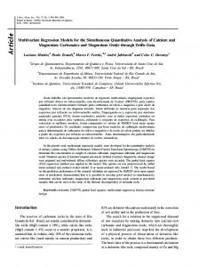
Journal of Business & Economics Research – August 2007

Volume 5, Number 8

Isolating The Key Variables For Regression Models In Enterprise Software Acquisition Decisions: A Blocking Technique Rolando Pena-Sanchez, (Email: [email protected]), Texas A&M International University Jacques Verville, (Email: [email protected]), Texas A&M International University Christine Bernadas, (Email: [email protected]), Texas A&M International University

ABSTRACT Often researchers in the field of information systems face problems related to the variable selection for model building; as well as difficulties associated to their data (small sample and/or non normality). The goal of this article is to present an original statistical blocking-technique based on relative variability for screening of variables in multivariate regression models. We applied the blocking-technique and a nonparametric bootstrapping method to the data collected on the USASouth border for a research concerning enterprise software (ES) acquisition contracts. Three mutually exclusive blocks of relative variability for the response variables were formed and their corresponding regression models were built and explained. A conclusion was drawn about the decreasing tendency on the adjusted coefficient of determination (R 2adj) magnitudes when the blocks change from low (L) to high (H) condition of relative variability. The obtained models (via stepwise regression) exhibited significant p-values (0.0001).

1. INTRODUCTION

I

n this research we present an original statistical blocking-technique based on relative variability to support the screening of variables for multivariate regression models. We applied such blocking-procedure and a nonparametric bootstrapping method (Pena-Sanchez, 2005a) to analyze the data collected from the USASouth border for a research concerning enterprise software (ES) acquisition contracts. Researchers are often faced with small samples where data does not meet the requirements for conventional (parametric) statistical methods. The reason could be due to conceptual problems (Pullman and Eaton, 2001), low turn out rate from participants in laboratory experiments, or low responses from mail surveys and/or other issues related to the difficulty of collecting data (Leedy and Ormrod, 2001). In the past decade or so, bootstrapping has proven to be a popular method for small sample size data sets. It has been widely used in such fields as astronomy, biology, economics, engineering, finance, medicine, molecular biology and genetics; however, it has not been widely used within the field of information systems or business management as a whole. What is bootstrapping? Bootstrapping is the concept of re-sampling data randomly multiple times and drawing statistical conclusions from the data set. Bootstrapping was instigated by Efron (1979). It can be used in a wide variety of scenarios. For example; bootstrapping can correctly estimate the variance of sample median; it also can estimate the error rates in a linear discrimination problem, out performing “cross-validation,” another nonparametric estimation method (Efron, 1979). The bootstrapping method is susceptible to help researchers to overcome some of their data problems and find interesting results when other traditional techniques can‟t be used.

57

Journal of Business & Economics Research – August 2007

Volume 5, Number 8

2. DATA AND METHODOLOGY 2.1 Data The research used as example was carried out with a random sample of 52 (multivariate) observations from the USA-South border around Laredo, Texas (Web County) during summer 2004. The data was collected via a mail survey sent to IT executives in charge of ES contracting; the survey questionnaire (Appendix B) was developed based on a previous research project on ES acquisition practices (Verville, 2000). A small pilot study, conducted with 30 respondents, was used to pre-test the instrument and to identify any ambiguities and other problems with the survey questionnaire. The survey had 36 questions (named X1 to X36) and to answer the respondents use a Likert response scale from 1 to 7 from “not very important” (1) to “very important” (7). The descriptive labels for each of the 36 variables are shown in the Appendix A. 2.2 Methodology We divided the methodology in three phases: 1) 2) 3)

Hypothesis Testing, described in Section 2.2.1, tests the differences among central location parameters for all response-variables via nonparametric procedures (see Table 3). Bootstrapping Method, described in Section 2.2.2, is technique for estimating the relative variability (coefficient of variation) for all response-variables X1 to X36 (see Table 6). A Blocking Technique, described in Section 2.2.3, is a procedure for conforming the "blocks of relative variability": low, moderated, and high (see Table 7). Thus, inside each block, the last step is to estimate the most significant models (Mood et al, 1974) of multiple linear regression via stepwise regression (see Table 8).

2.2.1 Nonparametric Hypotheses Testing 2.2.1.1. The Kruskal-Wallis test This test is used under the assumption of independence between k samples (k≥ 3). The involved hypotheses for the Kruskal-Wallis test are: Ho: All the k population distribution functions are equal. Ha: At least one the populations tend to yield larger observations than at least on the others populations. Due to the sensitivity of this test about the differences between central location parameters in the populations, the alternative hypothesis may be stated as: Ha: The k populations do not all have equal central location parameters. 2.2.1.2. The Friedman Test Under the Kruskal-Wallis test it is assumed that each “Executive” has been rating each variable (from X 1 to X36) in an independent way for each criterion: levels of X 38 (see Table 4) and/or X45 (see Table 5); but taking in consideration the fact that the data are composed by related samples (Pohlen and Coleman 2005), given that for each criterion, the 36 ratings (one rating for each variable) belong to the same “Executive”; thus, there is a link among the 36 responses: “Executive”; then, independence is no longer valid. Therefore the appropriated statistical contrast for this case is the Friedman test, using “Executive” as a blocking factor. The involved hypotheses in the case of the Friedman test, (given b blocks (Executives) and k treatments (X 38 and/or X45)) also called “control factors” (Pena-Sanchez, 2005b) are: 58

Journal of Business & Economics Research – August 2007

Volume 5, Number 8

Ho: Each ranking of the random variables within a block is equally probable; which is equivalent to say: The location parameters i are equal within each block j; where i=1,2, …, k; j=1,2, …, b Ha: At least one of the groups of classification (treatments: levels of X 38 and/or X45) tended to yield larger observations than at least one of the other groups of classification; which is equivalent to say that at least one of the location parameters i is not equal to the others within at least one block. 2.2.2. Bootstrapping Method This is a resampling technique, in which the original data are repeatedly sampled with replacement to generate a large bootstrap sample for model estimation (see Table 1). Thus, the confidence interval estimates for the parameters are no longer evaluated under statistical assumptions, but instead are calculated using the bootstrapped (empirical) observations.

Table 1 Steps of the bootstrapping technique Step 1. Read observations {x1, x2, …, xn} Data

Action Imports the n observations and save these as the „Data‟ vector.

2. Repeat m, m ≥ 100 3. Sample n Data: Output

Repeat the next steps m times. To sample n observations with replacement. The output represents the bootstrap sample. Find the mean of the vector Output and save its value as Value1 To keep track of the result of each simulation, this is attached into the Total vector. Ends a loop, and send the process back to a „Repeat‟ statement. To evaluate the mean of all Value1, and save this as M, which is the bootstrapped mean (point) estimate for  Find 2.5th and 97.5th percentiles, and save these as P L and PU, which represents the lower and upper limits of a bootstrapped 95% confidence interval estimate for  Exports the results.

4. Mean of Output: Value1 5. Track Value1: Total 6. End 7. Global mean of Value1: M 8. Total: Percent (PL =2.5, PU =97.5)

9. Write: Output, Value1, M, P L and PU

2.2.3. A Blocking Technique Three blocks of relative variability: low, moderated, and high; have been conformed (see Table 7). The conformation criterion is based on the relative variability of the data (X1 to X36) through its coefficient of variation: CV(Xi)%=(Standard deviation of Xi / Mean of Xi)100%. Criteria: Block L: Low (CV%< Q1), Block M: Moderated (Q1≤ CV%≤ Q3), and Block H: High (CV%>Q 3 ). Where Q1 and Q3 represent the first (25%) and the third quartile (75%) respectively. Q 1 is also named as the twenty-five percentile, similarly Q3 represents the seventy-five percentile; all of this with respect to the total distribution of CV%. Thus, Block L contains a set of response variables with high stability and/or low (L) relative variability; while Block H contains a set of response variables with low stability and/or high (H) relative variability. The group of variables with a condition of moderated stability and/or a moderated (M) relative variability is contained in Block M. This notion of "stability" is based upon the ordered measures (quartiles) of the coefficient of variation (CV%). As we can perceive, the response variables have been grouped in mutually exclusive blocks of relative variability.

59

Journal of Business & Economics Research – August 2007

Volume 5, Number 8

After this conformation of blocks, the last step is to estimate (for each block) the most significant models (Mood et al, 1974) of multiple regressions via stepwise regression (see Table 8). 3. RESULTS Given the limited number of observations (n=52), the fact that many variables do not meet parametric F-test assumptions like normality (Kolmogorov-Smirnov test), and the recognition that some of them do not meet homocedasticity (Levene test) of the variances (see Table 2), then the use of a nonparametric statistical method based on ranks (Conover, 1999), such as the Friedman test described in the Section 2.2.1.2 is justified.

Table 2 Kolmogorov-Smirnov test for normality, and Levene test for homogeneity of variances (homocedasticity) Variables Test and p-values Decision X1 to X6, X8 to X13, Kolmogorov-Smirnov Reject Normality X15, X17 to X32, p-values < 0.05 X34 to X36 X7, X21, X27, X28, X31 Levene p-values < 0.05 Reject Homocedasticity

Variables X1 to X36

Table 3 Friedman test for the equality of location parameters Friedman’s test p-value > 0.05

Decision Do not Reject Ho

Table 4 Frequency distribution for X38: What is your job title/area of responsibility? X38 What is your job title/area of responsibility? Frequency Percent IT Management 2 3.8 Purchasing 6 11.5 Legal 3 5.8 User 12 23.1 Other 29 55.8 Total 52 100.0

Table 5 Frequency distribution for X45: What is your Job/area of responsibility?, where the first 3 categories in Table 4 have been grouped in one category (see Section 2.2.1.2). X45: What is your Job/area of Frequency Percent responsibility? CIO, IT Management, Purchasing, 11 21.2 and/or Legal User 12 23.1 Other: Advisor, Consultant, and/or External Contractor 29 55.8 Total 52 100.0

Table 2 justifies the use of nonparametric statistics (p-values0.05) among the 3 types of Job/area of responsibility defined by the variable X45 in Table 5. We got the same conclusion (pvalues>0.05) among the 5 types of Job-title/area of responsibility defined by the variable X38 in Table 4. Thus, Tables 4 and 5 contain the treatments (categories) required in the Friedman test; the other elements or components in this test 60

Journal of Business & Economics Research – August 2007

Volume 5, Number 8

are: data (response variables X1 to x36) and the blocking factor: Executives. Unfortunately we don‟t have sufficient sampling evidence or more information to reject the null hypothesis (H o) presented in the section 2.2.1.2. Knowing that the sample size was relatively small to go forward with the confidence interval estimates (Morrison, 2005), we decided to use the bootstrapping technique described in Table 1, to generate a large sample from the original distribution of the 52 multivariate observations; the results are shown in Table 6.

Table 6 Bootstrapped estimates according to the syntax described in Table 1. Notation: XC: Variablecondition, X : mean, S: Std. Deviation, CV%: Coefficient of Variation in percent, L95: Lower limit, and U95: Upper limit of the 95% Confidence Interval for the CV% X S CV% L95 U95 X S CV% L95 U95

X

X1M X2H X3M X4M X5M X6M X7M X8M X9H X10H X11M X12M X13 L X14H X15H X16M X17H X18M

5.74 5.39 5.89 5.65 5.54 5.64 5.56 5.45 5.54 5.18 5.96 5.58 5.94 4.94 5.16 5.35 5.32 6.02

X

1.19 1.40 1.17 1.23 1.26 1.17 1.23 1.25 1.53 1.74 1.18 1.30 1.02 1.55 1.54 1.30 1.37 1.17

20.76 25.94 19.79 21.78 22.67 20.71 22.04 23.02 27.56 33.54 19.78 23.30 17.22 31.29 29.85 24.26 25.83 19.52

17.40 20.74 16.99 16.45 18.83 16.47 17.98 18.09 22.01 27.51 15.01 17.82 12.21 25.93 23.43 20.02 19.98 14.80

24.13 31.38 22.70 27.16 26.72 25.77 26.23 28.27 33.08 40.21 25.54 29.03 23.26 36.69 36.87 29.30 32.26 25.13

X19H X20M X21H X22H X23L X24L X25M X26M X27M X28L X29L X30L X31L X32L X33M X34M X35M X36L

5.58 5.31 5.75 5.56 5.75 5.97 5.75 5.37 5.44 5.62 5.98 5.94 5.99 6.15 5.33 5.73 5.75 6.17

1.41 1.33 1.46 1.42 1.06 1.03 1.26 1.27 1.24 1.02 1.08 0.946 0.940 0.791 1.31 1.07 1.36 0.973

25.21 25.04 25.44 25.56 18.47 17.29 21.85 23.62 22.76 18.13 18.06 15.94 15.68 12.84 24.61 18.71 23.71 15.76

20.19 20.18 19.75 20.87 15.16 14.04 17.05 20.63 17.84 15.68 13.87 13.35 13.03 11.14 20.70 15.01 18.77 13.09

30.92 30.10 31.18 29.92 22.28 20.34 27.15 26.81 28.47 20.40 22.44 18.65 18.66 14.48 28.48 23.02 29.18 18.64

Thus, the set of 36 response-variables can be grouped in 3 mutually exclusive subsets of bootstrapped relative variability (condition): L: low (CV%< Q1), M: moderated (Q1≤ CV%≤ Q3), and H: high (CV%>Q 3 ). Where the first quartile is Q1=18.53, and the third quartile is Q3=25.17. The blocks with the variables grouped under this criterion are shown in (Table 7), while the blocks with the variables‟ labels appear in Appendix A.

Table 7 Blocks of response variables in terms of stability and/or relative variability Block L Block M Block H Response variables with high stability Response variables with moderated Response variables with low stability and/or low (L) relative variability stability and/or moderated (M) and/or high (H) relative variability (CV%Q 3 ) (Q1≤ CV%≤ Q3) X13, X23, X24, X28, X29, X30, X31, X1, X3, X4, X5, X6, X7, X8, X11, X12, X2, X9, X10, X14, X15, X17, X19, X32, X36 X16, X18, X20, X25, X26, X27, X33, X21, X22 X34, X35‟

61

Journal of Business & Economics Research – August 2007

Volume 5, Number 8

The first block (L) contains variables where the respondents show a consensus among their opinions about the importance of these variables in ES acquisition contracts; while the block M contains variables related to contingencies and contractual assurances. The block H contains variables where the respondents manifest the fewest consensuses. By rotating all variables positions into each block and into each model via stepwise regression, Table 8 shows the best combination of independent variables: highest value of the adjusted coefficient of determination (R2adj) for each block (see Table 8).

Block

Dependent variable

L

X23

M

X26

H

X17

Table 8 Multiple regression models estimates per block of relative variability Estimates of the Estimates of unstandardized the standardized F coefficients x for coefficients ‟x for R2adj statistic the independent the independent Variables (x) variables (x) 0L = -1.754 24 = 0.283 ‟24 = 0.274 13 = 0.455 ‟13 =0.444 0.669 26.801 30= 0.263 ‟30 = 0.233 32 = 0.251 ‟32 = 0.186 0M = 0.554 25 = 0.596 ‟25 = 0.595 7 = 0.364 ‟7 = 0.352, 0.632 22.884 20 = -0.311 ‟20 = -0.327 35 = 0.177 ‟35 = 0.190 0H = 0.141 15 = 0.428 ‟15 = 0.476 22 = 0.276 ‟22 = 0.283 0.554 22.147 21 = 0.250 ‟21 = 0.265

p-value

0.0001

0.0001

0.0001

We obtain in each block via stepwise regression a model (Figures 1 to 3), which maximize the significance of the data inside the blocks (significant p-values at 0.0001).

Figure 1 Model for block L (block of low relative variability). X13: Transfer the software Width indicate strength of the link

X24: Forward compatibility when operating systems (OS) changes

+ +

X30: Indemnity by vendor for infringement

X32: Cap on future prices

X23: Clear differences between software support and a new license

+ +

The four variables X13, X24, X30 and X32 contribute to the clarification between software support and new license (positive sign of the relationships).

62

Journal of Business & Economics Research – August 2007

Volume 5, Number 8

From their perspective, what is associated to normal changes (e.g. transfers or operating systems changes) should entail few or no costs for their company. Based on this view, the acquisition contract should clearly reflect this position and protect them to this effect. This contract should also prevent excessive increase in prices in case of new licenses. This point of view can be explained in part by the fact that USA-South border companies are medium and small enterprises. The acquisition of the ES has already put a strain on their budget; they want to insure that the rest of the ES life is as costless as possible.

Figure 2 Model for block M (block of moderated relative variability). X25: Compatibility if hardware changes

Width indicate strength of the link

+

X07: Written notice for acceptance

+ X26: Compatibility of ES with other software of the same vendor

−

X20: Remedies for vendor‟s nonperformance

+ X35: Escrow agreements

In this block, the independent variables are mainly oriented to the contingencies in the eventuality of relationships going wrong. During the ES acquisition and particularly for USA-South border and Mexican companies, a strong relationship with a vendor is created (Verville et al., 2004). If a company is acquiring an ES from a specific vendor, there is a very high probability that they will continue to do business with this vendor (i.e. buy other software if they are available, no best-breed acquisition). Compatibility, written notice, remedies, and agreements are ways to formalize the link buyer-vendor, because the compatibility between products is a way to reinforce this link.

Figure 3 Model for block H (block of high relative variability). X15: Limited liability Width indicate strength of the link

X22: Incentives to licensors‟ performance

+ +

X21: Remedies for consequential damages

X17: The use of your own forms

+

According to this model, the company, which will acquire an ES, should protect itself, and insure via the contract that it keeps the control.

63

Journal of Business & Economics Research – August 2007

Volume 5, Number 8

4. CONCLUSIONS In this article, we have presented an original statistical blocking-technique based on the relative variability for screening of variables in multivariate regression models. We applied the blocking-technique and a nonparametric bootstrapping method to the data collected on the USA-South border for a research concerning enterprise software (ES) acquisition contracts. Before applying this method, the data collected were unusable through traditional statistical methods (due to small samples and non-normal data). Afterward, three mutually exclusive blocks of relative variability for the response variables were formed, and their regression models were built (Nishii, 1984) and explained. Thus, when the classical statistical methods are restricted by the size and type of data, the researchers can now follow new research avenues to confirm the results obtained. For example, from Table 8, we have drawn a conclusion about the decreasing tendency on the R2adj magnitudes when the blocks change from low (L) to high (H) condition of relative variability. Then, a relevant result under this blocking technique was obtained: the three estimated models (through stepwise regression) exhibited significant p-values (0.0001). Our conclusion from Figure 1, is that reviewing the block of independent variables (X13, X24, X30, and X32), the respondents in the USA-South border tend to associate strongly the responsibilities of the vendors linked with costs of changes or problems with a will to clearly specify what is supported (e.g. included in a maintenance/support contract) and what should be re-negotiated as a new license (X23). From Figure 2, we conclude that the block of independent variables (X25, X07, and X35) tend to contribute to the contractual assurances regarding forward compatibility of the software with changes in other software from same vendor with the exception of “Remedies for vendor's non-performance” (X20), which presents a negative relationship with “The compatibility of ES with other software of the same vendor” (X26). Thus, for the respondents, the increase of remedies decreases their assurance regarding forward compatibility of the software with this other software of the same vendor. The sign can be explained by the fact that the formalization of the remedies in the contract is making the formalization of the compatibility with the vendor‟s software less important. This relationship and its sign will require further research (e.g. how can the sign be better explained? Is-it a specificity of USA-South border companies or with a USA wide or Mexican wide data with found the same relationship and sign?). While the Figure 3 shows that the block of independent variables (X15, X22, and X21) re-enforce the will of the buyers to keep/use their own forms in place of the licensing contract (X17). Clearly, this model is more related to control.

64

Journal of Business & Economics Research – August 2007

Volume 5, Number 8

Appendix A Blocks of response-variables in terms of stability and/or relative variability condition Block L Block M Block H Response variables with high stability Response variables with moderated Response variables with low stability and/or low (L) relative variability stability and/or moderated (M) and/or high (H) relative variability (CV%< Q1) relative variability (CV%>Q 3 ) (Q1≤ CV%≤ Q3) X13 In situations other than enterprisewide licenses, the right to transfer the software to other equipment and operating systems at no costs X23 Contractually defined difference(s) between (1) enhancements, releases, versions, etc., that you receive by subscribing to software support, and (2) those the vendor insists are a new product requiring a new license X24 Contractual assurances regarding forward compatibility of the software with changes in operating systems (OS) X28 Contingencies for what would occur regarding support, upgrades, etc., should the organization acquire another company or divest a division, or if the vendor goes bankrupt, other similar situations arise X29 Vendor‟s responsibility to meet the cost of procuring alternative third-party support if the vendor fails to provide adequate and timely service X30 The vendor accepts to indemnify the organization for all losses, damages or liabilities arising from the infringement or alleged infringement of such patents, trademarks, trade secrets, copyrights or any other pertaining to intellectual property rights X31 The vendor warrants that the services provided to the organization shall not infringe upon any patent, trademark, trade secret, copyright, or any other right relating to intellectual property: rights in force, recorded, or recognized X32 A cap on future maintenance prices X36 Warranties and liabilities

X1 The right to assign the software license to a new corporate entity resulting from a merger, consolidation, acquisition or divestiture X3 The right to assign the software license to or allow the software to be used by an outside entity if you outsource your data processing operations X4 The right to re-assign software licenses within the corporate entity X5 The right to develop and own derivative works (i.e., code changes, translation, adaptations, customizations) based upon the software X6 The right to customize during the software acceptance period X7 The right to define software acceptance as occurring only upon your written notice X8 The right to establish acceptance procedure X11 The right to terminate for convenience X12 The right to port the software to any platform supported by the vendor at no or minimum charge X16 Prohibition against devices in the software that control your compliance with the software license X18 Licenses that permit unlimited use within your corporate or Organization X20 Specific remedies for vendor‟s nonperformance X25 Contractual assurances regarding forward compatibility of the software with changes in hardware X26 Contractual assurances regarding forward compatibility of the software with changes in other software from the same vendor X27 Permission to exempt individual employees/ contractors from signing documents that acknowledge confidentiality of software or to bind them to terms of the license X33 Avoidance of partial payments to vendors based on checkpoints X34 Insurance: the vendor agrees to acquire and keep in force at its expense insurance, comprehensive general liability insurance, and workers compensation insurance, and to provide evidence of such insurance X35 Escrow agreements (i.e., source or object code access, etc.)

65

X2 The right to use the software for the benefit of a business unit formerly within your corporate organization which has been sold X9 The right to own the source code (source code ownership) X10 The right to terminate for convenience X14 In situations other than enterprisewide licenses, the right to use the software for the benefit of other entities X15 Limited liability for breach of your obligations under the software license agreement X17 Use of your own form in place of the licenser‟s form for licensing contracts X19 License for any third-party software application used under this contract: the vendor guarantees that the organization May use such software application without infringing upon any third-party intellectual property rights X21 A remedy for consequential damages that you suffer X22 Incentives to licensors to reward their performance in providing services

Journal of Business & Economics Research – August 2007

Volume 5, Number 8

REFERENCES 1. 2. 3. 4. 5. 6. 7.

8. 9. 10. 11. 12. 13. 14.

Conover, W. J. (1999). Practical Nonparametric Statistics, 3rd. Edition John Wiley & Sons. Efron, B. (1979).Bootstrap Methods: Another Look at the Jackknife. The Annals of Statistics, 7, 1-26. Leedy, P. D., and Ormrod, J. E. (2001). Practical Research: Planning and Design. Merryll Prentice Hall. Seventh Edition. Mood, A. M., Graybill, F.A. and Boes, D. C. (1974). Introduction to the theory of statistics. McGraw-Hill. Third Edition. Morrison, D. F. (2005). Multivariate Statistical Methods. 4th Edition. Thomson Learning, Inc. Nishii, R. (1984) Asymptotic properties of criteria for selection of variables in multiple regression. The Annals of Statistics. Vol. 12, No. 2. 758-765. Pena-Sanchez, R. (2005a) A Nonparametric Comparison of the Per Capita Yearly Economic Needs for the Water Supply in the USA-Mexico Border Region. International Business and Economics Research Journal. 4(6), 35-46. Pena-Sanchez, R. (2005b) A Case of Test-Results in RFID: A Technology to Improve Competitiveness in Logistics. American Society for Competitiveness. Competition Forum Vol. 3. pp. 98-107. Pohlen, T. R. and Coleman, B. J. (2005). Evaluating Internal Operations and Supply Chain Performance Using EVA and ABC. Advanced Management Journal, 70(2), 45-59. Pullman, M. E. and Eaton, F. F. (2001). Optimizing service attributes: The seller‟s utility problem. The Journal of the Decision Sciences Institute. 32(2), 251-275. Verville, J. C. (2000) An empirical study of organizational buying behavior: a critical investigation of the acquisition of ERP software. Dissertation, Universite Laval, Quebec. Verville, J. (2000) A Model of ERP Acquisition Process, Proceedings of the 31st Annual Conference of Decision Science Institute, November 2000. Verville, J. (2000) The Acquisition Process for ERP Software: The Case of International Air. Proceedings of the 1st Global Information Technology Management (GITM) World Conference, June 2000. Verville J., Flores O., and Bernadas C. (2004) Critical Factors Affecting the Selection Process of Enterprise Software: A Study of IS Managers Perceptions in the Mexican Service and Manufacturing Industries‟, Proceedings of the 21st Annual Association of Management (AoM) Conference, Vol. 21, No. 2, pp 255-56.

66