Jackpine: A Benchmark to Evaluate Spatial Database Performance

Jackpine: A Benchmark to Evaluate Spatial Database Performance Suprio Ray, Bogdan Simion, Angela Demke Brown Department of Computer Science, University of Toronto Toronto, Ontario, Canada {suprio, bogdan, demke}@cs.toronto.edu

Abstract— The volume of spatial data generated and consumed is rising exponentially and new applications are emerging as the costs of storage, processing power and network bandwidth continue to decline. Database support for spatial operations is fast becoming a necessity rather than a niche feature provided by a few products. However, the spatial functionality offered by current commercial and open-source relational databases differs significantly in terms of available features, true geodetic support, spatial functions and indexing. Benchmarks play a crucial role in evaluating the functionality and performance of a particular database, both for application users and developers, and for the database developers themselves. In contrast to transaction processing, however, there is no standard, widely used benchmark for spatial database operations. In this paper, we present a spatial database benchmark called Jackpine. Our benchmark is portable (it can support any database with a JDBC driver implementation) and includes both micro benchmarks and macro workload scenarios. The micro benchmark component tests basic spatial operations in isolation; it consists of queries based on the Dimensionally Extended 9intersection model of topological relations and queries based on spatial analysis functions. Each macro workload includes a series of queries that are based on a common spatial data application. These macro scenarios include map search and browsing, geocoding, reverse geocoding, flood risk analysis, land information management and toxic spill analysis. We use Jackpine to evaluate the spatial features in 2 open source databases and 1 commercial offering.

I. I NTRODUCTION Spatial data is everywhere. Geospatial Web services such as Google Maps, in-vehicle GPS navigation systems, GPSenabled mobile phones, and a host of accompanying locationbased services have become part of our daily experience. Enormous quantities of spatial data is constantly being generated from various sources such as satellites, sensors and mobile devices. NASA’s Earth Observing System (EOS), for instance, generates 1 terabyte of data every day [1]. A decade ago, it was estimated that 80% of all business data stored in existing databases had spatial attributes [2]. The percentage today is probably even higher, as the ability to track customers and inventory has become cheaper and easier. The deluge of spatial data and increasingly sophisticated end-user demand is changing the landscape for Geographic Information Systems (GIS). A GIS is concerned with organizing spatial data into real-world geographical features such as landmarks, roads and rivers. Spatial queries then can be used to extract useful information related to features of interest

with any location criteria. The term “spatial database” refers to relational database management systems that support spatial data types in the same way as any other data in the database. Although spatial support was once a niche feature provided by high-end systems for a small set of customers, or found only in research systems, it is now widely used with new applications appearing regularly. The degree to which spatial functions are supported in traditional relational database systems (RDBMS) varies widely. For example, true geodetic support (i.e., support for true measurement along a spherical coordinate) is offered in Oracle, DB2 and SQL Server, but not by MySQL, or Ingres. PostgreSQL has true geodetic support only for point-to-point non-indexed distance functions. Informix provides both a no-cost Spatial module (which lacks geodetic support) and a Geodetic module (which is not free). In terms of spatial functions, SQL Server, Oracle, DB2, Informix and PostgreSQL support spatial predicate functions defined by the Open Geospatial Consortium (OGC) [3], as well as custom geodetic functions. MySQL only supports OGC functions using minimum bounding rectangles (MBRs). Support for spatial indexing also varies, with most of the spatially enabled databases offering the R-tree index [4], except for SQL Server which provides a Grid. PostgreSQL supports a generalized R-tree index called GiST [5]. Finally, the cost of these different options also varies widely. The diversity of offerings in this rapidly growing domain naturally gives rise to performance questions from multiple stakeholders. Developers or organizations deploying spatially enabled applications want to evaluate which spatial database will support their needs in the most cost-effective manner. Database researchers and developers want to know which features or operations limit performance in real use, to focus the design and implementation of new algorithms. Finally, systems researchers and architects want to understand the stresses imposed on processor, memory, and storage resources by spatial database workloads. These types of questions are the purview of benchmarking. Unfortunately, there is no widely used, industry standard spatial benchmark. The Transaction Processing Performance Council (TPC) [6], which is devoted to defining transaction processing and database benchmarks for diverse workloads, has not yet addressed spatial workloads. Although a number of research papers have proposed spatial benchmarks, these are typically limited in scope and/or are designed to test a specific

c 2011 IEEE. This is the authors’ version of the work. Not for redistribution. Published in ICDE

feature or application. None of these have gained widespread acceptance or adoption. Jackpine is a spatial database benchmark intended to fill this gap. Sim et al., in a study on the value of benchmarking, noted that the adoption of a benchmark fosters both community building and technical advances in a research area [7]. Our aim is to provide the basis of such a benchmark, providing both micro benchmark coverage of basic spatial operations as well as modeling a number of real-world applications for spatial databases. As systems researchers, we stand as outsiders to the database and GIS communities. Our ultimate aim is to see how low-level systems software is exercised by spatial database workloads. We believe this affords some advantages in the design of a benchmark, as we have no bias toward (or against) any particular implementation or application. On the other hand, the application scenarios we have modeled are not as realistic as they could be since we may lack detailed knowledge of how these systems are used in practice. Our hope is that Jackpine will provide the basis for ongoing discussion and refinement within the community, leading to a benchmark that will be widely used. The rest of this paper is organized as follows. We review related work in Section II. In Section III we describe the micro and macro query scenarios included in Jackpine, the datasets used, and the implementation details. Sections IV and V present the experimental setup and the results from a comparative study of three databases with Jackpine. We end with a discussion of the strengths and limitations of this benchmark in Section VI. II. R ELATED W ORK The objective of benchmarking is to evaluate a system against a reference system in order to compare performance based on various criteria. Database benchmarks can be used to compare different hardware configurations, different database vendor software and different software releases. They play a key role in supporting business decisions on what database to use, as well as database research and development. In this section we review general database benchmarks as well as spatial database benchmarks. A. Non-spatial database benchmarks There are many commercial and free database benchmarks. They differ in their approaches to quantify system performance, workloads and features; we focus here on the most well-known ones. Although the goal of the database benchmarks is to simulate real-world workloads as closely as possible, they may not reflect an organization’s actual workload. For this reason, many of the benchmarks choose a few specific business process scenarios and evaluate the databases against synthetic workloads. The TPC benchmarks [6] and DBT [8] are prime instances of this. Others use variations of generic database operations - select, project, join and update to generate the workloads. The Wisconsin Benchmark [9] and Bristlecone [10] are in this category.

The Wisconsin Benchmark is one of the first attempts to develop a scientific methodology for performance evaluation of databases. The benchmark consists of a standard set of queries which measure the cost of different relational operations. Bristlecone is a recent database performance testing utility that is similar in spirit to the Wisconsin Benchmark. Bristlecone provides the ability to create flexible test scenarios by varying the database operations, number of threads, number of tables, number of rows per table etc. Since it is implemented in Java, Bristlecone offers the possibility to support many different databases that have a JDBC driver implementation available. Although it is designed to evaluate database clusters, Bristlecone can also be used on single database instances. Because of its flexibility, we have used Bristlecone as the basis for Jackpine. The Transaction Processing Performance Council (TPC) is a non-profit organization devoted to defining database related benchmarks. TPC has developed several benchmarks, each suited to a different workload domain, which are generally considered the industry standard by many enterprises. For example, TPC-C is an On-line Transaction Processing (OLTP) benchmark that simulates an order-entry environment. The transactions involved in this benchmark include entering and delivering orders, recording payments, checking the status of the orders, and monitoring the level of stocks at the warehouse. TPC-E is another benchmark that models the OLTP workload after a brokerage firm. TPC-H is a decision support benchmark that is characterized by the execution of queries with high degree of complexity and concurrent data modifications. Notably, the TPC reports price/performance metrics, highlighting the cost of achieving a particular performance level. None of the existing TPC benchmarks address spatial database workloads. The popularity of the TPC benchmarks has spawned a number of open source clones. The Open Source Development Labs Database Test Suite [8], known as DBT, is modeled after the TPC benchmarks, but differs in a few areas and is not certified. DBT is among the most comprehensive of all open source benchmark suites. jTPCC [11] and BenchmarkSQL [12] are open source Java implementations that resemble TPC-C. However, they are not fully compliant. TPCC-UVa [13] is an open source implementation that includes the functionalities specified by TPC-C. However, the focus of TPCC-UVa is to compare the performance of different Linux file systems. It also attempts to evaluate relative system performance in multicore CPU systems as opposed to a single core system. In addition, there are several open source benchmarks that are not modeled after the TPC. PolePosition [14] is a benchmark suite that was developed to compare database engines and object-relational mapping technology. OSDB [15] is an open source database test suite that is based on the ANSI SQL Scalable and Portable Benchmark (AS3AP), as documented by Grey [16]. SPECweb2009 [17] is a benchmark to evaluate the performance of web servers when serving both static and dynamic pages. The benchmark itself does not include or specify any of the web server software. However, a common web

c 2011 IEEE. This is the authors’ version of the work. Not for redistribution. Published in ICDE

server archicture uses a multi-tier environment with a backend database server. Thus, although SPECweb2009 is not a database benchmark, it provides indirect evidence of the underlying database performance. There are several other benchmarking tools available but they are not as commonly used. None of the database benchmarks discussed so far assess the performance of spatial features. B. Spatial Database Benchmarks Objects in a geographic information system (GIS) are stored in a two-dimensional space and the queries asked of such a system are different from regular SQL queries. Typical geospatial queries [18] include partial matching queries, range queries, nearest-neighbor queries and where-am-I queries. However, as an emerging application domain, novel business scenarios and bleeding edge Web applications are being developed with GIS. Moreover, spatial data features arise in non-geographic applications as well, although GIS is still the largest application area. As a result, one of the key challenges in the development of a spatial benchmark is defining the workloads. Moreover, many spatial functions provided by different relational database vendors are still work-in-progress and the available features across different databases are not always standard offerings. Thanks to the work of the Open Geospatial Consortium (OGC) [3], however, standards for spatial functions have been defined and are being adopted by many databases. These developments make this a promising time to revisit the design of a spatial benchamrk. There have been only a handful of research projects that attempted to benchmark spatial database systems. The best known existing benchmark for spatial databases is SEQUOIA 2000 [19], which was specifically designed to be an earth sciences benchmark and focused on raster data. In contrast, many of today’s emerging GIS applications, and the spatial database extensions, operate on vector data. In addition, while the queries specified by SEQUOIA 2000 are all relevant to Earth Sciences, they are all isolated queries rather than a sample Earth Sciences workload. Also, there is no indication that they represent a complete set of queries that would be used in this domain. Finally, SEQUOIA 2000 specifies only the queries, and rules for reporting price/performance. It includes no implementation and no test or timing harness, making it difficult for others to adopt. VESPA [20] is a vector based spatial database benchmark that includes a range of query and update tasks that could be executed over synthetic data sets. It was used to compare PostgreSQL with the Rock & Roll deductive object oriented database [21]. VESPA includes a large number of “tasks” (essentially, individual queries) that test update, set union, containment, overlap, intersect, adjacent, search inside, measurement, and analysis operations. Although there are a large number of operations, it is difficult to assess how comprehensively these operations cover the available spatial functions. The use of synthetic data solves problems with scaling, but raises issues of how well it represents real-world

data, which can have an impact on measured performance. Finally, VESPA does not include any attempt to model real spatial workloads and is not publicly available. In recent years there have been very few reports of spatial benchmarking efforts. The few that exist were conducted on an ad hoc basis, simply by executing a few spatial queries against one or two databases and comparing the latency and throughput. Power [22] compared MySQL and PostgreSQL/PostGIS using a small dataset and contrived queries. The author suggested that the study used a dataset that is almost trivial and used rather simple spatial queries. Dynamark [23] and BASIS [24] are benchmarks that are geared towards evaluating spatial index structures, rather than full database systems. In the following section we describe the design of Jackpine, the benchmark we have developed for vector spatial databases. We include both micro benchmark operations, to assess the performance of individual spatial functions, and macro workload scenarios to assess the expected performance with real workloads. III. T HE B ENCHMARK One of our goals in developing Jackpine is to be able to support as many different databases as possible, with minimal effort. We believe this is a key feature if the benchmark is to achieve widespread adoption by other users. Another objective of Jackpine is to include a comprehensive set of workloads, that would include basic spatial operations on one hand, and representative real-world applications on the other. To this end, Jackpine consists of two different parts: a micro benchmark and a macro benchmark. The micro benchmark is comprised of a number of spatial join queries with topological relationships, several queries with spatial analysis functions, and data loading queries. The macro benchmark includes queries that are modeled on 6 different real-world spatial applications. A. Implementation Overview To leverage the development effort of existing database benchmarks, we evaluated a number of open source options. Our motivation was to reuse the test harness or part of the implementation of the chosen benchmark. In our evaluation, Bristlecone [10] fared better than the others, in terms of support for open-source databases, available features and extensibility. Bristlecone allows running test cases with systematically varying parameters. Also, Bristlecone is written in Java, allowing it to be used with any database that provides a JDBC driver implementation. We thus chose to use the test harness of Bristlecone as the basis of our own implementation.1 A key concept in our benchmark is the spatial scenario, which is an extension of a scenario in Bristlecone. A spatial scenario is essentially a test case that includes SQL queries and the specification of various parameters. A Java class implements the functionalities relevant to a particular spatial scenario. The run-time parameters such as the number of 1 This

is reflected in the name Jackpine.

c 2011 IEEE. This is the authors’ version of the work. Not for redistribution. Published in ICDE

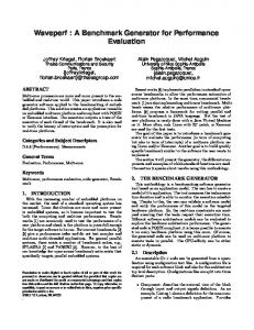
Fig. 1.

Benchmark output report

TABLE I DATABASE TABLES USED FOR MICRO AND MACRO BENCHMARK Database table

Geometry

edges merge

line

pointlm merge arealm merge areawater merge gnis names09 s fld haz ar s gen struct land use 2006 parcels2008 hospitals s wtr ar frontyard parking restrictions landfills geocoder address cityinfo

point polygon polygon point polygon line polygon polygon point polygon polygon point point

Cardinality 5895060

Data file size (KB) 1651629

Index file size (KB) 416972

13441 5963 374053 103413 3403 938 404599 321578 48 3 76 79 2587672 41660

920 28490 200734 10225 70339 93 162400 131808 7 2813 321 30 214835 5836

985 1644 26144 10562 267 71 36327 25179 5 4 7 9 8653 2974

warmup runs, number of iterations, number of threads, width and length of data selected, databases to run against, etc. are specified in a properties file. Database-specific support for a particular scenario is provided by specifying the SQL query in the corresponding SQL dialect of that database. A Java class implements the SQL dialect for each supported database. The benchmark is packaged as a set of libraries, configuration properties files and scenario properties files. A Unix shell script invokes the scenarios and executes them. The script can take additional parameters (such as the databases to run against), which is useful if a user wishes to override the parameters specified in the scenario properties files. After the end of the execution of each scenario, an output report is generated. For each database, the output report includes information about the scenario execution, such as, the number of iterations, average duration of the iterations, average operations per second, total duration of the iterations, number of records returned by the scenario queries, number of warmup runs and total warmup duration. A screenshot of the output report from a micro benchmark scenario run is shown in Figure 1. Like Bristlecone, Jackpine can support any database with a JDBC driver implementation. For the purpose of conducting the evaluation study, we have implemented support for three databases: PostgreSQL, MySQL and Informix. Although Jackpine is a complete spatial benchmark, a user of Jackpine

Scenario Micro benchmark, Reverse Geocoding, Map Search and Browsing and Toxic Spill Micro benchmark, Map Search and Browsing Micro benchmark, Map Search and Browsing Micro benchmark, Map Search and Browsing Map Search and Browsing Flood Risk Analysis Flood Risk Analysis Flood Risk Analysis and Land Information Management Land Information Management Land Information Management Land Information Management Land Information Management Land Information Management Geocoding Reverse Geocoding

may decide to include additional spatial scenarios. Due to its extensible nature, such a new scenario can be incorporated by implementing a new spatial scenario class, creating a properties file and including the SQL queries in the corresponding SQL dialect class. Support for a new database requires only implementing the SQL dialect class for that database. B. Data Model Although there is no lack of large spatial data sets, the challenge is to find a suitable data set that can be used to build compelling applications representative of real-world use cases. To this end, we looked for data sets that are large enough to be interesting while also containing the labeled features necessary to construct the micro and macro scenarios. R (Topologically Integrated Geographic EnThe TIGER coding and Referencing) system [25] is produced by the US Census Bureau to support its mapping needs. It is a public domain data source available for each US state. We obtained the TIGER dataset for the state of Texas as a collection of shapefiles and imported them into the databases. We chose this dataset because Texas is the largest state in the contiguous United States, and it contains many interesting and diverse spatial features. Also, we were able to find sophisticated GIS data sets developed by the City of Austin and Travis County that we used to develop a number of macro scenarios. These are both located in the state of Texas, and several of our

c 2011 IEEE. This is the authors’ version of the work. Not for redistribution. Published in ICDE

scenarios combine tables from the TIGER data set with the Austin and Travis County data. Table I shows the database tables with their geometry, cardinality, data file size (KB) and index file size (KB). The largest table in terms of cardinality and size is the edges merge (lines) table. The information regarding data file size and index file size corresponds to the MySQL database. The micro benchmark queries (described in the next subsection) use 4 tables from the TIGER data set. The macro benchmark scenarios (described in Section III-D, also use the database tables from the TIGER data set, as well as the remaining tables which are based on shapefiles obtained from the GIS data sets developed by the City of Austin and Travis County. Depending on the scenario, different combinations of these tables are used. C. Micro Benchmark The goal of the micro benchmark is to test the basic topological relationships and spatial analysis functions. The topological relationships describe how two spatial objects relate to each other in terms of topological constraints. Spatial analysis functions are analytic operations to determine the spatial properties of interest. Ideally, the queries included in the micro benchmark should provide complete, yet minimal, coverage of topological relations. To this end, we explored several formal models. The four-intersection model, proposed by Egenhofer [26], is based on the comparison of the intersections of the boundaries and interiors of simple regions. By also taking into account of the intersections with the exteriors, Egenhofer extended this model to a nine-intersection model [27], which is based on the comparison of the nine intersections between the interiors, boundaries, and exteriors of two geometric objects. The geometric objects could be point, line or polygon. The model specifies a total of 60 basic topological relations between two objects. However, many of these relations are not easy for humans to conceptualize, and are difficult to embed in a DBMS query language. In response to these issues, Clementini and Di Felice proposed a method that derives a subset of the relationships in the nine-intersection model by considering the maximum dimension of the intersection of two geometric objects [28]. This model, known as the Dimensionally Extended Nine-Intersection Model (DE-9IM) proposes the relationships: Equals, Disjoint, Intersects, Touches, Crosses, Within, Contains and Overlaps. The DE-9IM has been adopted by the Open Geospatial Consortium. Hence, we also use it as the basis for defining our topological relation queries. The possible pairwise topological relationships among polygon, line and points according to the DE-9IM are outlined in Table II. The relationships that are not applicable are marked with “NA” (for example, a line object cannot be equal to a polygon object). The relationships that are included in the benchmark are marked with “Y” and each row and each column is covered at least once. Looking across a row, different pairs of geometric objects will have different costs for computing the specified relationship. Looking down a column,

TABLE II T OPOLOGICAL R ELATIONS IN D IMENSIONALLY E XTENDED 9- INTERSECTION M ODEL INCLUDED IN BENCHMARK

Equals Disjoint Intersects Touches Crosses Overlaps Within Contains

Polygon and Polygon Y Y Y NA Y Y Y

Line and Line

Y

Line and Polygon NA

Point and Polygon NA

Point and Line NA

Y Y Y NA Y

Y

Y

NA NA Y

NA NA

Point and Point Y

NA NA NA NA NA

the same database tables will be involved, but the computational cost of the different relationships can differ greatly. The micro benchmark queries pertaining to the selected topological relationships involve all-pair spatial join between the geometry columns of two tables. By using all entries in the tables, we avoid issues that may arise from selecting a particular object that may not be representative. In addition to the all-pair spatial join queries, the micro benchmark includes four additional spatial join queries, each entails performing a spatial join with a given spatial object. Besides the queries based on topological relations, we have also identified a number of queries that are related to spatial analysis. The focus of spatial analysis is to study spatial attributes of interest using formal techniques [29]. Finally, in addition to the read queries, the benchmark includes a workload that inserts a number of records with spatial attribute into the database tables. Depending on the table in which the record is inserted, the geometry of the spatial attribute could be point, line or polygon. Table III summarizes all the queries that are included in the micro benchmark. D. Macro Benchmark With the emergence of popular geospatial Web services such as Google Maps, the application of the spatial features of the relational databases have become widespread. The macro benchmark scenarios attempt to model some of these common use cases. Each scenario consists of a series of queries that are executed in sequence. Most of these queries involve spatial join or spatial analysis operations. The total time to execute all the queries in a scenario is considered to be its execution time. Table IV summarizes all the queries that make up each of the scenarios. Here, we briefly describe each scenario. 1) Geocoding: Geocoding is the process of determining the geographic coordinates (expressed as latitude and longitude) of a terrestrial surface location based on other geographic data, such as street addresses, or postal codes. The geographic coordinate of an entity can be used to accurately place it in the map and to display in a mapping application. A common use case of geocoding is to locate addresses of people, organizations and businesses. The scenario query involves finding the matching street segment given street number, name and postal code. The

c 2011 IEEE. This is the authors’ version of the work. Not for redistribution. Published in ICDE

TABLE III M ICRO BENCHMARK QUERIES Operation Description Topological relations, all pair joins Equals Polygon equals polygon Equals Point equals point Disjoint Polygon disjoint polygon Intersects Line intersects polygon Intersects Point intersects polygon Intersects Point intersects line Touches Polygon touches polygon Touches Line touches polygon Crosses Line crosses line Crosses Line crosses polygon Overlaps Polygon overlaps polygon Within Polygon within polygon Within Line within polygon Within Point within polygon Contains Polygon contains polygon Topological relations, given object Intersects Longest line intersects Intersects Largest polygon intersects Overlaps Largest polygon overlaps Contains Largest polygon contains Spatial analysis Distance Distance search Within Bounding box search Dimension Dimension of polygons Envelope Envelope of lines Length Longest line Area Largest area Length Total line length Area Total area Buffer Buffer of polygons ConvexHull Convex hull of polygons Insertions Insert record Load points Insert record Load lines Insert record Load polygons

Query Find Find Find Find Find Find Find Find Find Find Find Find Find Find Find

the polygons that are spatially equal to other polygons in arealm merge table the points that are spatially equal to other points in pointlm merge table the polygons that are spatially disjoint from other polygons in arealm merge table the lines in edges merge table that intersect polygons in arealm merge table the points in point merge table that intersect polygons in arealm merge table the points in point merge table that intersect lines in edges merge table the polygons that touch polygons in arealm merge table the lines in edges merge table that touch polygons in arealm merge table first 5 lines that crosses other lines in edges merge table the lines in edges merge table that cross polygons in arealm merge table the polygons that overlap other polygons in arealm merge table the polygons that are within other polygons in arealm merge table the lines in edges merge table that are inside the polygons in arealm merge table the points in pointlm merge table that are inside the polygons in arealm merge table the polygons that contain other polygons in arealm merge table

Given Given Given Given

the the the the

longest line in edges merge table, find all polygons in areawater merge table intersected by it largest polygon in arealm merge table, find all lines in edges merge table that intersect it largest polygon in arealm merge table, find all polygons in areawater merge table that overlap it largest polygon in the areawater merge table, find all points in pointlm merge table contained by it

Find all polygons in arealm merge table that are within 1000 distance units from a given point. Find all lines in edges merge table that are inside the bounding box of a given specification. Find the dimension of all polygons in arealm merge table Find the envelopes of the first 1000 lines in edges merge table Find the longest line in edges merge table Find the largest polygon in areawater merge table Determine the total length of all lines in edges merge table Determine the total area of all polygons in areawater merge table Construct the buffer regions around one mile radius of all polygons in arealm merge table Construct the convex hulls of all polygons in arealm merge table Insert 1000 records in the pointlm merge table Insert 1000 records in the edges merge table Insert 1000 records in the arealm merge table TABLE IV M ACRO BENCHMARK QUERIES

Description Geocode address Closest city Closest street Best place of interest Retrieve landmarks Retrieve points Retrieve lines Retrieve land polygons Retrieve water polygons Protected by dams Risk area categories Flood insurance required High risk industrial Residential properties Number of nearby hospitals Properties near hospitals Lake properties Parking restrictions Un-permitted properties Segment on spill point Downstream segments

Query Find the street segment that best matches with the given street number, name and postal code Find the city that is closest to the given latitude and longitude Find the street name that is closest to the given latitude and longitude Find the location of the place of interest that best matches the search criteria (by name or type) Find all the points from gnis names09 table that intersect a bounding box Find all the points from pointlm merge table that intersect a bounding box Find all the lines from edges merge table that intersect a bounding box Find all the polygons from arealm merge table that intersect a bounding box Find all the polygons from areawater merge table that intersect a bounding box Find the flood risk areas that are protected by one or more dams Determine the total flood risk area in acres grouped by risk area category Which residential property owners are required to carry flood insurance Which industrial complexes are in high risk flood areas Determine the average property value per sq foot for Single-Family Residential properties How many residential properties have a hospital within one mile Determine the average property values within a one mile radius of all hospitals Find any 10 properties within 100 feet of the three major lakes Which office buildings have front yard parking restrictions Find all the commercial properties that are built on un-permitted landfills Determine if the toxic spill point is on any segment of any waterway Find all segments of any waterway that are within 20 mile downstream of the spill point

c 2011 IEEE. This is the authors’ version of the work. Not for redistribution. Published in ICDE

Macro Scenario Geocoding Reverse Geocoding Reverse Geocoding Map Search and Browsing Map Search and Browsing Map Search and Browsing Map Search and Browsing Map Search and Browsing Map Search and Browsing Flood Risk Analysis Flood Risk Analysis Flood Risk Analysis Flood Risk Analysis Land Information Management Land Information Management Land Information Management Land Information Management Land Information Management Land Information Management Toxic Spill Toxic Spill

latitude and longitude of the location can be calculated from the latitudes and longitudes of the street segment. In the macro scenario, we geocode a total of 50 addresses in sequence, to emulate an application receiving a series of requests. 2) Reverse Geocoding: Reverse geocoding is the opposite process of geocoding - obtaining an associated textual address such as a street address or postal code from geographic coordinates. Location Based-Services (LBS) use reverse geocoding to convert coordinates obtained by mobile GPS devices into addresses that are more easily understandable by the end users. Such readable addresses can be displayed in Web-based GIS applications such as Activity reporting. An Activity Report shows various information about a GPS-enabled mobile user such as the timestamp, textual address, speed, direction etc. of that device at various moments in time during an interval. There are two queries in this scenario to determine the complete textual address from the given latitude and longitude. The first query returns the closest city name and the second query finds the closest street name. 3) Map Search and Browsing: Searching for a point of interest and displaying it on a map is a common use case in Web-based mapping applications. Usually, during such a search process a user performs several successive searches that are relevant to her interest. A tourist visiting a new city may look for nearby airport, hotel, bar, and popular sites. A student visiting a University campus during a Graduate Visit Day maybe interested in the nearby airport, hotel, library and student hostel facility. In the scenario, we model these two different visit cases: student visit and tourist visit. During a benchmark run one of them is randomly picked. Then a search for a place of interest is performed. Once the most suitable match is returned, a series of 5 queries are executed that fetch the spatial objects inside a bounding box centered around the found place of interest. This is synonymous with the queries that retrieve spatial objects to be displayed in a map. The sequence of search for a nearby place of interest and 5 map display queries are repeated a number of times. This reflects a typical pattern of searching for several nearby points of interest. 4) Flood Risk Analysis: Flooding is the most common natural disaster in many countries including the United States. Identifying the flood-prone areas, known as floodplains, is crucial to mitigate flood damages. The Federal Emergency Management Agency (FEMA) in the United States publishes the Flood Insurance Rate Map (FIRM) that depicts Special Flood Hazard Areas (SFHAs) and the risk premium zones. FIRM is used by emergency managers to administer floodplain management regulations, by builders and potential buyers to determine flood risks associated with buildings and properties and by the insurance agencies to assess whether flood insurance is required when offering loans. FEMA developed the DFIRM Database, which is the digital version of the Flood Insurance Rate Map, and is intended to be used with digital mapping and analysis software. The primary risk classifications used by the DFIRM Database are the High-risk areas (areas with 1% annual chance of flooding), the Moderate-to-

low risk areas (areas with 0.2% annual chance flooding), and Undetermined-risk areas. The DFIRM data set used in the benchmark is based on the Travis County Digital Flood Insurance Ratemap Database [30]. The scenario consists of a sequence of four queries that are relevant to flood risk analysis. 5) Land Information Management: The objective of land information management is to secure property rights for the land owners and to enable land administrators to make fundamental policy decisions about the nature and extent of investments in the land. Key to this process is the registration and maintenance of land ownership information, documenting the boundaries and precise location of parcels of land. Parcelbased digital land use information management systems are useful in land appraisal tasks such as property conveyancing, property tax assessment, property valuation and mortgage. It also deals with various issues in the management of utilities, the maintenance of land resources such as forestry, the enforcement of land use regulations and environmental impact assessments [31]. The land information data set used in the benchmark was obtained from the City of Austin GIS data sets [32]. Several queries, each related to land information management, are executed in sequence during the benchmark run. 6) Toxic Spill: Accidents involving toxic chemicals can cause significant hazard to human health and wreck havoc to the ecosystem. If the toxic substance is spilled into waterways, its detrimental impact may spread to a wider region, even to places many miles away. For example, in 2010 Hungary declared a state of emergency in three counties after a torrent of toxic red sludge from an aluminum plant tore through nearby villages, killing several people. The toxic spill scenario in Jackpine is modeled after the Dunsmuir spill query from SEQUOIA 2000 benchmark. The scenario first detects the waterway segment on which the spill point is located. Then all segments of any waterway that are within 20 miles downstream of the initial spill point are recursively determined. The data set is based on the edges merge table obtained from the TIGER data set. The initial spill point was chosen within the Trinity river in Texas. IV. E XPERIMENTAL S ETUP In Section V we use Jackpine to assess the spatial features in three databases. In this section, we first describe the experimental setup. Table V summarizes the characteristics of each database instance. The machine used to run the benchmark was an Intel Pentium 4 CPU (2.4 GHz) with 512 MB memory and 240 GB disk, running Ubuntu 10.04 Lucid 32-bit with kernel version 2.6.32. The purpose of using a machine with relatively little (512 MB) memory was to prevent the entire dataset from being memory resident. The database systems evaluated were PostgreSQL, MySQL and Informix without the Geodetic module. The databases were installed “as is” and “out of the box”. No tuning was performed on any of the databases. Query result caching in MySQL was disabled. Note that the

c 2011 IEEE. This is the authors’ version of the work. Not for redistribution. Published in ICDE

TABLE V DATABASES USED IN EVALUATION Database

Version

PostgreSQL MySQL Informix

8.4.2 5.0.91 11.50

Total data set size (GB) 6.1 4.6 6.1

Buffer pool size (MB) 12 16 2

TABLE VI L OAD TIME ( IMPORTING SHAPEFILES , INDEX CREATION , UPDATE STATS ) Disk block size (KB) 8 1 2

buffer pool size with Informix is calculated by multiplying the number of buffers (1000) and the native page size (2KB). The buffer pool size reported for MySQL is the key buffer size. All the tables, except the geocoder address, have a spatial column (called “shape” in MySQL and Informix, and “the geom” in PostgreSQL). For these tables, 2 indexes were created on each of them: a) a spatial index on the spatial column and b) a regular (B-Tree) index on the spatial id column (the column is called “ogr fid” in MySQL, “gid” in PostgreSQL, and “se row id” in Informix). For the geocoder address table, a composite index (B-Tree) was created. Additional indexes (B-Tree) were created on the “roadflg” and “hydroflg” columns of the edges merge table. The benchmark uses JDBC connection pool and creates the connections before the actual execution of the queries. This ensures that the overhead of establishing a connection to the database is not accounted for in the metrics (elapsed time). Since the benchmark uses JDBC to connect to databases and execute queries, the test harness could be run in a different machine than the actual databases. However, to avoid taking network delays into consideration, the test harness was run in the same machine as the database server. Only one database was run at any time. During each benchmark scenario execution, a warmup run was first performed, followed by three successive iterations. The average of the total elapsed times of the three runs are plotted in the graphs. V. B ENCHMARK R ESULTS The results of the benchmark runs comparing PostgreSQL, MySQL and Informix are presented in this section. We measured the average elapsed time to execute the benchmark queries. All time measurements are reported on log scales, since the results differ widely across queries and databases. While analyzing the results, some of differences between the 3 databases in terms of spatial indexing and spatial query processing must be taken into account. The indexing method used in MySQL is the R-tree with quadratic splitting. PostgreSQL supports GiST indexing, whereas R-tree is the preferred indexing approach in Informix. Since spatial query processing is compute intensive, a key technique used in spatial indexing is the use of “approximations”. Instead of indexing the exact geometry, an approximation of the feature is indexed. Common approximations are the Minimum Bounding Rectangle (MBR) and multiple bounding rectangles/boxes [33]. The first step, based on the approximations, is a filtering step that retrieves a set of candidates that is a superset of the objects matching a criteria. The main purpose of the filter step with approximations is to eliminate as many false spatial objects as possible. The

Dataset pointlm merge arealm merge areawater merge edges merge Total

MySQL 5.786s 9.099s 4min 56.061s 74min 25.482s 80 min

PostgreSQL 1.648s 2.355s 1min 48.983s 34min 42.839s 37 min

Informix 31.9s 19.1s 20min 2.1s 436min 53s 7.5 hrs

second is a refinement step, in which for each candidate (or pair of candidates in case of spatial join) the exact geometry is checked. Because all the filtered primitives must be checked, the second step is the most time-consuming procedure. The MySQL query execution mechanism only conducts the filter step and does not execute the refinement step. The result is faster performance for many queries, but the inaccuracy due to omitting the refinement may make it unsuitable for many applications. A. Data Loading The first step in the evaluation was to measure the ramp-up time for our experimental testbed. We measured the time it takes to load all the datasets in the three databases (MySQL, PostgreSQL and Informix), create the necessary indexes (both spatial and non-spatial) and update the statistics used by the query optimizer (e.g. ”vacuum full analyze” in PostgreSQL, or ”update statistics” for Informix). We report these loading times in Table VI. We used both generic and dedicated loading tools for importing shapefiles into our database tables. Since MySQL lacks a dedicated loading tool for shapefiles, we used GDAL’s ogr2ogr tool. For PostgreSQL we used its dedicated shp2pgsql import tool, while for Informix we used its dedicated loadshp tool. Each of the loading tools performs similar operations: retrieve the records from a given shapefile, insert them in a specified database table and create two indexes, a non-spatial primary index which uniquely identifies each record and a spatial index on the geometry column. We noticed that in general, dedicated bulk loading tools achieve much faster performance than generic ones. For example, we attempted to load the data into PostgreSQL using ogr2ogr before using its dedicated tool shp2pgsql. Although ogr2ogr is able to operate with several DBMSes and convert several types of spatial formats, we found that it performs several orders of magnitude worse with PostgreSQL compared to the bulk loading tool shp2pgsql. With Informix unfortunately, the loadshp tool has significantly higher loading time because the server by default performs checkpoints every 1000 records, which introduces a significant overhead. While this chunksize can be changed to a larger number (thus resulting in less checkpointing), we decided to stick to the out-of-the-box setting. Furthermore, the speed of loadshp can be improved by using an insert cursor, which basically buffers rows before writing them to database tables. However, this limits the ability to handle errors, because if an error is encountered during loading, all buffered rows since the last successful write will be lost.

c 2011 IEEE. This is the authors’ version of the work. Not for redistribution. Published in ICDE

1364

180.3 23.2

57.3 1.5

0.2

0.3 0.4

0.5 0.2 0.1

62.7

0.46

0.86 0.14

1.1 0.63

0.003 0.005

0.02

1 0.5

0.08

0.3

0.3 0.1

Informix Postgres MySQL

10

0.04 0.13

8.9

9.9

10.2

Time(s) - logscale

99.8 114

100

2.4 0.3

93.3

617

461 0.3 0.1

ea

8.3

Ar

ne

Li

Informix Postgres MySQL

0.01

nt

oi sP

a re tA

a

a

ea

e Ar

Ar

st

in ta

on

C

ea

ge

es rg La

ar

sL

ps

ct

rla

Ar

ve

st

ge

r La

O ea Ar

se

ts ec

re

tA

a

re

a

e Ar

es

A in

n oi

ith

j is

rs

aD

te In

e Ar

aW

e Ar

ea

Ar ps

rla

ve a

e Ar

ls

a re sA

n ai

ch ou

aT

e Ar

aO

e Ar

t on

a qu

aE

e Ar

aC

e Ar

ne Li

er

st

nt

ge

eI

n Li

n Lo

0.01

Fig. 3.

in

ts ea

0.3

ith

ec

Ar

ts

nt

a

0.03

tW

in Po rs

ec

oi sP

al

re

ea

sA

Ar

rs

te tIn

in Po

te tIn

in Po

in

qu

tE

in Po

ith

he

0.1

W

uc

Pairwise spatial joins involving polygons, lines and points

100

1

ne Li ea

ea

ne

Ar

Li

ts

es

ec

rs

ss

te

To

In

ne Li

ne Li

ro Ar

es

ss

ro

C

ne Li

C

ne Li

Time(s) - logscale

0.3

0.05

0.3

1

Fig. 2.

10

Informix Postgres MySQL

4.7

10

0.1

500

389.3 274.5

357.3 328.4

26.8

100

412.1 322.3

2377

2839 106.8

596.6 442.2 325.0

Time(s) - logscale

2500 1000

Pairwise spatial joins involving Polygons (Areas) only

B. Micro Benchmark The micro benchmark consists of several different sets of workload scenarios. In the scenario names, “area” and “polygon” have been used synonymously. The first category of scenarios is comprised of 15 pairwise spatial join queries among polygon, line and point objects. Due to the number of queries, the results are split into Figures 2 and 3. Figure 2 shows the elapsed times of the pairwise spatial join queries between polygon and line, line and line, point and line, point and polygon, and point and point objects. Note that the result set to be returned by the LineCrossesLine scenario query was limited to 5 records. Without this limit, PostgreSQL ran this query for a number of days. The two other databases also took many hours to complete. This is due to the data size of the line table (edges merge), as can be seen in Table I. Interestingly, when the query returns a limited result

Fig. 4.

Spatial join with a given object

set, as shown in LineCrossesLine scenario results, PostgreSQL performs better than MySQL. PostgreSQL does better than both MySQL and Informix in PointIntersectsLine scenario. MySQL is the best in LineCrossesArea, PointIntersectsArea and PointWithinArea scenarios. In the remaining 4 scenarios Informix is the fastest. Figure 3 shows the elapsed times of the pairwise spatial join queries between polygon and polygon. Except for the AreaDisjointArea scenario, Informix performs better over PostgreSQL and MySQL. In fact, the performance of Informix is several orders of magnitude better than that of PostgreSQL in most of the scenarios and several times faster than that of MySQL. PostgreSQL performs the worst in those cases. Surprisingly, in the AreaDisjointArea scenario Informix is about 6 times slower than PostgreSQL and over 5 times slower than MySQL. This demonstrates the merit of comprehensively covering all

c 2011 IEEE. This is the authors’ version of the work. Not for redistribution. Published in ICDE

Informix Postgres MySQL

116 79.3 47.2

79.2 52.6

1.3

2.4 1.9

2.6

4.9

5.8

8.1

12.6

10

lP n

on

go

y ol

yg

nt

i Po

n

o yg

ul

xH ve

a

ol

re

rP

ffe

on

C

Bu

a re

h gt

en

lA ta

To

lL ta

To

ne

e

n Li

tA

es rg

La st

e ng

Lo

x

l Po

Li pe

lo ve

En on

si en

im

D o gB

in om

Fr

e nc

d un

Bo

ta

is

D

15.0

11.7

15.4

11.5

11.3

20

Informix Postgres MySQL

0.8

0.6

1

0.8

10

0.5

0.1

e in

eL

rit

W

on

yg ol

eP

rit

W

nt oi

eP

rit

W

the topological relationships as specified in Table III, rather than an ad hoc selection. An application with many Disjoint operations involving polygons may not benefit from Informix’s superior performance with other operations. For the queries involving spatial join with a given object, the identifier of the given object (for instance, the largest polygon) was first determined offline. Then, the queries involving spatial joins of the polygon, line, and point tables with this given object were executed. Figure 4 shows the elapsed times of these queries. Informix performs best in 3 out of 4 scenarios, however it has the worst performance for the LineIntersectsLargestArea scenario. The spatial analysis scenarios are comprised of queries with analytic functions and aggregation operations. Figure 5 shows the 10 spatial analysis scenario results. Note that MySQL does not support a few of these spatial functions such as Distance, Buffer and Convex hull. Consequently, no results were reported with MySQL for Buffer and ConvexHull. However, finding all the spatial objects of interest, such as restaurants, within a certain distance from a point is a common application. Hence, we decided to simulate the Distance function for MySQL by determining if the lengths of the lines constructed between the point origin and other neighboring points are less than or equal to the distance offset. Informix reported a runtime issue with the Buffer function, so no result is reported for that scenario. Overall, MySQL is faster than PostgreSQL and Informix in 7 out of the 8 scenarios supported by MySQL. Informix performs the worst in 6 of these scenarios. However, Informix has surprisingly good performance for the Envelope and Convex Hull operations. In many spatial applications such as Location Based Ser-

12.4

Spatial analysis (N/S = scenario not supported due to unsupported operations)

Time(s) - logscale

Fig. 5.

N/S N/S

0.002

0.02 0.03 0.02

0.01

0.002 N/S

0.1

0.05 0.04

0.3 0.3

0.6

1

0.04

Time(s) - logscale

100

189

199 86.2

250

Fig. 6.

Data insertion

vices, GPS-enabled mobile devices continuously generate location records. These records need to be loaded into the database in a real-time manner in order to serve up-to-theminute status and activity reports. In other applications large shape files with different spatial attributes may be uploaded into the database. But they are not time critical. The data insertion scenarios consist of inserting 1000 records consecutively into the database. Figure 6 shows the elapsed times to load database tables with point, line and polygon geometries. In all of the scenarios MySQL performed the best and Informix performed the worst. C. Macro Benchmark The performance of the 3 databases in the macro scenarios are shown in Figure 7. The query in the Geocoding scenario

c 2011 IEEE. This is the authors’ version of the work. Not for redistribution. Published in ICDE

266.4 372.7

3457 2082

2666

Informix Postgres MySQL

0.34 0.13 0.07

1 0.5

0.23 0.16

1.1 0.8

10

3.0

5.9

36.4

100

235.5 104.4

Time(s) - logscale

5000 2000 1000

N/S

0.1 0.01

ng di co eo ng

i od

c eo

eG

ng

si

k

is

w ro

rs

B ap

dR oo

e ev

G

R

M

Fl ll pi

gt

M fo In

cS

xi

To

nd La

Fig. 7.

Macro Benchmark (N/S = scenario not supported)

does not involve any spatial attributes and the performance of all three databases are quite comparable. The Reverse Geocoding scenario queries find the closest city and street from a Geographic location. The queries make use of the Distance function (simulated in MySQL as described earlier). Informix performs the worst in this scenario and MySQL performs the best. Map Search and Browsing scenario queries involve the Distance function and the Intersects relation. Once again, the performance of MySQL is better than PostgreSQL and Informix and PostgreSQL was faster than Informix. The Flood Risk Analysis scenario executes a set of 4 queries involving spatial and non-spatial joins and aggregation operations. The topological relations Overlaps and Intersects and spatial analysis function Area feature in these queries. The performance of MySQL is several times better than that of Informix and PostgreSQL. PostgreSQL is slightly worse than Informix. The Land Information Management scenario is a mix of 6 different queries and entail aggregation operations and spatial and non-spatial joins. Overlaps and Intersects are the featured topological relations. The spatial analysis function Dwithin (the distance within a certain offset) features prominently in these queries. Dwithin is supported only in PostgreSQL. Informix does not directly support this, but the Distance function can be utilized to express similar operations. MySQL, again, does not support Dwithin function and was simulated in the same manner described earlier. Another spatial function used in this scenario is the Area. MySQL performs quite poorly in this scenario. Informix was the overall winner in this scenario. The Toxic Spill scenario consists of two queries, involving topological relations Intersects and Equals, and spatial analysis functions StartPoint, EndPoint and Distance. The Distance function was simulated in MySQL in a manner described earlier. Due to issues with the StartPoint and EndPoint functions, we were not able to implement this scenario for Informix. As a result, we only report MySQL and PostgreSQL results, and MySQL had the upper hand. As noted earlier, even though MySQL performs better than

Informix and PostgreSQL in many scenarios, MySQL may return many “false positive” records as result sets because it does not perform the refinement phase of the spatial query execution process. As can be been in Figure 1 in the column “Count Of Resultset”, the number of records returned by a micro benchmark scenario run is the same for both PostgreSQL and Informix, whereas MySQL returns more records. By making this information explicit, Jackpine lets the users be cognizant of this issue. For some spatial applications, MBRbased matching of the spatial features offered by MySQL may be sufficient and no refinement step is needed at the application level. The users of the database must decide whether a particular database is suitable for their application domain based on the supported functions. The results seen in these experiments are intended to illustrate the use of Jackpine, and not to draw any conclusions about the suitability of these databases in any particular application. To truly assess the relative merits of the databases, effort should be made to tune each database configuration appropriately. Nonetheless, the results shown here highlight the benefits of benchmarking with both a wide range of micro queries, and testing representative application workloads. D. Overall score The previous evaluation sections provide a detailed view of the performance under different scenarios. Since different applications may stress different operations, this information can be valuable to an end user. Nonetheless, providing an overall performance score for each database is also desirable. Such a unified metric for evaluating the performance of spatial database systems is hard to define, however. Given the various database parameters and categories of spatial queries, proposing a metric that incorporates all of them is a challenge in itself. There has been much previous debate regarding the appropriate metric for summarizing overall benchmark results [34], [35]. Proposed metrics include arithmetic mean, weighted geometric mean or harmonic mean, each with advantages and disadvantages. Since our query run times differ by orders of magnitude within a single database, we prefer a measure that is insensitive to the influence of a long-running query. Hence, we decided to use a geometric mean over all queries, where each time result is normalized to a reference DBMS. Since only PostgreSQL supports all the queries in the benchmark, we decided to use it as our baseline DBMS. Ideally, the score would be computed over all queries in the benchmark, however a small number of queries are not supported by MySQL and Informix. We have chosen to keep these queries in the benchmark, however the overall score is computed for only those queries that are supported by all 3 databases. We calculate the overall database score as: v uN Sref u Y T imeDBM q N ScoreDBM SX = t SX T imeDBM q q=1 where N is the total number of queries, and the reference DBMS is PostgreSQL. We calculate separate scores for the

c 2011 IEEE. This is the authors’ version of the work. Not for redistribution. Published in ICDE

TABLE VII OVERALL SCORES Query Set Microbenchmark Macrobenchmark

PostgreSQL 1.00 1.00

MySQL 2.21 1.06

Informix 5.84 0.32

micro and macro benchmarks, reported in Table VII for each database (higher is better). Although Informix has a much higher score on the microbenchmark, the particular mix of queries used in the macro scenarios lead to a lower score. This is consistent with the results for the Spatial Analysis microbenchmark queries in Figure 5. We emphasize again that the databases are untuned. VI. D ISCUSSION With the growing popularity of Web Mapping and Location based services, the spatial support in the major relational databases has become increasingly important. The spatial functionalities across the commercial and open-source databases differ widely and there is no standard spatial database benchmark to compare such diverse offerings. In this paper we have introduced Jackpine, a database benchmark to evaluate spatial database performance. Our benchmark is flexible, as it can support any database with a JDBC driver implementation. It includes a number of carefully chosen spatial workloads and is extensible so that new test scenarios can be added. Jackpine subsumes all the vector query types of the SEQUOIA 2000 benchmark and includes many more. We have presented a performance evaluation of Informix, MySQL and PostgreSQL with Jackpine as an example of using the benchmark. We have attempted to model real application workloads, however efforts to trace queries seen in actual usage would help to refine these scenarios. Scaling issues for the benchmark remain as future work. It is our hope that Jackpine will be useful on its own, and will serve as a basis for ongoing discussion and development of a standard spatial benchmark for the community. More information on Jackpine, including links to code and data, can be found at http://sysweb.cs.toronto.edu/jackpine. VII. ACKNOWLEDGEMENTS We would like to thank the anonymous reviewers for their valuable feedback. The project supported the by Natural Sciences and Engineering Research Council of Canada (NSERC). R EFERENCES [1] G. Leptoukh, “NASA remote sensing data in earth sciences: Processing, archiving, distribution, applications at the GES DISC,” in Proc. of the 31st Intl Symposium of Remote Sensing of Environment, 2005. [2] M. L. Gonzales, “Seeking spatial intelligence,” Intelligent Enterprise (InformationWeek), vol. 3, no. 2, January 2000. [3] “Open Geospatial Consortium,” http://www.opengeospatial.org/ogc. [4] A. Guttman, “R-Trees: A dynamic index structure for spatial searching,” in Proc. of the 1984 ACM SIGMOD Intl Conference on Management of Data, 1984, pp. 47–57. [5] J. M. Hellerstein, J. F. Naughton, and A. Pfeffer, “Generalized search trees for database system,” in Proc. of the 21st Intl Conference on Very Large Database Systems, September 1995. [6] “The Transaction Processing Performance Council,” http://www.tpc.org.

[7] S. E. Sim, S. Easterbrook, and R. C. Holt, “Using benchmarking to advance research: a challenge to software engineering,” in ICSE ’03: Proc. of the 25th Intl Conference on Software Engineering, 2003, pp. 74–83. [8] “DBT - database test suite,” http://osdldbt.sourceforge.net. [9] D. Bitton, D. J. DeWitt, and C. Turbyfill, “Benchmarking database systems a systematic approach,” in VLDB ’83: Proc. of the 9th Intl Conference on Very Large Data Bases, Oct/Nov 1983, pp. 8–19. [10] “What is Bristlecone?” http://www.continuent.com/community/labprojects/bristlecone. [11] “jTPCC - open source Java implementation of the TPC-C benchmark,” http://jtpcc.sourceforge.net. [12] “BenchmarkSQL,” http://benchmarksql.sourceforge.net. [13] D. R. Llanos, “TPCC-UVa: an open-source TPC-C implementation for global performance measurement of computer systems,” SIGMOD Record, vol. 35, no. 4, pp. 6–15, 2006. [14] “PolePosition,” http://polepos.sourceforge.net. [15] “The Open Source Database Benchmark,” http://osdb.sourceforge.net. [16] J. Grey, The Benchmark Handbook for Database and Transaction Systems (2nd Edition). Morgan Kaufmann, 1993. [17] “SPECweb2009,” http://www.spec.org/web2009. [18] H. Garcia-Molina, J. D. Ullman, and J. Widom, Database System Implementation. Prentice Hall, 1999. [19] M. Stonebraker, J. Frew, K. Gardels, and J. Meredith, “The SEQUOIA 2000 storage benchmark,” in SIGMOD ’93: Proc. of the 1993 ACM SIGMOD Intl conference on Management of data, May 1993, pp. 2–11. [20] N. Patton, M. H. Williams, K. Dietrich, O. Liew, A. Dinn, and A. Patrick, “VESPA: A benchmark for vector spatial databases,” in Proc. of the 17th British National Conference on Databases: Advances in Databases, July 2000, pp. 81–101. [21] A. A. A. Fernandes, A. Dinn, N. W. Paton, M. H. Williams, and O. Liew, “Extending a deductive object-oriented database system with spatial data handling facilities,” Information and Software Technology, vol. 41, no. 8, pp. 483–497, 1999. [22] R. Power, “Testing geospatial database implementations for water data,” in Proc. of the 18th IMACS/MODSIM Congress, July 2009. [23] J. Myllymaki and J. Kaufman, “Dynamark: A benchmark for dynamic spatial indexing,” in Proc. of the 4th Intl Conference on Mobile Data Management (MDM), January 2003, pp. 92–105. [24] C. Gurret, A. Papadopoulos, Y. Manolopoulos, and P. Rigaux, “The basis system: a benchmarking approach for spatial index structures,” in Spatio-Temporal Database Management: Intl Workshop STDBM’99, September 1999, pp. 152–170. R R R [25] “TIGER , TIGER/Line and TIGER -Related Products,” http://www.census.gov/geo/www/tiger. [26] M. Egenhofer, A. Frank, and J. Jackson, “A topological data model for spatial databases,” in Proc. of the 1st Intl Symposium on Large Spatial Databases, 1989. [27] M. J. Egenhofer and R. Franzosa, “Point-set topological spatial relations,” Intl Journal of Geographic Information Systems, vol. 5, no. 2, pp. 161–174, 1991. [28] E. Clementini and P. Di Felice, “A model for representing topological relationships between complex geometric features in spatial databases,” Information Sciences, vol. 90, no. 1-4, pp. 121–136, April 1996. [29] M. J. de Smith, M. F. Goodchild, and P. A. Langley, Geospatial Analysis: a comprehensive guide to principles techniques and software tools, 3rd ed. Matador, 2009. [30] “Travis County Digital Flood Insurance Ratemap Database,” ftp://ftp.ci.austin.tx.us/GIS-Data/Regional/environmental. [31] A. M. Tuladhar, “Parcel-based geo-information system: Concepts and guidelines,” Ph.D. dissertation, Technische Universiteit. Delft, Netherlands, 2004. [32] “City of Austin GIS Data Sets,” ftp://ftp.ci.austin.tx.us/GISData/Regional/coa gis.html. [33] S. Shekhar, S. Chawla, S. Ravada, A. Fetterer, X. Liu, and C.-t. Lu, “Spatial databases - accomplishments and research needs,” in IEEE Transaction on Knowledge and Data Engineering, 1999, pp. 45–55. [34] A. Crolotte, “Issues in benchmark metric selection,” in Performance Evaluation and Benchmarking, ser. Lecture Notes in Computer Science, R. Nambiar and M. Poess, Eds. Springer Berlin / Heidelberg, 2009, vol. 5895, pp. 146–152. [35] D. Citron, A. Hurani, and A. Gnadrey, “The harmonic or geometric mean: does it really matter?” SIGARCH Comput. Archit. News, vol. 34, pp. 18–25, September 2006.

c 2011 IEEE. This is the authors’ version of the work. Not for redistribution. Published in ICDE