movement in university campus using Google Android phones. Our system can run on the phone as a back- ground service .... secutive days in March 2010.
Joint Bluetooth/Wifi Scanning Framework for Characterizing and Leveraging People Movement on University Campus Long Vu, Klara Nahrstedt, Samuel Retika, Indranil Gupta Department of Computer Science, University of Illinois Urbana, Illinois, IL61801, USA
{longvu2,klara,sretika2,indy}@illinois.edu ABSTRACT Collecting the real human movement has drawn significant attention from research community since a better understanding of human movement could provide new insights in network protocol design and network management for wireless networks. However, previous projects have only collected either location trace or the ad hoc contact trace. A comprehensive trace of real human movement, in which both the location information and ad hoc contacts are collected, has been still missing. This paper presents a novel framework called UIM1 , which collects both location information and ad hoc contacts of the human movement at the University of Illinois campus using Google Android phones. Each UIM experiment phone encompasses a Bluetooth scanner and a wifi scanner capturing both Bluetooth MAC addresses and wifi access point MAC addresses in proximity of the phone. Then, Bluetooth MAC addresses are used to infer contact information and the wifi MAC addresses are used to infer physical location of the phone. Using the contact and location information, we investigate first the sensitivity analysis on contact duration and inter-contact duration. Then, we characterize the regularity of people movement, visit duration of people at locations, and the popularity of locations. We also study the social graph formed by ad hoc traces and find that the graph exhibits a small-world network in structure. Finally, we present the Hybrid Epidemic data dissemination protocol, which uses both wifi access point and ad hoc contact to expedite the data forwarding. We evaluate Hybrid Epidemic protocol with our collected ad hoc and wifi traces and find that in comparison with Epidemic data dissemination protocol, the Hybrid Epidemic protocol improves data forwarding delay considerably.
1. INTRODUCTION 1
UIM stands for University of Illinois Movement
Permission to make digital or hard copies of all or part of this work for personal or classroom use is granted without fee provided that copies are not made or distributed for profit or commercial advantage and that copies bear this notice and the full citation on the first page. To copy otherwise, to republish, to post on servers or to redistribute to lists, requires prior specific permission and/or a fee. Copyright 20XX ACM X-XXXXX-XX-X/XX/XX ...$10.00.
Understanding the correct movement of mobile users is crucial to the design of efficient data dissemination protocols and to the network resource planning for Infrastructurebased wireless networks, Mobile Ad hoc Networks (MANET), and Delay Tolerant Networks (DTN). As a result, collecting the real movement trace of mobile users has drawn significant attention and effort from research community. However, obtaining an accurate human movement trace has remained challenging due to the lack of (1) the portable device that the experiment participants can carry for a prolonged experiment period, (2) a light-weight, power-efficient scanning protocol that can capture the movement trace and conserve the battery, (3) a device that can be programmed and debugged to capture both location information and ad hoc contacts. Nevertheless, there have been several efforts in collecting the human movement trace. The first type of movement traces was collected by GPSenabled devices carried by experiment participants [24, 16]. For this type of traces, the geographical coordinates of the experiment devices were obtained together with the timestamp. However, these devices could not collect the accurate geographical traces when the experiment devices were indoor, which resulted in the wrong movement pattern. More importantly, the collected geographical locations can not be used to infer the connectivity between two geographically closed nodes since there might be obstacles between them. Meanwhile, connectivity is a crucial and fundamental characteristic used to evaluate the performance of protocols for wireless networks. The second type of movement traces was collected from WLAN environments where the association between the laptop/PDA and the wifi access points was captured with the corresponding time stamps [7, 8]. The information collected from these traces included the wifi MAC addresses of the laptops and the MAC addresses of their associated wifi access points. Since the laptop had a good battery capacity and laptop users usually charged their laptops when using the wireless network, the collected traces from WLAN provided a rich set of continuous data. Also, since the laptops were popular in corporate environments and university campuses, the trace collection experiment was easily scaled up to the entire corporate [4] or campus [8] environments. This offered a comprehensive set of wireless usage and detailed associations of the laptop devices and the wifi access points [12]. Previous work used these WLAN traces to infer the location of the experiment devices, derived various mobility models [8, 10], and used these derived mobility models to
1. We present a novel methodology to collect both ad hoc contacts and location information of the people movement in university campus using Google Android phones. Our system can run on the phone as a background service, thus it can be used to collect the movement trace as long as we wish. This offers a new opportunity to collect the rich set of data (ad hoc contacts and location) for a long period and overcome the battery limitation when doing the experiment with other devices such as iMotes, PTMR [22, 5, 9, 13, 20, 17].
validate performance of network protocols for MANETs and DTNs. However, there was a fundamental weakness of these trace collection methods. The reason was that the collected trace did not always represent the real movement of people and this might result in the wrongly derived mobility models. Obviously, the laptop user did not always turn on the laptop and did not carry it with her all the time. Moreover, a normal laptop user usually turned on her laptop and left it on her office desk when she was doing other things (e.g., had lunch with friends, had meetings with colleagues, or went to exercise at the gym). Therefore, the location information inferred from the WLAN trace may not be the needed fine granularity. So, the collected associations of laptops and the wifi access points could be used to understand the wireless usage rather than the real movement of people.
The third type of movement traces was collected by using portable (experiment) devices such as PDA, iMote, cell phone. These portable devices were assigned to participants so that they would carry the devices all the time when they were walking. The collected information included the Bluetooth ad hoc contacts between the experiment devices and external Bluetooth-enabled devices, or among experiment devices only. The collected data had the list of scanned Bluetooth MAC addresses with the corresponding time stamps [22, 6, 5, 9, 13, 20, 17]. Due to the limitation of battery and the hardware capability of the experiment devices, only the Bluetooth ad hoc contacts were collected. Moreover, the scale of these experiments is much smaller in the number of participants and shorter in the experiment duration than those of WLAN experiments. It is clear that this method of trace collection captured more realistic movement trace since with high probability, the experiment devices were carried by the participants. However, this method of the movement trace collection did not collect the location information of the people movement, a critical factor to understand the movement behavior of people. Except [6], all previous works [22, 5, 9, 13, 20, 17] did not capture the location information of the movement. For [6], the location was inferred from the cellular ID associated with the experiment phone. However, since the transmission range of the cellular base station was ranging from several hundred meters (e.g., 500 m) to kilometers (e.g., 30 km), the location information inferred from the cellular ID did not provide the needed fine granularity. From our observation, the wifi MAC address of the wifi access point could be used to represent the location [2] since a wifi access point usually is associated with a physical building or geographical location. Hence, this motivates us in designing new scanning and trace collection methods to obtain both Bluetooth ad hoc contacts and wifi MAC addresses of wifi access points and then use the wifi MAC address to infer the physical location. Table 1 compares the trace collected at the University of Illinois 2 with previous Bluetooth/Wifi traces. As shown in Table 1, to the best of our knowledge, we are the first to collect the ad hoc contacts and location information in a comprehensive movement trace. Moreover, our Bluetooth scanner can collect the ad hoc contact with the highest frequency compared to other data sets in the University Campus category. In summary, this paper has the following contributions: 2 We call the University of Illinois movement scanning system UIM.
2. We present new insights about contact sensitivity analysis, which has not been investigated in the literature before. We find that the contact duration, intercontact duration distribution, number of contacts depend fully on how one defines the contact from the scanning frequency and the accepted number of missing scans. 3. We characterize the regularity of location visits, visit duration at locations, inter-visit duration at locations, and location popularity. 4. We characterize the social graph formed by ad hoc contacts of our data set and find that the graph exhibits the small-world network in structure. 5. We present and evaluate the performance of the Hybrid Epidemic Data Dissemination protocol on our collected data set. We find that the Hybrid Epidemic data dissemination protocol considerably improves the forwarding delay compared to the Epidemic data dissemination protocol [23]. This paper is organized as follows. We first present a new methodology of collecting the movement trace on the Google Android phone in Section 2. Then, we present the analysis of ad hoc contact distribution and location visit in Section 3 and Section 4, respectively. Section 5 presents our findings of the social graph formed by ad hoc MACs in our data set. In Section 6, we compare the performance of Hybrid Epidemic Data Dissemination protocol and Epidemic Data Dissemination protocol based on our ad hoc and wifi traces. Finally, we conclude the paper in Section 7.
2.
UIM: JOINT BLUETOOTH/WIFI SCANNING FRAMEWORK
In this section, we introduce a novel user movement trace collection system called UIM. Our aim is that UIM satisfies the following objectives: 1. The system should ensure that user movement is scanned accurately 2. The system should conserve battery usage to scan the user movement for a long period 3. The system should incur no interference to the other applications of participants when participants carry and use the experiment devices We find that the open nature of Android platform on Google phones enables us to investigate UIM and its novel methodology to efficiently collect more accurate user movement. In this section, we present the design and implementation of UIM.
Environment Duration (day) # of Devices δB (second) Ad hoc Trace Location Trace Device Type # of In- contact # of Ex- device # of Ex- contact
PMTR Workplace 19 49 1 Yes No PMTR 11895 N/A N/A
Intel Corp. 3 8 120 Yes No iMote 1091 92 1173
Cam-City City 10 36 600 Yes No iMote 8545 3586 10469
Infocom Conf. 3 41 120 Yes No iMote 22459 197 5791
Cam-U
Reality
5 12 120 Yes No iMote 4229 159 2507
246 97 300 Yes CellID Phone 54667 N/A N/A
UIM Toronto UCSD University Campus 19 16 77 28 23 273 60 120 N/A Yes Yes No AP No AP Phone PDA PDA 30385 2802 195364 9015 N/A N/A 82091 N/A N/A
Dartmouth 114 6648 N/A No AP Laptop 4058284 N/A N/A
Table 1: Comparison among collected Bluetooth/Wifi traces
Wifi Scanner
Bluetooth Scanner
Local storage of Collected Trace
A Google Android Phone
Status Reporter
HTTP connection over Wifi networks
Database Server
Figure 1: UIM System Architecture
2.1 UIM System Architecture As shown in Figure 1, UIM has two main components: the database server and the Google Android phone. The former hosts a relational database management system, which accepts and stores the scanning status updates from the experiment phones. The latter has three subcomponents: the Bluetooth scanner, the wifi scanner, and the Status Reporter. The Bluetooth scanner periodically (e.g., every 60 seconds) scans the Bluetooth-enabled devices in the phone’s proximity 3 . The scanned results include the MAC addresses of the Bluetooth-enabled devices and the corresponding scanning time stamps. In this paper, we use δB to denote the scanning period of the Bluetooth scanner (e.g., δB = 60(s)) and “ad hoc MAC” to denote the scanned MAC addresses of the scanned devices. Notice that the ad hoc MAC can be an experiment phone or a scanned device, which is not in the set of experiment phones. So, we use “external ad hoc MAC” to denote a scanned device, which is not in the set of experiment phones. The trace collected by the Bluetooth scanner is called the “ad hoc trace”. We set the Bluetooth scanning period δB = 60(s) to conserve the phone battery. With δB = 60(s), our Bluetooth scanner provides the highest scanning frequency compared to previous ad hoc scanners in the University Campus category (see Table 1). Notice that UIM makes the experiment phones discoverable in the Bluetooth channel so that an experiment phone can scan other experiment phones in its proximity. The wifi scanner periodically (e.g., every 30 minutes) scans the wifi access points in the phone’s proximity. The scanned results include the MAC addresses of the wifi access points 3 In this paper we use “participant”, “phone”, “user”, and “experiment phone” interchangeably.
and the corresponding scanning time stamps. In this paper, we use δW to denote the scanning period of the wifi scanner (e.g., δW = 30(minutes)) and “wifi MAC” to denote the scanned MAC addresses of the wifi access points. The trace collected by the wifi scanner is called the “wifi trace”. There are two reasons we set the value of δW = 30(min). First, in the campus environment, people usually do not move too far and stay in the offices or buildings for a long time period (e.g., a class session is usually 50 minutes). Second, performing wifi scan on the cell phone is energy-consuming. The collected movement trace, including ad hoc trace and wifi trace, is stored at the local disk of the phone. The Status Reporter updates the scanning status of the phone (e.g., how the scanning works, how many trace files have been created) to the server via the HTTP connection when the wifi connectivity is available. Due to the battery constraint, we only enable Status Reporter at several phones. We find that Status Reporter works smoothly if enabled. UIM system achieves the design objectives as follows. For the first objective, UIM provides more accurate movement trace than previous works. Particularly, the Bluetooth scanner of UIM scans every 60 (s), which is the highest scanning frequency compared to previous works in the University Campus category as presented in Table 1. So, UIM can scan more accurate ad hoc MACs. Moreover, since UIM has the wifi scanner, the wifi MACs obtained by the wifi scanner can be used for location specification (see Section 4) to enrich the data set and infer missing movement information of the participants. For the second objective, since we tune the scanning frequency of Bluetooth and wifi scanners carefully, the phones can be used by participants as daily cell phones for about 2 days before running out of battery. Moreover, since most of our participants put their cell phone simcards into our experiment phones, participants recharge the phones and keep the phones on. Furthermore, we configure our scanners to run from 6AM to 11PM everyday, instead of running the entire day. After 11PM, the scanners pause to conserve battery and wake up at the 6AM the following day. Using this scanning configuration, we obtain most of the movement activity of the phone carriers and save the battery for the phone usage. For the third objective, we implement the UIM system so that UIM runs as a background process of the phone and is transparent to the phone user. We carefully implement and configure UIM so that it does not interfere with other services and applications of the phone users. Moreover, anytime the user turns on the phone, the scanners start and scan the devices in proximity periodically. This ensures that UIM remains robust to the usage of the phone and can starts running itself whenever
2000
2000
Bluetooth MAC WIFI MAC
Number of Unique Scanned Devices
Number of Unique Scanned Devices
Bluetooth MAC WIFI MAC
1500
1000
500
0 1 2 3 4 5 6 7 8 9 10 11 12 13 14 15 16 17 18 19 20 21 22 23 24 25 26 27 28
1500
1000
500
0 3/1 3/2
Phone Id
3/3 3/4
3/5 3/6
3/7 3/8
3/9 3/10 3/11 3/12 3/13 3/14 3/15 3/16 3/17 3/18 3/19
Date
(a) Scanned Device Distribution Over Devices (b) Scanned Device Distribution Over Time Figure 2: Number of Unique Scanned Devices in the Collected Trace the phone is on.
2.2 Overall Characteristics of UIM Trace We have 28 participants who carry 28 phones for 19 consecutive days in March 2010. The participants include faculties, staff, grads, and undergrads as shown in Table 2. The CS faculties, staff, grads usually work inside our department building named Siebel Center. Meanwhile, CS undergrads may take classes in different buildings throughout the university campus. ECE and ABE (e.g., Department of Agricultural and Biological Engineering) grads stay in different buildings from Siebel Center. In this paper, we use D to denote the collected movement trace (including both ad hoc and wifi traces) from 28 phones in our experiment. Table 2 shows the overall statistics of the UIM trace. In this table, for two phones p1 and p2 , we say that p1 and p2 have an “internal contact” if p1 sees p2 in its Bluetooth scanned results or vice versa. For a phone p and an external ad hoc MAC address e, we say that p and e have an “external contact” if p sees e in its Bluetooth scanned results. Overall Characteristics # of Internal Devices (participants) Experiment Period (days) Bluetooth Scanning Period (sec, δB ) Wifi Scanning Period (min, δW ) # of Internal Contacts # of External Scanned Devices # of External Contacts # of Scanned wifi Access Point MACs Participants # of CS faculties # of CS staff # of CS grads # of CS undergrads # of ECE grads # of ABE grad
28 19 60 30 30385 9015 82091 6951 2 1 14 8 2 1
Table 2: Overall Characteristics of the UIM Trace
2.2.1 Comparison of UIM and other traces Table 1 compares the overall characteristics of UIM trace and other previously collected Bluetooth/wifi traces. UIM trace falls into the University Campus category trace and has the highest scanning frequency of the Bluetooth scanner.
Thus, we obtain more detailed and accurate ad hoc contacts (see Section 3). For all traces, only Reality [6] can offer some level of location by inferring the cellular ID associated with the experiment phones. However, as we discuss in the Introduction section, the cellular base station transmission range varies significantly and thus can not be used for the fine granularity of the physical location. In UIM, we collect the wifi MACs of the wifi access points in the proximity of the phone. The wifi MACs are used to infer the physical location of the phone. To the best of our knowledge, we are the first to obtain the location trace and ad hoc trace in one comprehensive movement trace. Combination of ad hoc MACs and wifi MACs offers a rich set of movement traces and the appearances of people at diverse locations. These two pieces of context information will be exploited in our future work for the design of a new content distribution protocol.
2.2.2
Distribution of Number of Scanned Devices
Figure 2(a) shows the total number of unique scanned devices each phone obtains for the entire experiment period. We see that the numbers are considerably different among phones. This is because some participants move much more than others. Also, some locations may have more Bluetoothenabled devices than other locations. Figure 2(b) shows the total number of unique scanned devices (both ad hoc MAC and wifi MAC) over 19 days of experiment. During our experiment, there are two weekends (03/07 and 03/14). These two days have slightly less number of scanned devices than other days. The first day of experiment (03/01) has the least number of scanned devices since we assigned the phones to participants in the late afternoon. Interestingly, in many days during the experiment period, the number of scanned wifi MACs is more than that of ad hoc MACs.
3.
CONTACT ANALYSIS
Contact duration and inter-contact duration are two important metrics used to design data forwarding protocols for DTNs. In this section, we analyze the contact duration and inter-contact duration to provide more insights about these two metrics, which have not been provided in the previous studies [6, 5, 9, 13, 17]. Notice that the terms “contact duration” and “inter-contact duration” are the same as the terms “contact time” and “inter-contact time” used in previous studies. We use these two new terms in this paper
1
0.4
0.3
0.2
0.1
100 1000 Contact Duration (second)
Internal Contacts External Contacts
80000 70000 0.1
0.01
0 10
90000
Number of Contacts
Pseudo scanning period=15 (s) Pseudo scanning period=30 (s) Pseudo scanning period=45 (s) Pseudo scanning period=60 (s)
0.5
CCDF of Inter-contact Duration (P[X > t])
CCDF of Contact Duration (P[X > t])
0.6
0.001 1m
10000
(a) Contact Duration Distribution
60000 50000 40000 30000 20000
# of missing scans=0 # of missing scans=1 # of missing scans=2 # of missing scans=3
10000 0
2m 20m 1h 5h 1d 2d InterContact Duration (log-log scale)
10d
(b) Inter-contact Distribution
0
1 2 Number of missing scans
3
(c) Contact Number Distribution
Figure 3: Contact Sensitivity
Si M M
1
2
CS CS
δB i
i
Si+1 M M
1
2
CS CS
δB
Si+2
i+1
M
i+1
M
1
2
¢S ¢S
δB
Si+3 M
i+2
i+2
1
M
2
CS
¢S
Si+4
δB i+3
i+3
M M
1
2
CS CS
Time
i+4
i+4
Figure 4: Contact Definition
since we believe the word “duration” represents properly the meaning of time period while the word “time” does not.
3.1 Contact Definition In our context, a phone p and an ad hoc MAC M are said to have a contact if M exists in the Bluetooth scanned result of p. Let TC denote the contact duration between a phone p and an ad hoc MAC M . TC could be calculated by using the scanning period δB . For example, let N be the number of p’s consecutive scans where M appears in the scanned results, TC = N × δB . However, due to the hardware limitation of the Bluetooth driver at the phone and the unreliable wireless communication channel, it is possible that p does not receive M in its scanned result even when M is inside the Bluetooth sensing range of p. Therefore, in previous works [6, 5, 9, 13, 17], people accepted the missing scans in contact definition as follows: for p and M , although p does not see M in its scanned result for a certain number of scans, p and M are still considered in contact if the number of missing scans is acceptable. Figure 4 shows an example of contact definition. Let Si denote the scanned result of p at time ti . M1 and M2 are two ad hoc MACs scanned by the phone p. If the accepted number of missing scan for this figure is 1, from ti to ti+4 , p and M1 have one contact with the duration of 4δB while p and M2 have two contacts with the durations of 2δB and δB respectively. The accepted number of missing scans depends on the trace collection procedures. For example, in [5, 9, 13], the number of missing scans is one (with δB = 120(s)); however, in [17], this number is 60 (with δB = 1(s)). To generalize this, we define ∆B as the accepted number of missing scans in the definition of contact. The contact duration TC then depends on δB and ∆B . Notice that ∆B defines the boundary between the two consecutive contacts of a node pair.
3.2 Impact of δB on Contact Duration Figure 3(a) shows the sensitivity of contact duration when we vary value of δB . To obtain this plot, we have 6 students carry phones for 1 week, we set δB = 15(s) for the Bluetooth
scanner. Notice that the lower bound (hardware limitation) of Bluetooth scan frequency for Google phone is 12 (s) [1]. We have tried the Bluetooth scan every 10 (s) and most of the time the scanned results are empty. Thus, we set δB = 15(s). Let here D1 denote the data set obtained from these 6 phones with δB = 15(s). Each element in D1 is the results obtained by one scan of any phone in the set of 6 phones. Since δB = 15(s), we can derive D2 data set from ′ ′ D1 using pseudo δB ∈ [15, 30, 45, 60] as follows: if δB = ′ 30(s), D2 is the set of odd or even scans in D1 . With δB = 45(s), we take ith scan from D1 and put into D2 , and skip the (i + 1)th and (i + 2)th scans. Figure 3(a) is obtained ′ from these D2 sets of corresponding pseudo δB and ∆B = 0. Notice that this figure is in log-log scale. The figure shows ′ that with different values of δB , we obtain different curves. More importantly, although the curves look similar in shape, the difference between them is significant, ranging from 15% to 20%. That means, the Bluetooth scanning period δB has important impacts on calculating contact duration. This has not been investigated in previous studies [6, 5, 9, 13]. Figure 3(a) also shows that a large amount of contacts (from 35% to 55%) are short contacts (less than 15(s)). Previous studies [6, 5, 9, 13] have not studied the short contact distribution due to their low scanning frequency (see Table 1). Except one study in a workplace environment [17], we are the first to study the distribution of short contact in university campus. As shown in [17], the short contact has an important role in data forwarding protocol in a workplace environment. In the future, we will investigate the impact of the short contact on data forwarding in the university campus environment.
3.3
Impact of ∆B Besides δB , ∆B has an important role in defining the contact duration TC . This section studies the impacts of ∆B on inter-contact duration and total number of contacts. Notice that the plots in this section are obtained from entire data set D with δB = 60(s). As defined in previous studies [5, 9, 13], inter-contact duration is the time duration between the two consecutive contacts of a given node pair. It is well-known from the previous studies that the inter-contact duration follows the power law [6, 5, 9, 13, 17, 11]. Figure 3(b) shows that overall the intercontact duration follows the power law and about 60%-80% of inter-contact duration is less than 1 hour. That means, if a pair of nodes meets at time t, this pair will meet again within one hour after time t with high probability. This figure also
1
Location Visit Duration (log-log scale)
P[X > t]
P[X > t]
1
0.1
0.01 1h
2h
5h
0.1
0.01 1m
10h Visit Duration
(a) Location Visit Duration
Location Inter-visit Duration (log-log scale) 1h 2h 5h10h 1d 2d InterVisit Duration
7d
(b) Location Inter-Visit Duration
Figure 5: Location Analysis 1 shows that when ∆B varies from 0 to 3, the inter-contact duration varies up to 15%, although the shapes of the curves are similar. So, the value of ∆B has a clear impact on the inter-contact duration distribution. Figure 3(c) shows that when ∆B varies, the number of external contacts and internal contacts in the entire data set changes significantly 4 . For the greater value of ∆B , the definition of contact is more “robust” to missing scans and thus the contact lasts longer; thus, we have less number of contacts. For example, when ∆B increases from 0 to 1, the number of external contacts decreases more than 30% from about 80000 to about 50000, while that of internal contacts decreases more than 60% from about 30000 to 10000. Similarly, when ∆B increases from 1 to 2, the number of external contacts decreases 20% and that of the internal contacts decreases 30%. In conclusion, the definition of contact depends on δB and ∆B . So, when using the (inter-)contact duration distribution reported in previous studies [5, 9, 13], the readers should carefully consider the corresponding values of δB and ∆B since they have significant impacts on (inter-)contact duration distribution.
4. LOCATION ANALYSIS 4.1 Definition of Location As we described in Section 2, UIM collects wifi access points MAC addresses. The collected set of wifi access point MACs includes not only the wifi MACs associated with buildings in the University of Illinois campus but also ones at the residential homes/apartments where the participants stay with the experiment phones. So, the overall scanned wifi MACs give us the wifi access point map of the university campus and the surrounding areas where the students and faculties live. Our wifi scanner obtains a list of wifi MACs in the proximity of the phone every 30 minutes, we use the list of wifi MACs to approximate the locations of the participants. The basic motivation for this analysis is that each wifi access point is associated with a physical building or physical location. In reality, the wifi access point usually stays inside its associated physical location. So, we can assume that the wifi access point is the “landmark” of the physical location. Since 4 Definitions of internal and external contact can be found in Section 2.2.
our phone can obtain the wifi MACs, we basically obtain the landmarks of the locations, or the locations themselves [2].
4.2
Obtaining Locations from wifi MACs
Due to the design of its hardware, anytime a Google Android phone performs a wifi scan, the phone receives multiple results, each of which consists of a list of wifi MACs. These results may not have exactly the same set of wifi MACs, but these results are usually highly overlapped. We, thus, aggregate all returned results from one scan and get the unique set of wifi MACs as the representative returned result of that scan. We also merge partial lists of wifi MACs if there exist multiple phones arriving at the same location from different directions. For example, a location L has a set of wifi access points. If there are two phone carriers heading to L from two different directions and these two phones are very closed to L, each phone may scan a partial list of the entire set of wifi access points at L. If these two scanned results are highly overlapped, we merge these two partial lists of wifi MACs to obtain the unique set of wifi MACs for L. This simple merging process works well for our data set and can identify locations from wifi MACs. Henceforth, we use the terms “wifi trace” and “location trace” interchangeably.
4.3 4.3.1
Characterizing the Location Visit Location Visit Duration and Location Inter-Visit Duration
In our context, we consider a phone p has a “location visit” with a location L if L appears once in the location trace of p. Notice that the definition of “visit” between a phone and a location is similar to the definition of contact between a phone and an ad hoc MAC. We first calculate the “location visit duration”, which is the duration the phone stays at a particular location. Similar to the contact definition, the definition of location visit depends on wifi scanning frequency δW and the accepted number of missing scans ∆W . In Figure 5, we have δW = 30(min), ∆W = 0, and we use the entire data set D. Figure 5(a) shows that about 60% of location visits is less than 1 hour and the longest location visit is 10 hours. Since we have δW = 30(min), the result from this figure relies on the following assumption: for two consecutive wifi scans, if p scans the same set of wifi MACs, that means p stays at the same location during the last 30 (min). This might not be true if the phone carriers move to another location and then come back to L within the last
Number of Unique Devices at the Location
10
Number of Nodes
8
6
4
2
Number of Unique Devices 1000
100
10
0
1 1
2 3 Number of Regular Locations
4
1
10
100
1000
Location Rank
(a) Location Visit Regularity
(b) Location Popularity
Figure 6: Location Analysis 2 30 (min). However, this is the common limitation of existing trace collection methods since we only can obtain the “discrete” rather than “continuous” scanned result. For a pair of phone p and location L, the inter-visit duration is the time duration between the two consecutive visits of p at L. Figure 5(b) shows the inter-visit duration distribution of our data set. This result differs from the association time between a laptop and its wifi access point 5 , which was a heavy-tailed distribution as presented in previous study [10]. From this figure we see that the longest inter-visit duration is one week and for a pair of phone p and location L, if p visit L at time t, it is unlikely that p will return to L after one hour. The next two questions are: (1) how regular is the location visit pattern in people daily movement?, and (2) what is the popularity of locations? To answer these questions, we select a data set D3 from D with 17 phones for 15 days. D3 has 170 unique locations. The reason we select D3 is that several phones, out of 28 phones, have broken traces. We then divide a day time into 4 time slots ([6AM:10AM), [10AM:2PM), [2PM:6PM), [6PM:11PM]). This time division works for our data set since in the morning people come from home to work/class, then they may stay at work/school for lunch. In the afternoon, faculties may change the location to other offices for meetings or students change class rooms, then in the late afternoon, people come back home. Notice that we do not have a time slot from 11PM of one day to 6AM of the next day since our scanners do not work during that period to save energy. So, for 15 days a phone has 60 time slots. In each time slot, we aggregate all locations the phone visit and thus have a record in the format of ([time slot];[list of visited locations]). The next step is to find the regular location.
4.3.2 Regular Locations In our context, for a phone p, a location L is the “regular location” of p if p visits L at the same time slot for a certain number of days during the 15-experimental days. This definition borrows the notion of “regular pattern” in Frequent Pattern Mining [3]. For each phone p, we apply the Frequent Pattern Mining with Vertical technique [3] to find the regular locations for p. Basically, we count, for each time slot, the number of appearances LC of L over the 15-day period. If LC > 6, L is 5 A wifi access point was a physical location in previous study.
a regular location. We select 6 as the threshold since from 15 days we have 2 weekends and thus we have only 11 working days. Moreover, the movement pattern of the weekday and weekend is different. We expect that the participant visits a regular location for at least 6 days during the 15-day period. Figure 6(a) shows that 16 phones out of 17 phones have more than 1 regular location. 15 phones have from 2 to 3 regular locations while one phone has 4 regular locations. This confirms that the daily movement pattern of people is regular and predictable. The research on mobility models for mobile wireless networks thus need to take this regular movement pattern into account. Next, we present the location popularity.
4.3.3
Location Popularity
In our context, the location L1 is more popular than the location L2 if there are more ad hoc MACs scanned by phones at L1 than at L2 . To obtain the popularity of locations in data set D3 , we combine the ad hoc trace and wifi trace according to scanning time. Notice that our wifi scanner scans the wifi MACs (e.g., the location) every 30 minutes. If at time t the phone p appears at the location L in the data set D3 , we look into all ad hoc MACs scanned by p in the ad hoc trace during the period of 10 minutes (e.g., [t − 5(min),t + 5(min)]), aggregate these ad hoc MACs, and assign them as scanned ad hoc MACs at time t at location L. After repeating this for the entire data set D3 and for all locations from 170 locations, we then aggregate all ad hoc MACs of the same location L into a unique set, which represents the set of ad hoc MACs scanned at L. Figure 6(b) shows the location popularity in terms of number of scanned ad hoc MACs at the locations (Notice that the figure is in log-log scale). This figure shows that location popularity exhibits a heavy-tailed distribution. Particularly, when location rank is greater than 10, the location popularity follows a Zipf distribution.
5.
MINING THE SOCIAL GRAPH
In this section, we investigate the social graph formed by our ad hoc trace.
5.1
Social Graph
The social graph G =< V, E > is an undirected graph, which is defined as follows. V is the set of nodes, including experiment phones and external ad hoc MACs. For a pair of nodes v1 , v2 ∈ V , if v1 is a phone and v2 appears in one scanned result of v1 , then the edge (v1 , v2 ) ∈ E. Notice
10000
10000
Node Degree Distribution in log-log scale
Node Degree Rank ( y axis in log scale)
100
10
Node Degree
1000 Node Degree
Number of Node
1000
10000
Node Degree Rank in log-log scale
100
1000
10
1
1 1
10
100 Node Degree
1000
10000
(a) Node Degree Distribution
100 1
10
100 Node Rank
1000
10000
5
(b) Node Degree Rank
10
15 Node Rank
20
25
(c) Top 25 of Node Rank
Figure 7: Node Degree of the Connectivity Graph G =< V, E > that, if v1 is a phone and v2 , v3 exist in one scanned result of v1 , then in our context, (v1 , v2 ) ∈ E, (v1 , v3 ) ∈ E, but (v2 , v3 ) ∈ / E.
CDF - Percentage of Nodes (%)
100
5.2 The Small-world Structure Figure 7 shows that the node degree distribution of the graph G follows a Zipf distribution with a heavy-tailed cutoff at the node degree of equal to or greater than 35 (this figure is in log-log scale). To further investigate the node degree distribution of G, we plot the node rank in terms of node degree in Figure 7(b). It shows that for the node rank greater than 25, the node degree follows the Zipf distribution. We then focus on the first 25 nodes in Figure 7(c), which shows that the node degree linearly decreases with respect to the node rank (notice that in Figure 7(c), the y-axis is in log-scale). We also find that node degree mean of G is 3.26 and node degree standard deviation is 38.2. To further examine the structure of the graph G, we calculate the local clustering coefficient (CC) [25] for all nodes in V . As shown in Figure 8, more than 80% of nodes has CC = 0, these nodes are all leaf nodes which have only one neighbor (i.e., the experiment phone). Since 80% of nodes have CC = 0, the global CC of the graph is 0.157, which is greater than the global CC of a random graph with |V | = 9015 and mean node degree 3.26 (which is 3.26/9015 = 0.00036). Furthermore, we create a social graph G1 =< V1 , E1 > of experiment phones and calculate the CC for G1 . Here, V1 is the set of experiment phones and |V1 | = 28. Also, for a pair of nodes v1 , v2 ∈ V1 , if v2 appears in one scanned result of v1 , then the edge (v1 , v2 ) ∈ E1 . Figure 8 shows the local CC of G1 in which 60% of phones have the local CC greater than 0.8. Because of this, the global CC of G1 is 0.814, which indicates that the graph formed by phones is highly clustered. From our analysis, the graph G is a connected graph with 9015 nodes and graph diameter is 4. The low mean of node degree (e.g., 3.26) results from the ad hoc MACs, which are the leaf nodes in the graph with only edges to the experiment phones. From Figure 7(b) we see that the first 50 nodes have degree greater than 25, these nodes form the hubs of G and reduce the graph diameter. Meanwhile, we have only 28 phones, that means the external ad hoc MACs also are hubs in G. Besides, although the global CC of the graph is 0.157, it is considerably greater than the global CC of a random graph with |V | = 9015 and mean node degree 3.26 (which is 3.26/9015 = 0.00036). So, we conclude that G exhibits a
Local CC (Graph G) Local CC (Graph G1)
80
60
40
20
0 0
0.2
0.4 0.6 0.8 Local Clustering Coefficient (CC)
1
Figure 8: Comparison of Local Clustering Coefficient Distribution
small-world network in structure.
6.
HYBRID EPIDEMIC DATA DISSEMINATION
As shown in Figure 2(b), in many days during our experiment period, the number of scanned wifi MACs is more than that of ad hoc MACs. Also, our 28 phones collected 6951 wifi access points during the experiment period. So, we believe a data dissemination protocol, which uses both wifi access points and ad hoc contacts to forward data messages, becomes applicable in the university campus. This motivates us to design a new data dissemination protocol named Hybrid Epidemic Data Dissemination protocol (or Hybrid Epidemic protocol for short), which combines both wifi access points and ad hoc contacts in data dissemination.
6.1
Design of Hybrid Epidemic Protocol
Figure 9 shows the network model of the Hybrid Epidemic protocol with two main components: wifi access points and mobile nodes. We assume that the wifi access points are connected via the WLAN or Internet connection (e.g., AP1 and AP2 are connected and can exchange data via the WLAN backbone or Internet connection). Besides, the mobile nodes can communicate in infrastructured-based and ad hoc modes. The ad hoc connectivity can be either Bluetooth or wifi. Figure 9 also shows how the Hybrid Epidemic protocol works. Particularly, when the sender P1 sends a message m to the receiver P5 , P1 uploads m to the wifi access point
Infrastructured-based Connectivity
P2
P1
Ad hoc Connectivity
AP1
AP2
Epidemic protocol Hybrid Epidemic protocol
14000
P5
AVG Forwarding Delay (second)
WLAN Backbone/Internet Connectivity
P3
P4
12000 10000 8000 6000 4000 2000
Figure 9: Network Model of Hybrid Epidemic protocol
0 Day1
AP1 6 whenever P1 is within the transmission range of AP1 . At the same time P1 and other nodes in the network perform the epidemic procedure to forward m toward the destination. For example, P1 sends the message m to P2 when two mobile nodes are in contact. Again, P2 forwards m to P3 when P2 and P3 are in contact, and so forth. After P1 uploads m to the wifi access point AP1 , AP1 broadcasts m to other wifi access points in the network. Upon receiving m from AP1 , AP2 advertises m to its surrounding area and thus if P4 is in AP2 ’s range, P4 can download m from AP2 via the infrastructured connectivity. After that, P4 can use ad hoc contacts to expedite the forwarding of m toward the receiver P5 when P4 and P5 are in contact. The receiver P5 can receive m from wifi access points or ad hoc contact. We use the “forwarding delay” metric to evaluate Hybrid Epidemic protocol. For a pair of sender/receiver (s/r), the forwarding delay is the time period since s starts sending m toward r, until r receives m. We are seeking the answer for the question: how much forwarding delay improvement the Hybrid Epidemic protocol can achieve. To obtain the answer, we compare Hybrid Epidemic protocol to the Epidemic protocol [23], which only uses ad hoc contacts to forward data messages (no wifi access points are used in Epidemic protocol). The Epidemic protocol has been the fundamental data dissemination protocol in DTN research [21, 14]. In Figure 9, if the Epidemic protocol is used to forward data message m from P1 to P5 , the forwarding path is P1 , P2 , P3 , P5 . Notice that although Epidemic protocol incurs a high network overhead, it does achieve a high delivery ratio and a nearly optimal forwarding delay [19] since Epidemic protocol exploits all possible ad hoc paths from the sender to the receiver. Since we are only interested in the forwarding delay rather than other metrics (e.g., network overhead), we have left following design issues for our future work. First, we do not limit the number of copies of m in the network (e.g., mobile node P1 makes a copy of m and forwards to P2 ). That means, the message m is “flooded” to the entire network by the ad hoc contact and wifi access points7 . Second, how long the wifi access points cache the data messages is not the focus of this paper. Figure 6(b) shows that the location popularity follows a heavy-tailed distribution. That means, it is possible that the wifi access points at the more popular locations can cache data message for a longer period so that mobile nodes have a higher probability to obtain the message. Third, figure 6(a) shows that people movement is regular since they visit locations at the same time periods. Our protocol does not exploit this movement reg6 We assume that the wifi access point has the storage to cache data message. 7 This is the nature of epidemic data dissemination.
Day2
Figure 10: Performance of Hybrid Epidemic protocol
ularity in data dissemination yet. The Hybrid Epidemic protocol follows the trend of combining Infostations and ad hoc connectivity to improve data delivery in previous works [15, 18], which were evaluated by mean of simulation. Our main contribution in this paper is to evaluate and compare the performance of Hybrid Epidemic and Epidemic protocols on the real movement trace obtained by UIM.
6.2
Evaluation Setting
As presented in a survey of 300 computer science faculty members and students [17], the forwarding delay that people can tolerate is from one to several hours, depending on the delay-tolerant networking applications and services [17]. Therefore, we evaluate the performance of Hybrid Epidemic protocol for a day-long period. Particularly, we compare the performance of Epidemic protocol and Hybrid Epidemic protocol using the ad hoc trace and wifi trace collected by 8 phones carried by grad students in the same research group for two different days. Let D4 and D5 denote the collected traces for these two days. Since the participants come from the same research group, D4 , D5 provide richer sets of contacts among 8 phones as well as a richer overlapping set of external ad hoc MACs. This is important for the Epidemic protocol in order to improve the forwarding delay of the message since the performance of this protocol depends fully on ad hoc contact. If D4 and D5 are traces collected by a random set of participants, the data set may not have a good overlapping set of ad hoc MACs, which makes the data forwarding unreachable or incurs an unacceptable long forwarding delay. Our formation of D4 and D5 also represents the realistic scenario since 8 participants from the same research group are from the same “community”, thus they may share mutual content interest and share mutual contacts. Notice that D4 has 186 unique Bluetooth MACs while D5 has 209 unique Bluetooth MACs. Using the data sets D4 and D5 , the Hybrid Epidemic protocol works as follows: at time t1 the phone P1 starts sending message m to a receiver P2 . At time t2 ≥ t1 , P1 uploads m to the wifi access points if P1 sees a wifi access point in the trace at time t2 . After the time t2 , another phone P3 can download m from P3 ’s wifi access points. Notice that P1 and P3 also use their ad hoc contacts in the ad hoc trace to forward m. In many cases P3 may receive m from its ad hoc contacts before P3 encounters a wifi access point since in our wifi trace a phone scans wifi trace every 30 minutes. This is the limitation of our wifi scanner since we do not capture the “continuous” wifi trace. However, it is also the limitation of
any wifi scanners due to the battery consumption constraint. More importantly, if we have a more frequently scanned wifi trace (e.g., δW < 30(minutes)), the performance of Hybrid Epidemic protocol may improve since P3 can download m from its wifi access point at a earlier time after P1 uploads m to the wifi access points. Here, P2 can receive m from wifi access point or ad hoc contact.
6.3 Performance Evaluation We select 50 random pairs of (sender, receiver) from D4 , and 50 random pairs of (sender, receiver) from D5 and apply Epidemic protocol and Hybrid Epidemic protocol on the two data sets to forward the message from the sender to the receiver. Figure 10 shows that Hybrid Epidemic protocol achieves much shorter average forwarding delay than Epidemic protocol (e.g., 3500 (s) and 5500 (s) for day 1 and day 2, respectively). This is because Hybrid Epidemic protocol combines both ad hoc contact and wifi access points to improve the forwarding of the data messages. In our experiment, when Hybrid Epidemic protocol scheme is used to forward messages, the messages always reach the destination. However, for Epidemic protocol, 10% and 17% of messages can not reach the destination, for day 1 and day 2 respectively. Notice that in Figure 10, the forwarding delay for a pair (sender,receiver) is only taken for the average delay calculation if the message is received at the receiver.
7. CONCLUSION We present a novel framework in collecting the human movement trace. Our system provides a comprehensive data set of both ad hoc and wifi traces obtained by our Bluetooth and wifi scanners. Given the wifi trace, we infer the location trace of the experiment phones. The combination of ad hoc and location traces provides a new opportunity in analyzing the human movement in university campus. Particularly, our analysis shows that the scanning period and the accepted number of missing scans have crucial impacts on (inter)-contact duration distribution. We also find that people have regular movement patterns in daily movement and the location popularity follows a heavy-tailed distribution. Next, we study the social graph formed by ad hoc trace and find that the graph exhibits a small-world network in structure. Finally, we present the Hybrid Epidemic data dissemination protocol, which uses both wifi access points and ad hoc contact to expedite the data forwarding. We evaluate Hybrid Epidemic protocol with our collected ad hoc and wifi traces and find that in comparison with Epidemic data dissemination protocol, the Hybrid Epidemic protocol improves data forwarding delay considerably. Since the wifi access points are universally available in densely populated areas such as cities, campuses, etc., we believe that the Hybrid Epidemic Data Dissemination protocol is widely applicable. In the future, we will use the UIM trace currently being collected by 120 participants in University of Illinois campus to model the movement behavior and then exploit the model for more efficient data dissemination schemes.
8. REFERENCES
[1] Android development. http://developer.android.com/. [2] Skyhook. http://www.skyhookwireless.com. [3] Data Mining: Concepts and Techniques, pages 225–276. Morgan Kaufmann Publishers, second edition, 2001.
[4] M. Balazinska and P. Castro. Characterizing mobility and network usage in a corporate wireless local-area network. In Proceedings of Mobisys, 2003. [5] A. Chaintreau, P. Hui, J. Crowcroft, C. Diot, R. Gass, and J. Scott. Impact of human mobility on the design of opportunistic forwarding algorithms. In Proceedings of Infocom, 2006. [6] N. Eagle and A. (Sandy). Reality mining: sensing complex social systems. Personal and Ubiquitous Computing, 10:255–268, 2006. [7] T. Henderson, D. Kotz, and I. Abyzov. The changing usage of a mature campus-wide wireless network. In Proceedings of Mobicom, 2004. [8] W. Hsu, T. Spyropoulos, K. Psounis, and A. Helmy. Modeling time-variant user mobility in wireless mobile networks. In Proceedings of Infocom, 2007. [9] P. Hui, A. Chaintreaum, J. Scott, R. Gass, J. Crowcroft, and C. Diot. Pocket switched networks and human mobility in conference environments. In Proceedings of the ACM SIGCOMM workshop on Delay-tolerant networking, 2005. [10] R. Jain, A. Shivaprasad, D. Lelescu, and X. He. Towards a model of user mobility and registration patterns. ACM SIGMOBILE Mobile Computing and Communications Review, 8:59–62, 2004. [11] T. Karagiannis, J.-Y. L. Boudec, and M. Vojnovic. Power law and exponential decay of inter contact times between mobile devices. In Proceedings of Mobicom, 2007. [12] J.-K. Lee and J. C. Hou. Modeling steady-state and transient behaviors of user mobility: formulation, analysis, and application. In Proceedings of Mobihoc, 2006. [13] J. Leguay, A. Lindgren, J. Scott, T. Friedman, and J. Crowcroft. Opportunistic content distribution in an urban setting. In Proceedings of CHANTS, 2006. [14] L. McNamara, C. Mascolo, and L. Capra. Media sharing based on colocation prediction in urban transport. In Proceedings of Mobicom, 2008. [15] M. Motani, V. Srinivasan, and P. S. Nuggehalli. Peoplenet: Engineering a wireless virtual social network. In Proceedings of MOBICOM, 2005. [16] I. Rhee, M. Shin, S. Hong, K. Lee, S. Kim, and S. Chong. Trace ncsu gps, 2009. [17] E. P. S. Gaito and G. P. Rossi. Opportunistic forwarding in workplaces. In Proceedings of ACM WOSN, 2009. [18] T. Small and Z. J. Haas. The shared wireless infostation model: a new ad hoc networking paradigm (or where there is a whale, there is a way). In Proceedings of MOBIHOC, 2003. [19] T. Spyropoulos, K. Psounis, and C. S. Raghavendra. Spray and wait: an efficient routing scheme for intermittently connected mobile networks. In Proceedings of the SIGCOMM workshop on Delay-tolerant networking, 2005. [20] J. Su, A. Chin, A. Popivanova, A. Goel, and E. de Lara. User mobility for opportunistic ad-hoc networking. In Proceedings of the Sixth IEEE Workshop on Mobile Computing Systems and Applications, 2004. [21] M. B. Tariq, M. Ammar, and E. Zegura. Message ferry route design for sparse ad hoc networks with mobile nodes. In Proceedings of ACM Mobihoc, 2006. [22] P.-U. Tournoux, J. Leguay, F. Benbadis, V. Conan, M. D. de Amorim, and J. Whitbeck. The accordion phenomenon: Analysis, characterization, and impact on dtn routing. In Proceedings of IEEE Infocom, 2010. [23] A. Vahdat and D. Becker. Epidemic routing for partially connected ad hoc networks. In Technical Report CS-200006, Duke University, 2000. [24] S. van der Spek. Location Based Services and TeleCartography II (Mapping Pedestrian Movement: Using Tracking Technologies in Koblenz), pages 95–118. Springer Berlin Heidelberg, 2009. [25] D. J. Watts and S. H. Strogatz. Collective dynamics of ’small-world’ networks. Nature, 393:440–442, 1998.