911 service requirements [1] and the possibility of developing value-added services have promoted this field. Normally, the location algorithms are based on ...
JOINT PARTICLE FILTER AND UKF POSITION TRACKING UNDER STRONG NLOS SITUATION Jose M. Huerta*, Audrey Giremus†, Josep Vidal*, Jean-Yves Tourneret‡ *
TSC/UPC, C/ Jordi Girona, 1-3 (Campus Nord – D5) 08034 Barcelona (Spain) UMR 5218/IMS-département LAPS 351 cours de la libération, 33405 Talence Cedex (France) ‡ IRIT/ENSEEIHT/TéSA, 2 rue Charles Camichel, BP 7122, 31071 Toulouse cedex 7 (France)
†
ABSTRACT The location performance within a wireless communication system is severely impaired by biases introduced in the range measures because of the Non-Line-Of-Sight (NLOS) condition, caused by obstacles in the transmitted signal path. Usually not all the base stations (BS) are in NLOS, and the knowledge of the LOS-NLOS situation for each measure can improve the final positioning accuracy [6]. This paper studies the use of a Particle Filter (PF) to track the LOSNLOS situation for each BS. A Rao-Blackwellized approach is used to estimate both the position, by an appropriate Unscented Kalman Filter (UKF), and the situation, by a PF. The approach shows a remarkable reduction in positioning error and a high degree of scalability in terms of performance versus complexity1. Index Terms— Rao-Blackwellization, Unscented Kalman Filter, Mobile Positioning, Particle Filter 1. INTRODUCTION Geographical location in cellular networks has attained quite importance in the recent years. 911 service requirements [1] and the possibility of developing value-added services have promoted this field. Normally, the location algorithms are based on time or angle parameter estimation [2]. The greatest impairment is the bias introduced in the parameters by the NLOS situation, masking all other error contributions when present [3]. It is commonly considered that parameters contaminated by NLOS errors are useless and must be discarded [4]. Many works have been conducted for detecting and discarding these measures [5]. However, in real urban scenarios these strategies are not suitable, since almost all measures are contaminated by NLOS bias. It has
been demonstrated both theoretically [6] and experimentally [7] that measures in NLOS can be useful if prior knowledge about the NLOS error is available. An NLOS situation tracking algorithm was developed in [8], assuming independency of LOS/NLOS situations for different measurements. This independence assumption is not necessarily realistic since the LOS/NLOS situation of each BS is related to the estimated position and through it to the rest of LOS-NLOS situations. Figure 1 shows an example of a dependent situation. The dashed lines are range measures. There are two probable solutions for the mobile position: BS 1 in NLOS or BS 2 in NLOS, resulting in positions A or B respectively. So both situations are related through the position. Moreover, it has been demonstrated in [8] that a better estimator of the LOS/NLOS situation leads to a higher positioning accuracy. Previous works about mitigating the NLOS effects are mainly related to static positioning systems, where the NLOS situations are considered independent between acquisitions [5][9]. This assumption is alleviated here by adopting a model for tracking LOS-NLOS situations. The present approach is based on a particle filter to jointly estimate the LOS-NLOS situation for each parameter. The particle degeneracy is avoided using a novel particle-
2
B
A
1 1
This work was supported by the Spanish/Catalan Science and Technology Commissions and by FEDER funds from the EC: TEC2006-06481/TCM, TEC2004-04526, TIC2003-05482, and 2005SGR-00639
Figure 1. LOS-NLOS situation of each base station is related to the estimated position
2. GENERAL ASSUMPTIONS
LOS case NLOS case 2.5
2
1.5
1
0.5
We assume that we want to locate a mobile terminal (MT) inside a cellular network using TOA measures estimated from an undetermined number of BS’s. BS’s are synchronized among them, but not with the MT. Thus, there exists a clock skew uncertainty that must be estimated. We also assume that the TOA estimator provides signal quality measures (SINR, delay spread) and a priori probability of how they are related to the LOS/NLOS situation [8]. The considered scenario is an urban-like environment with a high probability of NLOS paths. This scenario does not assume that there is a minimum number of LOS measures.
0
0
0.1
0.2
0.3
0.4 0.5 0.6 NMV quality
0.7
0.8
0.9
The positioning system can be modeled as: xt = f (xt −1 , u t ) st = h ( st −1 , v t ) ot = l ( st , w t )
3.1 Transition probabilities The transition probability defined as p ( st | st −1 ) is computed as: N BS
p ( st | st −1 ) = ∏ p ( si ,t | si ,t −1 )
where the left-hand side equations are the state-observation equations of the kinetic parameters, and the right-hand side ones result from the state-observation model of the LOS/NLOS situation. xt is the state vector containing position, speed and clock skew; y t is the set of TOA measures; st is the state vector containing the LOS-NLOS situation for each TOA; ot is the set of observations related to st (called situation events for ease of reading) and ut , n t , v t and w t are noises. g f (xt ) is the ideal noise-free TOA measure and g st (n t ) is the observation error that depends on st . A model for the observation noise has been empirically obtained in [7]: The LOS error distribution has been modeled as Gaussian and the NLOS error distribution as Rayleigh with non zero mean. The relation between the situation st and situation events ot is studied in 3.2. Each element of st is associated with a BS and can only take binary values, where 0 is associated with LOS and 1 with NLOS. Because of the discrete nature of st , h(·) is modeled using a two states Markov model whose transition probabilities are determined according to a model described in section 3.1. These transitions are considered independent between BS’s.
(2)
i =1
pNL = p ( si ,t = 0 | si ,t −1 = 1)
(1)
1
Figure 2. Probability distribution of the delay spread indicator for LOS and NLOS cases
Each component can take four different values: pLL = p ( si ,t = 0 | si ,t −1 = 0 ) pLN = p ( si ,t = 1| si ,t −1 = 0 )
3. MODEL
y t = g f (xt ) + g st (n t )
PDF associated with Delay spread indicator 3
Probability
fusion strategy. A UKF [10] is associated to each particle following the LOS or NLOS hypothesis in a RaoBackwellization framework as in [11]. The UKF is chosen because of its better behavior compared to the classical Extended Kalman Filter, while maintaining the computational cost [7]. The approach also includes a reordering of the PF steps which allows us to decrease the computational complexity. The resulting algorithm is applied to Time-of-Arrival (TOA) data, although it can be readily extended to other positioning techniques.
pNN = p ( si ,t = 1| si ,t −1 = 1)
(3)
However these probabilities are not constant and are related to the MT speed through the equations [8]: E { LLOS } v Δt ′ = PLL′ = PLN vΔt + E { LLOS } vΔt + E { LLOS } (4) E { LNLOS } v Δt ′ = ′ = PNL PNN vΔt + E { LNLOS } vΔt + E { LNLOS }
where E { LLOS } is the expected distance traveled by a MT in a LOS situation before changing into NLOS, and vice versa for E { LNLOS } , v is the MT speed and Δt is the time interval between acquisitions. The values of E { LLOS } and E { LNLOS } are assumed to be known. Summarizing, a higher speed leads to a higher situation transition probability. This model is valid only if vΔt E { LLOS , LNLOS } , so the probability of two transitions in one time interval is nearly null. It is possible to extend the model to high speed conditions. However, the derivation is omitted in this paper for the sake of brevity.
3.2 Situation events The situation can be inferred by monitoring appropriate features whose statistics vary depending on the LOS or NLOS situation. In our setup we only consider one situation
event, the delay spread indicator. In this context, this indicator is measured as the relation between the Signal to Interference and Noise Ratio (SINR) of the detected incoming signal (computed as the relation between the power of the associated ray and the noise floor) and the SINR at the RAKE receiver. In fact this is a relation between the selected ray and the total received signal power, and thus a multipath measure. Figure 2 depicts the probability density function of the delay spread for both LOS and NLOS cases. These values have been obtained from a measurement campaign using real data [8].
4. ESTIMATION METHOD 4.1. Particle Filtering Particle filtering (PF) [12] provides a suitable framework to solve the non linear problem of the joint estimation of the position and the LOS-NLOS situation. Classical Kalmanbased filtering solutions cannot be applied here since p ( xt , st | y t , ot , xt −1 , st −1 ) is far from being Gaussian. On the other hand, the UKF is known to provide reliable estimations of xt given st [7], i.e. of p ( xt | y t , st , xt −1 ) . However, this estimation requires to know the LOS/NLOS situation st . Therefore, this paper proposes to combine both solutions through a Rao-Backwellization technique [11], which comprises both the PF for p ( st | y t , ot , xt −1 , st −1 ) and the UKF trackers for p ( xt | y t , st , xt −1 ) . By applying the Rao-Balckwellisation, only a part of the state vector is estimated by PF. In this way, fewer particles are necessary to achieve the same level of performance, hence the computational cost is significantly decreased. The particles, denoted λ it for i = 1,… , N in the sequel, are generated to cover all possible values of st and are assigned weights w ( λ it ) which represent their relevance. This strategy is very similar to a Viterbi approach. However, in this case the main objective is the accuracy in the position estimation, not the correct estimation of LOS/NLOS situations. The main difference in the proposed algorithm is that the particle-fusion strategy described in section 4.3, does not account for the history of past situations.
4.2. Classical algorithm We assume that we have a set of M = N 2 N BS particles λ it −1 from a previous iteration. N is the number of affordable UKF runs per iteration and N BS the number of measured TOA’s. First, each particle is propagated to 2 N BS particles, each one associated with a possible value of st , resulting in a final set of λ it particles where i = 1,… , N . Let st ( λ ) , xt ( λ ) and Pxt ( λ ) be the situation vector and the state vector mean and covariance at time t associated with the particle λ. For each particle we run a UKF (see section 4.5) iteration using xt −1 ( λ it ) and Pxt −1 ( λ it ) , assuming
that st ( λ it ) is the correct situation. This iteration results in the a posteriori mean and covariance xt ( λ it ) and Pxt ( λ it ) . We also estimate the measured TOA probability given the state associated to the particle, i.e. p ( y t | λ it ) . The weights of the new particles are classically computed as:
(
) (
)
w ( λ it ) ∼ w ( λ bt −(1i ) ) p st ( λ it ) st −1 ( λ it −1 ) p ot st ( λ it ) p ( y t | λ it )
(5) being b(i) the parent particle index and where • p st ( λ it , j ) st −1 ( λ it −1 ) is the a priori transition probability and • p ot st ( λ it , j ) is the probability of the associated situation event given the situation associated with the particle. Finally the M particles having the maximum weights are selected and the others are discarded. This operation is referred to as particle selection. The weights are then M normalized to satisfy ∑ i =1 w(λ it ) = 1 .
( (
)
)
4.3 Degeneracy Particles tend to converge to the same value, carrying the same information, what is called degeneracy and must be avoided [12]. In order to prevent this phenomenon a particle distance is defined as: ⎪⎧ xt −1 ( λ a ) − xt −1 ( λ b ) if st ( λ a ) = st ( λ b ) (6) d (λ a , λ b ) = ⎨ if st ( λ a ) ≠ st ( λ b ) ⎪⎩∞ This distance is the difference between state vectors when both particles have the same situation, and is infinite when the particles have different situations. The distance is computed for all pairs of particles before the particle slection step. If the distance between two particles is lower than an appropriate threshold, the particles are considered to be equal, the smaller weight particle is deleted and its weight is added to the other one, ensuring that survivor particles store different information. The threshold value is related to the allowed algorithm complexity: a high number of particles is obtained for low values of the threshold. In our case, the optimal threshold was empirically selected to 3 for 10 particles. The position is measured in meters, the speed in meters per second and the time in equivalent meters 1 em = 1 c s , where c is the speed of light. Thus, we ensure that the survivor particles store different information. 4.4 Proposed Algorithm
The main flaw of the classic approach is the low number (M) of propagated particles between iterations. This number is forced by N, a complexity restriction. In order to increase M without increasing N we propose the following approach. We assume M = N particles λ it −1 from the previous iteration. First, each particle is propagated to 2 N BS particles,
(
) (
)
w ( λ it , j ) ∼ w ( λ ti −1 ) p st ( λ it , j ) st −1 ( λ it −1 ) p ot st ( λ it , j ) (7)
At this point we compute the particle distance to merge similar particles. Then, we select the heaviest N particles and discard the rest, leading to the set λ it of particles at time t. In this way, only the most efficient particles regarding the situation event ot are propagated similarly to an Auxiliary Particle Filter [13]. However, contrary to this approach, we select the best candidate particles in a deterministic manner. For each particle we run a UKF iteration. Finally the weights of the particles are updated as: (8) w(λ it ) ∼ w ( λ it ) p ( y t | λ it ) The reordering of the steps allows one to propagate N particles between iterations instead of N 2 N BS , hence a better trade-off between performance and computational complexity. 4.5 UKF
The used tracker is a standard UKF as described in [10]. The left-hand side equations of (1) are used to develop one filter per surviving particle, assuming that the situation is the one determined by the particle. Thus, each UKF has a different g st ( n t ) according the st associated to its particle, and obtained from an statistical model as mentioned in section 3. 5. RESULTS
This section considers a scenario with 5 BS equispaced in a circle of 2500 meters radius. The mean error is 0.5 m for LOS and 20 m for NLOS. The probability of each situation is 50 % (thus, there are not enough BS in LOS to properly estimate the position in more than 80 % of the time). The mobile moves randomly with a speed between 0 and 100 Km/h. Figure 3 shows a typical realization of the mobile path. We first compare the classical RBPF (N=64) and the proposed approach (N=64 and N=5) with Chen’s algorithm [5], which is a classical static solution for the NLOS problem. Figure 4 depicts the cumulative density function of the position error for the four cases. It is shown that the reordering of the RBPF steps gives better accuracy with the same number of parallel UKF. Similar accuracy is achieved when comparing the proposed RBPF (N=5) with the classical RBPF (N=64), which means a reduction of the computational cost of more than an order of magnitude. Figure 5 shows the robustness of the algorithm to bad NLOS error characterization. We consider for all three cases that the true NLOS error distribution is Rayleigh with a mean of 20 meters, but the a priori model can be:
• • •
The right one (as shown in [7]). Rayleigh, with a mean of 50 meters. Semi-Gaussian (the absolute value of a zero mean Gaussian variable) with a mean of 20 meters. The error in the semi-Gaussian case is more than doubled with respect to the correct case, showing the relevance of selecting the right a priori information. Figure 6 shows the effect of the number of particles N in the location accuracy. It is compared with the improved UKF presented in [8] (improved UKF in legend), whose computational cost is similar to N=1. The behaviour of the proposed approach outperforms significantly the case where a single LOS-NLOS situation was considered, at the expense of a higher computational cost. 6. CONCLUSIONS
A joint RBPF/UKF solution has been proposed for positioning with NLOS error mitigation. This solution enhances the accuracy of previous approaches because of the better LOS/NLOS situation detection. The proposed algorithm has a higher computational cost than a standard Kalman Filter solution. However, it provides much lower cost than a classical Particle Filter solution, does not suffer of convergence failures and its performance can be selected through the number of affordable UKF runs per iteration. The system has been evaluated under urban-like realistic scenario with a very high NLOS probability. Other localization strategies like Time-Difference-OfArrival (TDOA) or angle based solutions can be developed based on this approach. In this case, the effect of LOS/NLOS over the measures has to be modeled in order to define relevant a priori information. For instance, in the TDOA case, where each measure is obtained from two BS, the NLOS effect can be modeled as a bias whose sign depends on which BS is in NLOS, or a larger noise variance if both are in NLOS. Mobile path example 5000 Mobile path BS
4000 3000 2000 1000 meters
each one associated with a possible value of st , resulting in a final set of λ it , j particles, where i = 1,… , N and j = 1,… , 2 N BS . Prior to running the UKFs, the weights of the new particles are pre-computed as:
0 -1000 -2000 -3000 -4000 -5000
-4000
-2000
0 meters
2000
4000
6000
Figure 3. Trajectory of the mobile terminal and BS distribution used in the simulation setup example.
7. REFERENCES
0.9 0.8 0.7
Probability
0.6 0.5 0.4 0.3 0.2
Proposed RBPF (N=64) Classical RBPF (N=64) Proposed RBPF (N=5) Chen algorithm
0.1 0
0
2
4
6
8 10 12 14 Positioning Error (meters)
16
18
20
Figure 4. Performance comparison between previous and proposed approaches Robustness to bad NLOS error characterization 1 Correct model Semi-Gaussian 20 - 50
0.9 0.8 0.7
Probability
0.6 0.5 0.4 0.3 0.2 0.1 0
0
10
20
30 40 Positioning error (m)
50
60
70
Figure 5. Effect of bad prior information Effect of N in the location accuracy 8 RBPF Improved UKF
7.5 7 6.5 Location error (m)
[1] D.N. Hatfield, “A Report on Technical and operational issues impacting the provision of wireless enhanced 911 services,” Federal Communications Commission, 2002 [2] F. Gustafsson, and F. Gunnarsson, “Mobile positioning using wireless networks: possibilities and fundamental limitations based on available wireless network measurements,” in IEEE Signal Processing Magazine, 2005, vol. 22, pp: 41 – 53 [3] S.S. Woo, H.R. You, and J.S. Koh, “The NLOS mitigation technique for position location using IS-95 CDMA,” in Proc. IEEE Vehicular Technology Conf., Fall, 2000, vol. 6, 2556 – 2560 [4] Y. Qi, and H. Kobayashi, “Cramer-Rao lower bound for geolocation in non-line-of-sight environment,” in IEEE Proc. ICASSP, 2002, 13-17 May 2002, pp: 2473 – 2476, vol.3 [5] P.C. Chen, “A non-line-of-sight error mitigation algorithm in location estimation,” in Proc. IEEE Wireless Communications and Networking Conference, 1999, vol. 1, pp: 316 – 32 [6] Y. Qi, H. Kobayashi, and H. Suda, “Analysis of wireless geolocation in a non-line-of-sight environment,” in Trans. on IEEE Wireless Communications, Vol. 5, Is. 3, March 2006, pp: 672 – 681 [7] J.M. Huerta, and J. Vidal, “Mobile tracking using UKF, time measures and LOS-NLOS expert knowledge,” in Proc. IEEE ICASSP, 2005, vol. 4, pp: 901 – 904 [8] —, “LOS-NLOS situation tracking for positioning systems,” in Proc. IEEE Workshop on Signal Processing Advances in Wireless Communications, 2006 [9] L. Cong and W. Zhuang, “Non-line-of-sight error mitigation in mobile location,” Wireless Communications, IEEE Transactions on, 2005, Vol: 4, pp: 560 – 573 [10] S.J. Julier, and S.K. Uhlmann, “A New Extension of the Kalman Filter to Nonlinear Systems,” in Proc. of IEEE 11th Symp. on Aerospace Sensing, Simulation and Controls, 1997 [11] A. Giremus, J.-Y. Tourneret, and V. Calmettes, “A Particle Filtering Approach for Joint Detection/Estimation of Multipath Effects on GPS Measurements,” in Trans. on IEEE Signal Processing, Vol. 55, Is. 4, April 2007, pp: 1275 – 1285 [12] J. Liu, “Monte Carlo Strategies in Scientific Computing,” Springer, New York, 2001 [13] M.K. Pitt, and N. Shepard, “Filtering via Simulation: auxiliary particle filters,” in Journal of American statistical association, 1999, 94,590 – 599
Positioning CDF 1
6 5.5 5 4.5 4 3.5
1
2
3
4 5 6 7 N, the number of particles
8
9
Figure 6. Effect of the number of particles used in the positioning accuracy
10