.... patterns that belong in one of the two distinct classes (see. Figure 1)
k-Shape: Efficient and Accurate Clustering of Time Series John Paparrizos
Luis Gravano
Columbia University
Columbia University
[email protected]
[email protected]
ABSTRACT
ECG classes
6
Types of sequence alignment
Class A 4
2
2
1.6
Non-linear (local)
Class B
1.8
1.4
The proliferation and ubiquity of temporal data across many disciplines has generated substantial interest in the analysis and mining of time series. Clustering is one of the most popular data mining methods, not only due to its exploratory power, but also as a preprocessing step or subroutine for other techniques. In this paper, we present k-Shape, a novel algorithm for time-series clustering. k-Shape relies on a scalable iterative refinement procedure, which creates homogeneous and well-separated clusters. As its distance measure, k-Shape uses a normalized version of the cross-correlation measure in order to consider the shapes of time series while comparing them. Based on the properties of that distance measure, we develop a method to compute cluster centroids, which are used in every iteration to update the assignment of time series to clusters. To demonstrate the robustness of k-Shape, we perform an extensive experimental evaluation of our approach against partitional, hierarchical, and spectral clustering methods, with combinations of the most competitive distance measures. k-Shape outperforms all scalable approaches in terms of accuracy. Furthermore, k-Shape also outperforms all non-scalable (and hence impractical) combinations, with one exception that achieves similar accuracy results. However, unlike k-Shape, this combination requires tuning of its distance measure and is two orders of magnitude slower than k-Shape. Overall, k-Shape emerges as a domain-independent, highly accurate, and highly efficient clustering approach for time series with broad applications.
1.
INTRODUCTION
Temporal, or sequential, data mining deals with problems where data are naturally organized in sequences [34]. We refer to such data sequences as time-series sequences if they contain explicit information about timing (e.g., stock, audio, speech, and video) or if an ordering on values can be inferred (e.g., streams and handwriting). Large volumes of time-series sequences appear in almost every discipline, including astronomy, biology, meteorology, medicine, finance, robotics, engineering, and others [1, 6, 25, 27, 36, 52, 70, 76]. The ubiquity of time series has generated a substantial interPermission to make digital or hard copies of all or part of this work for personal or classroom use is granted without fee provided that copies are not made or distributed for profit or commercial advantage and that copies bear this notice and the full citation on the first page. Copyrights for components of this work owned by others than ACM must be honored. Abstracting with credit is permitted. To copy otherwise, or republish, to post on servers or to redistribute to lists, requires prior specific permission and/or a fee. Request permissions from
[email protected]. SIGMOD ’15, May 31–June 4, 2015, Melbourne, Victoria, Australia. c 2015 ACM 978-1-4503-2758-9/15/05 ...$15.00. Copyright http://dx.doi.org/10.1145/2723372.2737793.
1.2
0
1 0.8
-2
0.6 0.4
-4
Class A
0.2 -6 30
40
50
60
70
80
90
0
100
Class B
10
20
30
40
50
60
70
Linear drift (global) Class A Class B
30
40
50
60
70
80
90
100
Figure 1: ECG sequence examples and types of alignments for the two classes of the ECGFiveDays dataset [1].
est in querying [2, 19, 45, 46, 48, 62, 74, 79], indexing [9, 13, 41, 42, 44, 77], classification [37, 56, 68, 88], clustering [43, 54, 64, 87, 89], and modeling [4, 38, 86] of such data. Among all techniques applied to time-series data, clustering is the most widely used as it does not rely on costly human supervision or time-consuming annotation of data. With clustering, we can identify and summarize interesting patterns and correlations in the underlying data [33]. In the last few decades, clustering of time-series sequences has received significant attention [5, 16, 25, 47, 60, 64, 66, 87, 89], not only as a powerful stand-alone exploratory method, but also as a preprocessing step or subroutine for other tasks. Most time-series analysis techniques, including clustering, critically depend on the choice of distance measure. A key issue when comparing two time-series sequences is how to handle the variety of distortions, as we will discuss, that are characteristic of the sequences. To illustrate this point, consider the well-known ECGFiveDays dataset [1], with ECG sequences recorded for the same patient on two different days. While the sequences seem similar overall, they exhibit patterns that belong in one of the two distinct classes (see Figure 1): Class A is characterized by a sharp rise, a drop, and another gradual increase while Class B is characterized by a gradual increase, a drop, and another gradual increase. Ideally, a shape-based clustering method should generate a partition similar to the classes shown in Figure 1, where sequences exhibiting similar patterns are placed into the same cluster based on their shape similarity, regardless of differences in amplitude and phase. As the notion of shape cannot be precisely defined, dozens of distance measures have been proposed [11, 12, 14, 19, 20, 22, 55, 75, 78, 81] to offer invariances to multiple inherent distortions in the data. However, it has been shown that distance measures offering invariances to amplitude and phase perform exceptionally well [19, 81] and, hence, such distance measures are used for shape-based clustering [53, 59, 64, 87]. Due to these difficulties and the different needs for invariances from one domain to another, more attention has been given to the creation of new distance measures rather than
to the creation of new clustering algorithms. It is generally believed that the choice of distance measure is more important than the clustering algorithm itself [7]. As a consequence, time-series clustering relies mostly on classic clustering methods, either by replacing the default distance measure with one that is more appropriate for time series, or by transforming time series into “flat” data so that existing clustering algorithms can be directly used [83]. However, the choice of clustering method can affect: (i) accuracy, as every method expresses homogeneity and separation of clusters differently; and (ii) efficiency, as the computational cost differs from one method to another. For example, spectral clustering [21] or certain variants of hierarchical clustering [40] are more appropriate to identify density-based clusters (i.e., areas of higher density than the remainder of the data) than partitional methods such as k-means [50] or k-medoids [40]. On the other hand, k-means is more efficient than hierarchical, spectral, or k-medoids methods. Unfortunately, state-of-the-art approaches for shape-based clustering, which use partitional methods with distance measures that are scale- and shift-invariant, suffer from two main drawbacks: (i) these approaches cannot scale to largevolumes of data as they depend on computationally expensive methods or distance measures [53, 59, 64, 87]; (ii) these approaches have been developed for particular domains [87] or their effectiveness has only been shown for a limited number of datasets [53, 59]. Moreover, the most successful shape-based clustering methods handle phase invariance through a local, non-linear alignment of the sequence coordinates, even though a global alignment is often adequate. For example, for the ECG dataset in Figure 1, an efficient linear drift can reveal the underlying differences in patterns of sequences of two classes, whereas an expensive non-linear alignment might match every corresponding increase or drop of each sequence, making it difficult to distinguish the two classes (see Figure 1). Importantly, to the best of our knowledge, these approaches have never been extensively evaluated against each other, against other partitional methods, or against different approaches such as hierarchical or spectral methods. We present such an experimental evaluation in this paper, as discussed below. In this paper, we propose k-Shape, a novel algorithm for shape-based time-series clustering that is efficient and domain independent. k-Shape is based on a scalable iterative refinement procedure similar to the one used by the k-means algorithm, but with significant differences. Specifically, kShape uses both a different distance measure and a different method for centroid computation from those of k-means. As argued above, k-Shape attempts to preserve the shapes of time-series sequences while comparing them. To do so, kShape requires a distance measure that is invariant to scaling and shifting. Unlike other clustering approaches [53, 64, 87], for k-Shape we adapt the cross-correlation statistical measure and we show: (i) how we can derive in a principled manner a time-series distance measure that is scale- and shift-invariant; and (ii) how this distance measure can be computed efficiently. Based on the properties of the normalized version of cross-correlation, we develop a novel method to compute cluster centroids, which are used in every iteration to update the assignment of time series to clusters. To demonstrate the effectiveness of the distance measure and k-Shape, we have conducted an extensive experimental evaluation on 48 datasets and compared the state-of-the-art distance measures and clustering approaches for time series using rigorous statistical analysis. We took steps to ensure the reproducibility of our results, including making available
our source code as well as using public datasets. Our results show that our distance measure is competitive, outperforming Euclidean distance (ED) [20], and achieving similar results as constrained Dynamic Time Warping (cDTW) [72], the best performing distance measure [19, 81], without requiring any tuning and performing one order of magnitude faster. For example, for the ECG dataset in Figure 1, our distance measure achieves a one-nearest-neighbor classification accuracy of 98.9%, significantly higher than cDTW’s accuracy for the task, namely, 79.7%. For clustering, we show that the k-means algorithm with ED, in contrast to what has been reported in the literature, is a robust approach and that inadequate modifications of the distance measure and the centroid computation can reduce its performance. Moreover, simple partitional methods outperform hierarchical and spectral methods with the most competitive distance measures, indicating that the choice of algorithm, which is sometimes believed to be less important than that of distance measure, is as critical as the choice of distance measure. Similarly, we show that k-Shape outperforms all scalable and non-scalable partitional, hierarchical, and spectral methods in terms of accuracy, with the only exception of one existing approach that achieves similar results, namely, k-medoids with cDTW. However, there are problems with this approach that can be avoided with kShape: (i) the requirement of k-medoids to compute the dissimilarity matrix makes it unable to scale and particularly slow, two orders of magnitude slower than k-Shape; (ii) its distance measure requires tuning, either through automated methods that rely on labeling of instances or through the help of a domain expert; this requirement is problematic for clustering, which is an unsupervised task. In contrast, kShape uses a simple, parameter-free distance measure. Overall, k-Shape is a highly accurate and scalable choice for timeseries clustering that performs exceptionally well across different domains. k-Shape is particularly effective for applications involving similar but out-of-phase sequences, such as those of the ECG dataset in Figure 1, for which k-Shape reaches an 84% clustering accuracy, which is significantly higher than the 53% accuracy for k-medoids with cDTW. In this paper, we start with an in-depth review of the state of the art for clustering time series, as well as with a precise definition of our problem of focus (Section 2). We then present our novel approach as follows: • We show how a scale-, translate-, and shift-invariant distance measure can be derived in a principled manner from the cross-correlation measure and how this measure can be efficiently computed (Section 3.1). • We present a novel method to compute a cluster centroid when that distance measure is used (Section 3.2). • We develop k-Shape, a centroid-based algorithm for timeseries clustering (Section 3.3). • We evaluate our ideas by conducting an extensive experimental evaluation (Sections 4 and 5). We conclude with a discussion of related work (Section 6) and the implications of our work (Section 7).
2.
PRELIMINARIES
In this section, we review the relevant theoretical background (Section 2.1). We discuss distortions that are common in time series (Section 2.2) and the most popular distance measures for such data (Section 2.3). Then, we summarize existing approaches for clustering time-series data (Section 2.4) and for centroid computation (Section 2.5). Finally, we formally present our problem of focus (Section 2.6).
2.1
Theoretical Background
ED
Hardness of clustering: Clustering is the general problem of partitioning n observations into k clusters, where a cluster is characterized with the notions of homogeneity — the similarity of observations within a cluster — and separation — the dissimilarity of observations from different clusters. Even though many clustering criteria to capture homogeneity and separation have been proposed [35], the minimum within-cluster sum of squared distances is most commonly used as it expresses both of them. Given a set of n observations X = {~ x1 , . . . ,~ xn }, where ~ xi ∈ Rm , and the number of clusters k < n, the objective is to partition X into k pairwise-disjoint clusters P = {p1 , . . . , pk }, such that the within-cluster sum of squared distances is minimized: P ∗ = arg min P
k X X
dist(~ xi ,~cj )2
(1)
j=1 ~ xi ∈pj
where ~cj is the centroid of partition pj ∈ P . In Euclidean space this is an NP-hard optimization problem for k ≥ 2 [3], even for number of dimensions m = 2 [51]. Because finding a global optimum is difficult, heuristics such as the k-means method [50] are often used to find a local optimum. Specifically, k-means randomly assigns the data points into k clusters and then uses an iterative procedure that performs two steps in every iteration: (i) in the assignment step, every data point is assigned to the cluster of its nearest centroid, which is determined with the use of a distance function; (ii) in the refinement step, the centroids of the clusters are updated to reflect the changes in cluster memberships. The algorithm converges either when there is no change in cluster memberships or when the maximum number of iterations is reached. Steiner’s sequence: In the refinement step, k-means computes new centroids to serve as representatives of the clusters. The centroid is defined as the data point that minimizes the sum of squared distances to all other data points and, hence, it depends on the distance measure used. Finding such a centroid is known as the Steiner’s sequence problem [63]: given a partition pj ∈ P , the corresponding centroid ~cj needs to fulfill: ~cj = arg min w ~
X
dist(w, ~ ~ xi )2 ,
w ~ ∈ Rm
(2)
~ xi ∈pj
When ED is used, the centroid can be computed with the arithmetic mean property [18]. In many cases where alignment of observations is required, this problem is referred to as the multiple sequence alignment problem, which is known to be NP-complete [80]. In the context of time series, Dynamic Time Warping (DTW) (see Section 2.3) is the most widely used measure to compare time-series sequences with alignment, and many heuristics have been proposed to find the average sequence under DTW (see Section 2.5).
2.2
Time-Series Invariances
Based on the domain, sequences are often distorted in some way, and distance measures need to satisfy a number of invariances in order to compare sequences meaningfully. In this section, we review common time-series distortions and their invariances. For a more detailed review, see [7]. Scaling and translation invariances: In many cases, it is useful to recognize the similarity of sequences despite differences in amplitude (scaling) and offset (translation). In other words, transforming a sequence ~ x as ~ x0 = a~ x + b, where a and b are constants, should not change ~ x’s similarity to
DTW
(a)
(b)
Figure 2: Similarity computation: (a) alignment under ED (top) and DTW (bottom), (b) Sakoe-Chiba band with a warping window of 5 cells (light cells in band) and the warping path computed under cDTW (dark cells in band). other sequences. For example, these invariances might be useful to analyze seasonal variations in currency values on foreign exchange markets without being biased by inflation. Shift invariance: When two sequences are similar but differ in phase (global alignment) or when there are regions of the sequences that are aligned and others are not (local alignment), we might still need to consider them similar. For example, heartbeats can be out of phase depending on when we start taking the measurements (global alignment) and handwritings of a phrase from different people will need alignment depending on the size of the letters and on the spaces between words (local alignment). Uniform scaling invariance: Sequences that differ in length require either stretching of the shorter sequence or shrinking of the longer sequence so that we can compare them effectively. For example, this invariance is required for heartbeats with measurement periods of different duration. Occlusion invariance: When subsequences are missing, we can still compare the sequences by ignoring the subsequences that do not match well. This invariance is useful in handwritings if there is a typo or a letter is missing. Complexity invariance: When sequences have similar shape but different complexities, we might want to make them have low or high similarity based on the application. For example, audio signals that were recorded indoors and outdoors might be considered similar, despite the fact that outdoor signals will be more noisy than indoor signals. For many tasks, some or all of the above invariances are required when we compare time-series sequences. To satisfy the appropriate invariances, we could preprocess the data to eliminate the corresponding distortions before clustering. For example, by z-normalizing [29] the data we can achieve the scaling and translation invariances. However, for invariances that cannot be trivially achieved with a preprocessing step, we can define sophisticated distance measures that offer distortion invariances. In the next section, we review the most common such distance measures.
2.3
Time-Series Distance Measures
The two state-of-the-art approaches for time-series comparison first z-normalize the sequences and then use a distance measure to determine their similarity, and possibly capture more invariances. The most widely used distance metric is the simple ED [20]. ED compares two time series ~ x = (x1 , . . . , xm ) and ~ y = (y1 , . . . , ym ) of length m as follows:
r ED(~ x, ~ y) =
Xm i=1
(xi − yi )2
(3)
Another popular distance measure is DTW [72]. DTW can be seen as an extension of ED that offers a local (non-linear) alignment. To achieve that, an m-by-m matrix M is constructed, with the ED between any two points of ~ x and ~ y. A
warping path W = {w1 , w2 , . . . , wk }, with k ≥ m, is a contiguous set of matrix elements that defines a mapping between ~ x and ~ y under several constraintsr[44]: DT W (~ x, ~ y ) = min
Xk
i=1
wi
(4)
This path can be computed on matrix M with dynamic programming for the evaluation of the following recurrence: γ(i, j) = ED(i, j) + min{γ(i − 1, j − 1), γ(i − 1, j), γ(i, j − 1)}. It is common practice to constrain the warping path to visit only a subset of cells on matrix M . The shape of the subset matrix is called band and the width of the band is called warping window. The most frequently used band for constrained Dynamic Time Warping (cDTW) is the SakoeChiba band [72]. Figure 2a shows the difference in alignments of two sequences offered by ED and DTW distance measures, whereas Figure 2b presents the computation of the warping path (dark cells) for cDTW constrained by the Sakoe-Chiba band with width 5 cells (light cells). Recently, Wang et al. [81] extensively evaluated 9 distance measures and several variants thereof. They found that ED is the most efficient measure with a reasonably high accuracy, and that DTW and cDTW perform exceptionally well in comparison to other measures. cDTW is slightly better than DTW and significantly reduces the computation time. Several optimizations have been proposed to further speed up cDTW [65]. In the next section, we review clustering algorithms that can utilize these distance measures.
2.4
Time-Series Clustering Algorithms
Several methods have been proposed to cluster time series. All approaches generally modify existing algorithms, either by replacing the default distance measures with a version that is more suitable for comparing time series (rawbased methods), or by transforming the sequences into “flat” data so that they can be directly used in classic algorithms (feature- and model-based methods) [83]. Raw-based approaches can easily leverage the vast literature on distance measures (see Section 2.3), which has shown that invariances offered by certain measures, such as DTW, are general and, hence, suitable for almost every domain [19]. In contrast, feature- and model-based approaches are usually domain-dependent and applications on different domains require that we modify the features or models. Because of these drawbacks of feature- and model-based methods, in this paper we follow a raw-based approach. The three most popular raw-based methods are agglomerative hierarchical, spectral, and partitional clustering [7]. For hierarchical clustering, the most widely used “linkage” criteria are the single, average, and complete linkage variants [40]. Spectral clustering [58] has recently started receiving attention [7] due to its success over other types of data [21]. Among partitional methods, k-means [50] and kmedoids [40] are the most representative examples. When partitional methods use distance measures that offer invariances to scaling, translation, and shifting, we consider them as shape-based approaches. From these methods, k-medoids is usually preferred [83]: unlike k-means, k-medoids computes the dissimilarity matrix of all data sequences and uses actual sequences as cluster centroids; in contrast, kmeans requires the computation of artificial sequences as centroids, which hinders the easy adaptation of distance measures other than ED (see Section 2.1). However, from all these methods, only the k-means class of algorithms can scale linearly with the size of the datasets. Recently, kmeans was modified to work with: (i) the DTW distance
measure [64] and (ii) a distance measure that offers pairwise scaling and shifting of time-series sequences [87]. Both of these modifications rely on new approaches to compute cluster centroids that we will review next.
2.5
Time-Series Averaging Techniques
The computation of an average sequence or, in the context of clustering, a centroid, is a difficult task and it critically depends on the distance measure used to compare time series (see Section 2.1). We now review the state-of-the-art methods for the computation of an average sequence. With Euclidean distance, the property of arithmetic mean is used to compute an average sequence (e.g., as is the case in the centroid computation of the k-means algorithm). However, as DTW is more appropriate for many time-series tasks [44, 65], several methods have been proposed to average time-series sequences under DTW. Nonlinear alignment and averaging filters (NLAAF) [32] uses a simple pairwise method where each coordinate of the average sequence is calculated as the center of the mapping produced by DTW. This method is applied sequentially to pairs of sequences until only one pair is left. Prioritized shape averaging (PSA) [59] uses a hierarchical method to average sequences. The coordinates of an average sequence are computed as the weighted center of the coordinates of two time-series sequences that were coupled by DTW. Initially, all sequences have weight one, and each average sequence produced in the nodes of the tree has a weight that corresponds to the number of sequences it averages. To avoid the high computation cost of previous approaches, Ranking Shape-based Template Matching Framework (RSTMF) [53] approximates an ordering of the time-series sequences by looking at the distances of sequences to all other cluster centroids, instead of computing the distances of all pairs of sequences. Several drawbacks of these methods have led to the creation of a more robust technique called Dynamic Time Warping Barycenter Averaging (DBA) [64], which iteratively refines the coordinates of a sequence initially picked from the data. Each coordinate of the average sequence is updated with the use of barycenter1 of one or more coordinates of the other sequences that were associated with the use of DTW. Among all these methods, DBA seems to be the most efficient and accurate averaging approach when DTW is used [64]. Another averaging technique that is based on matrix decomposition was proposed as part of K-Spectral Centroid Clustering (KSC) [87], to compute the centroid of a cluster when a distance measure for pairwise scaling and shifting is used. In our approach, which we will present in Section 3, we also rely on matrix decomposition to compute centroids.
2.6
Problem Definition
We address the problem of domain-independent, accurate, and scalable clustering of time series into k clusters, for a given value of the target number of clusters k.2 Even though different domains might require different invariances to data distortions (see Section 2.2), we focus on distance measures that offer invariances to scaling and shifting, which are generally sufficient (see Section 2.3) [19]. Furthermore, to easily adopt such distance measures, we focus our analysis on rawbased clustering approaches, as we argued in Section 2.4. Next, we introduce k-Shape, our novel clustering algorithm. 1 X +...+Xa Barycenter is defined as b(X1 , . . . , Xa ) = 1 a , where the sums in the numerator are vector additions. 2 Although the exact estimation of k is difficult without a gold standard, we can do so by varying k and evaluating clustering quality with criteria that capture information intrinsic to the data alone [40].
3.
K -SHAPE CLUSTERING ALGORITHM Our objective is to develop a domain-independent, accurate, and scalable algorithm for time-series clustering, with a distance measure that is invariant to scaling and shifting. We propose k-Shape, a novel centroid-based clustering algorithm that can preserve the shapes of time-series sequences. Specifically, we first discuss our distance measure, which is based on the cross-correlation measure (Section 3.1). Based on this distance measure, we propose a method to compute centroids of time-series clusters (Section 3.2). Finally, we describe our k-Shape clustering algorithm, which relies on an iterative refinement procedure that scales linearly in the number of sequences and generates homogeneous and wellseparated clusters (Section 3.3).
3.1
(0, . . . , 0, x1 , x2 , . . . , xm−s ),
20
s≥0
(x1−s , . . . , xm−1 , xm , 0, . . . , 0), s < 0 | {z }
(5)
|s|
When all possible shifts ~ x(s) are considered, with s ∈ [−m, m], we produce CCw (~ x, ~ y ) = (c1 , . . . , cw ), the cross-correlation sequence with length 2m − 1, defined as follows: 3 For simplicity, we consider sequences of equal length even though cross-correlation can be computed on sequences of different length.
X: 1797 Y: 27.3
1.0 10
0.5 0
0 −10
−0.5 −20
−1.0 −1.5 0
200
400
600
800
−30 0
1,024
(a) z-normalized time series
500
1,000
1,500
2,047
(b) N CCb (no z-normalization) 1.0
1.5
X: 1694 Y: 1.08
1.0
0.8
X: 1024 Y: 0.90
0.6 0.5
0.4 0
0.2 −0.5
0 −1.0
−0.2
500
1,000
1,500
2,047
−0.4 0
(c) N CCu with z-normalization
As discussed earlier, capturing shape-based similarity requires distance measures that can handle distortions in amplitude and phase. Unfortunately, the best performing distance measures offering invariances to these distortions, such as DTW, are computationally expensive (see Section 2.3). To circumvent this efficiency limitation, we adopt a normalized version of the cross-correlation measure. Cross-correlation is a measure of similarity for time-lagged signals that is widely used for signal and image processing. However, cross-correlation, a measure that compares one-to-one points between signals, has largely been ignored in experimental evaluations for the problem of time-series comparison. Instead, starting with the application of DTW decades ago [8], research on that problem has focused on elastic distance measures that compare one-to-many or oneto-none points [11, 12, 44, 55, 78]. In particular, recent comprehensive and independent experimental evaluations of state-of-the-art distance measures for time-series comparison — 9 measures and their variants in [19, 81] and 48 measures in [26] — did not consider cross-correlation. Different needs from one domain or application to another hinder the process of finding appropriate normalizations for the data and the cross-correlation measure. Moreover, inefficient implementations of cross-correlation can make it appear as slow as DTW. As a consequence of these drawbacks, cross-correlation has not been widely adopted as a timeseries distance measure. In the rest of this section, we show how to address these drawbacks. Specifically, we will show how to choose normalizations that are domain-independent and efficient, and lead to a shape-based distance measure for comparing time series efficiently and effectively. Cross-correlation measure: Cross-correlation is a statistical measure with which we can determine the similarity of two sequences ~x = (x1 , . . . , xm ) and ~ y = (y1 , . . . , ym ), even if they are not properly aligned.3 To achieve shift-invariance, cross-correlation keeps ~ y static and slides ~ x over ~ y to compute their inner product for each shift s of ~ x. We denote a shift of a sequence as follows:
~x(s) =
30
1.5
−1.5 0
Time-Series Shape Similarity
|s| z }| {
2.0
500
1,000
1,500
2,047
(d) N CCc with z-normalization
Figure 3: Time-series and cross-correlation normalizations. CCw (~ x, ~ y ) = Rw−m (~ x, ~ y ),
w ∈ {1, 2, . . . , 2m − 1}
(6)
where Rw−m (~ x, ~ y ) is computed, in turn, as: Rk (~ x, ~ y) =
P m−k
xl+k · yl ,
l=1
R−k (~ y ,~ x),
k≥0
(7)
k”, “=”, and “
SBD
Distance Measure DTW DTWLB cDTWopt cDTWopt LB cDTW5 cDTW5LB cDTW10 cDTW10 LB SBDN oF F T SBDN oP ow2 SBD
0.6
0.6
0.5
0.5
0.4
0.4
0.3 0.3
0.4
0.5
0.6
0.7
0.8
0.9
1.0
0.3 0.3
0.4
ED
0.5
0.6
0.7
0.8
0.9
1.0
DTW
(a) SBD vs. ED
(b) SBD vs. DTW
Figure 5: Comparison of SBD, ED, and DTW over 48 datasets. Circles above the diagonal indicate datasets over which SBD has better accuracy than the compared method. 1
cDTWopt cDTW5
2
3
4
ED SBD
Figure 6: Ranking of distance measures based on the average of their ranks across datasets. The wiggly line connects all measures that do not perform statistically differently according to the Nemenyi test. not improve significantly in comparison to k-AVG+ED. kDBA outperforms k-AVG+DTW with statistical significance in 39 out of 48 datasets. Both of these approaches use DTW as distance measure, but k-DBA also modifies its centroid computation method. This modification significantly improves the performance of k-DBA over that of k-AVG+DTW, with an average improvement in Rand Index of 25.6%. Despite this improvement, k-DBA still does not perform better than k-AVG+ED in a statistical significant manner.8 Another algorithm that modifies both the distance measure and the centroid computation method of k-means is KSC. Similarly to k-DBA, KSC does not outperform k-AVG+ED. Comparison against k-DBA and KSC: Both k-DBA and KSC are similar to k-Shape in that they all modify both the centroid computation method and the distance measure of k-means. Therefore, to understand the impact of these modifications, we compare them against our k-Shape algorithm (see Figure 7). k-Shape is better in 30 datasets and worse in 18 datasets in comparison to KSC (Figure 7a), and is better in 35 datasets and worse in 13 datasets in comparison to k-DBA (Figure 7b). In both of these comparisons, the statistical test indicates the superiority of k-Shape. Statistical analysis: In addition to the pairwise comparisons performed with the Wilcoxon test, we further evaluate the significance of the differences in algorithm performance when considered all together. Figure 8 shows the average rank across datasets of each k-means variant. k-Shape is the top technique, with an average rank of 1.89, meaning that k-Shape achieved better rank in the majority of the datasets. The Friedman test rejects the null hypothesis that all algorithms behave similarly, and, hence, we proceed with a post-hoc Nemenyi test, to evaluate the significance of the differences in the ranks. We observe that the ranks of KSC, k-DBA, and k-AVG+ED do not present a statistically significant difference, whereas k-Shape, which is ranked first, is significantly better than the others. To conclude, modi8 Even when multiple refinements of k-DBA’s centroids are performed per iteration, k-DBA still does not outperform k-AVG+ED. In particular, performing five refinements per iteration improves the Rand Index by 4% but runtime increases by 30%.
32 10 22 18 19 36
1 0 0 0 1 1
15 38 26 30 28 11
7 7 7 7 7 3
Worse 7 3 7 7 7 7
Rand Runtime Index 0.745 3.6x 0.584 3444x 0.636 448x 0.733 3892x 0.698 4175x 0.772 12.4x
Table 3: Comparison of k-means variants against kAVG+ED. Columns “>”, “=”, and “ = < Better
k−Shape
Algorithm
0.7 0.6
0.7 0.6
0.5
0.5
0.4
0.4
0.3 0.3
0.4
0.5
0.6
0.7
0.8
0.9
KSC
1.0
0.3 0.3
0.4
0.5
0.6
0.7
0.8
0.9
1.0
k−DBA
(a) k-Shape vs. KSC
(b) k-Shape vs. k-DBA
Figure 7: Comparison of k-Shape, KSC, and k-DBA over 48 datasets. Circles above the diagonal indicate datasets over which k-Shape has better Rand Index. 1
k-Shape k-AVG+ED
2
3
4
KSC k-DBA
Figure 8: Ranking of k-means variants based on the average of their ranks across datasets. The wiggly line connects all techniques that do not perform statistically differently according to the Nemenyi test. comparing S+cDTW with S+ED, S+cDTW achieves similar or better accuracy in 27 datasets, but this difference is not significant. Importantly, k-AVG+ED is significantly better than both S+ED and S+cDTW. Therefore, for hierarchical and spectral methods, these distance measures have a small impact on their performance. k-Shape against PAM+cDTW: Among all methods that we evaluated, only PAM+cDTW outperforms k-AVG+ED with statistical significance. Therefore, we compare this approach with k-Shape. PAM+cDTW is better in 31, equal in 1, and worse in 16 datasets in comparison to k-Shape, but this difference is not significant. For completeness, we also evaluate SBD with hierarchical, spectral, and k-medoids methods. For hierarchical methods, H-C+SBD is better than H-A+SBD, and, in turn, H-A+SBD is better than H-S+SBD, all with statistical significance. For each linkage option, there is no significance in the accuracy between ED, SBD, and cDTW. S+SBD, in contrast to S+ED and S+cDTW, outperforms k-AVG+ED in 38 out of 48 datasets, with statistical significance. S+SBD is also significantly better than S+ED and S+cDTW, but S+SBD does not outperform k-Shape. Similarly, PAM+SBD performs equally to or better than k-AVG+ED in 36 out of 48 datasets. The statistical test suggests that PAM+SBD is significantly better than k-AVG+ED but not better than k-Shape. Statistical analysis: We evaluate the significance of the differences in algorithm performance for all algorithms that significantly outperform k-AVG+ED. The Friedman test rejects the null hypothesis that all algorithms behave similarly, and, hence, as before, we proceed with a post-hoc Nemenyi test. Figure 9 shows that k-Shape, PAM+SBD, PAM+cDTW, and S+SBD do not present a significant difference in accuracy, whereas k-AVG+ED, which is ranked last, is significantly worse than the others. From our extensive evaluation of existing scalable and non-scalable clustering approaches for time series that use ED, cDTW, or DTW as distance measures, PAM+cDTW is the only approach that achieves similar — but not better — results to k-Shape. In contrast to k-Shape, PAM+cDTW has two drawbacks that make it an unrealistic choice for time-series clustering: (i) its distance measure, cDTW, re-
Algorithm
>
=
”, “=”, and “