Keeping features in the camera's field of view: a visual servoing ...

Keeping features in the camera’s field of view: a visual servoing strategy G. Chesi1 , K. Hashimoto2 , D. Prattichizzo1 , A. Vicino1 1 Department

of Information Engineering, University of Siena Via Roma 56, 53100 Siena, Italy

2 Department

of Information Physics and Computing, University of Tokyo Hongo 7-3-1, Bunkyo-ku, Tokyo 113-8656, Japan Abstract

In this paper we propose a new visual servoing technique using point correspondences. This approach ensures, for known intrinsic parameters and optical axis direction, global convergence and guarantees to keep all points in the field of view of the camera during the robot control, without requiring any knowledge on the 3D model of the scene. Moreover, the camera trajectory length is minimized in the rotational space and, for some cases including all the ones in which the features do not reach the image boundary, also minimized in the translational space. Robustness against uncertainties is also guaranteed.

1

Introduction

Visual servo systems consist of a closed-loop control of the robot where the feedback information is the view of cameras observing the scene (see, e.g., [4] and [6]). As a consequence, a fundamental requirement on visual servoing algorithms is to keep all features of interest in the field of view during the robot control. However, this requirement is difficult to satisfy if the geometrical model of the scene or the camera parameters are unknown because, in these cases, the relationship between the camera motion and the features motion is not predictable. In spite of this essential visibility requirement, most of the existing visual servoing algorithms do not guarantee that the trajectories of all features evolve in the image screen. This is the case of position-based visual servo (PBVS) (see, e.g., [11]), where no control is performed in the image, and also, of image-based visual servo (IBVS) (see, e.g., [5]), where the features are controlled in the image plane but convergence is not guaranteed due to the presence of local minima [1]. And this visibility requirement is not satisfied by recently developed algorithms including the hybrid method [8], based on the use of IBVS to control certain degrees of freedom and other techniques to control the remaining ones, and the partitioning methods [3] and [10], based on decoupled control laws, which admit the possibility of features leaving the field of view. Approaches based on the use of potential fields for repelling points from the image boundary have been proposed, as the partitioning method [2] and the path-planning one [9]. The global stability of these techniques is not formally proved yet. Revising these control laws to ensure global stability may not be straightforward. In this paper, a new visual servoing approach which satisfies the visibility requirement is presented. Knowledge of the 3D model of the scene is not required and path-planning is not performed. Our approach is based on camera motion estimation and scene reconstruction. The camera is steered to the desired position realizing a position-based control law until all the points are inside a pre-specified subarea of the screen. If some points reach or go beyond the boundary of the subarea, 1

a suitable rotational or translational motion is performed in order to bring these points inside the subarea and allow the camera to converge to the desired position. This technique ensures global convergence and all points in the field of view for known intrinsic parameters and optical axis direction. Moreover, the camera trajectory length is minimized in the rotational space and, for some cases including all the ones in which the features do not reach the image boundary, also minimized in the translational space. No optimization procedure is used and, hence, a low computational burden is required to the on-line implementation. Robustness against uncertainty on the intrinsic parameters and optical axis direction is also guaranteed. Notation. Let us introduce the notation used throughout this paper. We indicate with [v]x the skew-symmetric matrix of vector v = (v1 , v2 , v3 )
∈ R3 ; with A
the transpose of matrix A; with cc , cd the (current and desired) camera centers; with Rc , Rd the camera rotation matrices; with qk,i = (uk,i , vk,i , 1)
, i = c, d, the image projections (in normalized coordinates) of the k-th scene point qk ; with n the number of observed scene points.

2

Switching visual servoing algorithm

Let RA1 be a prefixed subarea of the screen in which we want to constrain the image motion of the points (see Section 2.3 for explanations about RA1). Our visual servoing strategy consists of steering the camera toward the desired position by using a standard position-based control law until the points are inside RA1 (we refer to this situation as free state of our algorithm). If some points reach or go beyond the boundary of RA1 (constrained state of the algorithm), a suitable rotational or translational motion, partially based on scene reconstruction, is performed in order to bring these points inside RA1 and allow the camera to converge to the desired position (we refer to the points that have reached or overcame the boundary of RA1 as critical points). Before proceeding, let us denote with R and t¯ = t/t, respectively, the rotation matrix and the normalized translation vector characterizing the camera motion between current and desired position. Supposing that the number n of observed points is greater than 7, then R and t¯ can be estimated from the current and desired view through either the essential matrix (see, e.g., [12]) or the homography matrix (see [7]). Moreover, the scene points can be reconstructed up to a positive scale factor.

2.1

Free state control law

In the free state, the camera is steered toward the desired position through the following standard position-based control law: r˙c = λr r,

(2.1)

c˙c = λt µRc t¯,

(2.2)

where rc , r ∈ R3 are the angular components of Rc and R according to Rc = e[rc ]x and R = e[r]x , and the quantity µ ∈ R, defined by
 n 1  (uk,c − uk,d )2 + (vk,c − vk,d )2 , (2.3) µ= n k=1

2

is an image error ensuring the stop condition. The parameters λr , λt ∈ R are positive gains.

2.2

Constrained state control law

In the constrained state, we select a camera motion able to bring the critical points inside RA1 and allow the final convergence of the camera. In particular, we proceed as follows: a) Condition A check if the critical points will be brought inside RA1 by applying the rotational control law (2.1), that is, by moving rc toward rd . If yes, then apply (2.1) and go to d); b) Condition B otherwise, check if the critical points will be brought inside RA1 by applying the translational control law (2.2), that is by moving cc toward cd . If yes, then apply (2.2) and go to d).; c) otherwise, move cc along the opposite direction of the current optical axis, according to c˙c = −λa µRc e3 ,

(2.4)

where λa ∈ R is a positive gain; d) if we still are in the constrained state, then return to a). It is obvious that, while the control laws (2.1) and (2.2) may or may not bring the critical points inside the image (depending on the current situation detected, respectively, by conditions A and B), the control law (2.4) will surely do it since the backward translation brings any image point toward the image center straightly. Once that the critical points have been brought inside RA1 and, hence, the algorithm has come back to the free state, the position-based control law (2.1)-(2.2) is applied until no point becomes critical. Conditions A and B can be easily checked from the motion parameters R and t¯ and from the scene points reconstructed up to a positive scale factor.

2.3

Remarks

As first remark, let us observe that RA1 has to be selected as a subarea of the screen (instead of the whole screen area) since the visual servoing will be practically implemented as a discrete-time system and not a continuous-time one. Therefore, a margin of some pixels from the image boundary is needed in order to avoid that some points belonging to RA1 at the present step may get out from the field of view at the next step. This margin hence depends on the sample rate and on the control gains. Second, we notice that, in presence of calibration errors, the satisfaction of condition A or B in the constrained state does not ensure that the control law (2.1) or (2.2) will bring the critical points inside the image since the scene reconstruction is affected by uncertainty on the intrinsic parameters. We notice also that control law (2.4) does not suffer of this problem and, hence, could be always selected. However, this choice would be conservative since it would usually generate unnecessary long camera center trajectory. Therefore, we define a subarea RA2 of the screen, such that RA2 contains RA1. Then, if some points have reached or gone beyond the boundary of RA2, 3

then we apply the control law (2.4). Otherwise, if some points have reached or gone beyond the boundary of RA1, then we apply the control law described in Section 2.2. It is possible to show that the proposed visual servoing is globally stable for known intrinsic parameters and optical axis direction. Moreover, robustness against uncertainty on these quantities is also guaranteed.

3

Examples

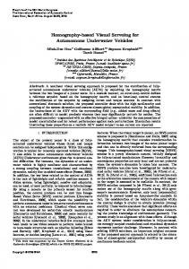
In this section we present some simulation results of the proposed visual servoing strategy. The desired position has been selected as cd = (0, 0, 0)
and Rd = I3 , and the initial one as cc = (−9, 1, 13)
and Rc = e[rc ]x with rc = (−π/2, π/2, −3π/10)
as shown in Figure 1. Observe that a large displacement and a large rotation are present between the two camera positions. The regions RA1 and RA2 have been selected as the boxes with corners (10, 10), (310, 10), (310, 190) and (10, 190) (for RA1), and (5, 5), (315, 5), (315, 195) and (5, 195) (for RA2) inside the image screen of size 320 × 200. The intrinsic parameters matrix K has been selected as   320 0 160   K =  0 200 100  . 0 0 1 The camera motion estimation has been performed through the essential matrix in both calibrated and uncalibrated cases using 8 point correspondences. Figure 2 shows, in the calibrated case, the translational motion (a), the rotational motion (b), the trajectory in the translational space (c) and the camera view during the visual servoing (d) obtained applying the proposed visual servoing. Notice that, since the camera is calibrated, the trajectory in the rotational space is guaranteed to be a straight line. Figure 3 shows the results obtained in the uncalibrated case selecting the estimate of K as   580 0 100  ˆ = K  0 350 80  . 0 0 1 Figure 3(d) shows the trajectory in the rotational space, and Figure 4 shows the camera trajectory in the 3D space. As we can see, the features are kept inside the field of view and the desired position is reached also in presence of large calibration errors. Observe that the trajectory of cc is quite far from the shortest one. This is due to the fact that, in some cases depending on the camera motion existing between initial and desired position and on the features displacement, to follow the shortest path in the rotational space does not allow to keep the features in the field of view by following a path in the translational space close to the shortest one. Indeed, a large use of the backward motion may be necessary to keep the features in the field of view while achieving the rotational convergence through the shortest path, which explains the non optimal trajectory in the translational space.

4

Conclusion

In this paper, a new visual servoing technique for steering a camera from a current to a desired position using point correspondences has been presented. This approach ensures, for known intrinsic 4

parameters and optical axis direction, global convergence and all points in the field of view of the camera during the robot control, without requiring any knowledge of the 3D model of the object and any path-planning. Moreover, the camera trajectory length is minimized in the rotational space and, for some cases including all the ones in which the features do not reach the image boundary, also minimized in the translational space. Robustness against uncertainty on the intrinsic parameters and optical axis direction is also guaranteed.

References [1] F. Chaumette. Potential problems of stability and convergence in image-based and positionbased visual servoing. In G. Hager D. Kriegman and A. Morse, editors, The confluence of vision and control, pages 66–78. Springer-Verlag, 1998. [2] P.I. Corke and S.A. Hutchinson. A new partitioned approach to image-based visual servo control. IEEE Trans. on Robotics and Automation, 17(4):507–515, 2001. [3] K. Deguchi. Optimal motion control for image-based visual servoing by decoupling translation and rotation. In Proc. Int. Conf. on Intelligent Robots and Systems, pages 705–711, 1998. [4] K. Hashimoto, editor. Visual Servoing: Real-Time Control of Robot Manipulators Based on Visual Sensory Feedback. World Scientific, Singapore, 1993. [5] K. Hashimoto, T. Kimoto, T. Ebine, and H. Kimura. Manipulator control with image-based visual servo. In Proc. IEEE Int. Conf. on Robotics and Automation, pages 2267–2272, 1991. [6] S. Hutchinson, G.D. Hager, and P.I. Corke. A tutorial on visual servo control. IEEE Trans. on Robotics and Automation, 12(5):651–670, 1996. [7] E. Malis and F. Chaumette. 2 1/2 D visual servoing with respect to unknown objects through a new estimation scheme of camera displacement. Int. Journal of Computer Vision, 37(1):79–97, 2000. [8] E. Malis, F. Chaumette, and S. Boudet. 2 1/2 D visual servoing. IEEE Trans. on Robotics and Automation, 15(2):238–250, 1999. [9] Y. Mezouar and F. Chaumette. Visual servoing by path planning. In Proc. 6th European Control Conference, pages 2904–2909, Porto, Portugal, 2001. [10] P. Oh and P. Allen. Visual servoing by partitioning degrees-of-freedom. IEEE Trans. on Robotics and Automation, 17(1):1–17, 2001. [11] C.J. Taylor and J.P. Ostrowski. Robust vision-based pose control. In Proc. IEEE Int. Conf. on Robotics and Automation, pages 2734–2740, San Francisco, California, 2000. [12] J. Weng, T.S. Huang, and N. Ahuja. Motion and structure from two perspective views: Algorithms, error analysis, and error estimation. IEEE Trans. on Pattern Analysis and Machine Intelligence, 11(5):451–476, 1989.

5

15

2 1.5

10

1

2

rotation [rad]

translation

5 0 −5

0.5 0 −0.5

−15 0

0

−2

1

2

3 time

4

5

−2 0

6

2

3 time

4

8

6

4

2

5

6

−10

0

x

(a) translational motion (cc components)

y axis

Figure 1: Example. Observed points and current and desired camera position.

1

1

0

0

−1 −2 −20

−10 x axis

2

−1 −2 0

0

(b) rotational motion (rc components)

10 z axis

z axis

z axis 2 1.5

0 x axis

2

0 x axis

2

1

0 −1

−0.5 z axis

0

0

10 5 0 −20

10

1

0 −2

20

15

15

2 y axis

10

z

−10 x axis

−0.5 −1 −2

0

(c) translational trajectory (cc components)

(d) rotational trajectory (rc components)

1 rotation [rad]

5 0 −5

0.5

200

0 −0.5

150

−10

−1

−15

−1.5

−20 0

1

2 time

3

v axis

translation

1

−5

y axis

12

−1.5

y axis

y

−1

−10

0

−2 0

4

1

2 time

3

100

4

50

(a) translational motion (cc components)

(b) rotational motion (rc components)

0 0

50

100

150 200 u axis

250

300

(e) camera view 200

2

−2 −4 −20

−10 x axis

0

0

−4 0

Figure 3: Example, uncalibrated case.

150

−2 10 z axis

20

v axis

0

y axis

y axis

2

100

10

50

5 0 −20

−10 x axis

0

(c) translational trajectory (cc components)

0 0

50

100

150 200 u axis

250

300

2

(d) camera view y

z axis

15

0

0 −5

−2 −10 12

10

8

6

4

2

0

−15 x

z

Figure 2: Example, calibrated case.

Figure 4: Example, uncalibrated case. Camera trajectory.

6