computer vision problems especially with multiple views. The Epipolar ... robot
SLAM is proposed in which the multiple view geometry is used to estimate the ...
The Epipolar Geometry Toolbox: multiple view geometry and visual servoing for MATLAB Gian Luca Mariottini and Domenico Prattichizzo Dipartimento di Ingegneria dell’Informazione, Universit`a di Siena Via Roma 56, 53100 Siena, Italy Email: {gmariottini,prattichizzo}@dii.unisi.it Abstract— The Epipolar Geometry Toolbox (EGT) was realized to provide a MATLAB user with an extensible framework for the creation and visualization of multi-camera scenarios and the manipulation of the visual information and the geometry between them. Functions provided, for both pin-hole and panoramic vision sensors, include camera placement and visualization, computation and estimation of epipolar geometry entities and many others. The compatibility of EGT with the Robotics Toolbox [7] allows to address general vision-based control issues. Two applications of EGT to visual servoing tasks are here provided. This article introduces the Toolbox in tutorial form. Examples are provided to show its capabilities. The complete toolbox, the detailed manual and demo examples are freely available on the EGT web site [21].
I. I NTRODUCTION The Epipolar Geometry Toolbox (EGT) is a toolbox designed for MATLAB [29]. MATLAB is a software environment, available for a wide range of platforms, designed around linear algebra principles and graphical presentations also for large datasets. Its core functionalities are extended by the use of many additional toolboxes. Combined with interactive MATLAB environment and advanced graphical functions, EGT provides a wide set of functions to approach computer vision problems especially with multiple views. The Epipolar Geometry Toolbox allows to design visionbased control systems for both pin-hole and central panoramic cameras. EGT is fully compatible with the well known Robotics Toolbox by Corke [7]. The increasing interest in robotic visual servoing for both 6DOF kinematic chains and mobile robots equipped with pin-hole or panoramic cameras fixed to the workspace or to the robot, motivated the development of EGT. Several authors, such as [4], [9], [18], [20], [24], have proposed new visual servoing strategies based on the geometry relating multiple views acquired from different camera configurations, i.e. the Epipolar Geometry [14]. In these years we have observed the necessity to develop a software environment that could help researchers to rapidly create a multiple camera setup, use visual data and design new visual servoing algorithms. With EGT we provide a wide set of easy-to-use and completely customizable functions to design general multi-camera scenarios and manipulate the visual information between them.
Let us emphasize that EGT can also be successfully employed in many other contexts when single and multiple view geometry is involved as, for example, in visual odometry and structure from motion applications [23] [22]. For example in the first work an interesting “visual odometry” approach for robot SLAM is proposed in which the multiple view geometry is used to estimate the camera motion from pairs of images without requiring the knowledge of the observed scene. EGT, as the Robotics Toolbox, is a simulation environment, but the EGT functions can be easily embedded by the user in Simulink models. In this way, thanks to the MATLAB RealTime Workshop, the user can generate and execute stand-alone C code for many off-line and real-time applications. A distinguishable remark of EGT is that it can be used to create and manipulate visual data provided by both pinhole and panoramic cameras. Catadioptric cameras, due to their wide field of view, has been recently applied in visual servoing [32]. The second motivation lead to the development of EGT was the increasing distribution of “free” software in the latest years, on the basis of the Free Software Foundation [10] principles. In this way users are allowed, and also encouraged, to adapt and improve the program as dictated by their needs. Examples of programs that follow these principles include for instance the Robotics Toolbox [7], for the creation of simulations in robotics, and the Intel’s OpenCV C++ libraries for the implementation of computer vision algorithms, such as image processing and object recognition [1]. The third important motivation for EGT was the availability and increasing sophistication of MATLAB. EGT could have been written in other languages, such as C, C++ and this would have freed it from dependency on other software. However these low-level languages are not so conducive to rapid program development as MATLAB. This tutorial assumes the reader has familiarity with MATLAB and presents the basic EGT functions, after short theory recalls, together with intuitive examples. In this tutorial we also present two applications of EGT to visual servoing. Section 2 presents the basic vector notation in EGT, while in Section 3 the pin-hole and omnidirectional camera models together with EGT basic functions are presented. In Section 4 we present the setup for multiple camera geometry (Epipolar
xc
yc Xc
θ zc
zw
Xw
CCD
Xm
Consider now the more general case in which two camera frames, referred to as actual and desired, are observing the same point Xw . From (1)
yw
Oc φ
c tw ;
ψ
c Rw
xw
Ow
ym
xm
World frame Sw
xc
yc
Om
(3)
Xw
Raw Xa
(4)
=
T
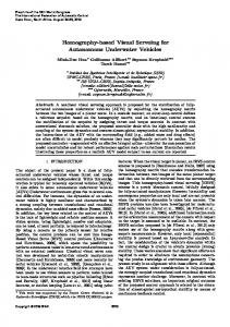
Main reference frames notation and vector representation in EGT.
Geometry) while in Section 5 two applications of EGT to visual servoing are presented together with simulation results. In Section 6 we make a comparison between EGT and other software packages. EGT can be freely downloaded at [21], can be used under Windows and requires MATLAB 6.5 or upper. The detailed manual is provided in the EGT web site, with a large set of examples, figures and source code also for beginners. VECTOR NOTATION
We here present the basic vector notation adopted in Epipolar Geometry Toolbox. All scene points Xw ∈ IR3 are expressed in the world frame Sw =< Ow xw yw zw > (Fig.1). When referred to the pin-hole camera frame Sc =< Oc xc yc zc > they will be indicated with Xc . Moreover all scene points expressed w.r.t. a central catadioptric camera frame Sm =< Om xm ym zm > will be indicated with Xm . For the reader convenience we briefly present the basic vector notation and transformation [25]. Refer to Fig. 1 and consider the 3×1 vector Xc ∈ Sc . It can be expressed in Sw as follows: Xw = Rcw Xc + tcw
= Rdw Xd + tdw +
Xd = Rdw Raw Xa + Rdw | {z } |
Central Catadioptric Camera frame Sm
II. BASIC
Xw
taw
Substituting (4) in (3) it follows
zm
Pin-hole Camera frame Sc
Fig. 1.
zc
(1)
where tcw is the translational vector centered in Sw and pointing toward the Sc frame (Fig. 1). The matrix Rcw is the rotation necessary to align the world frame with the camera frame. For example we may choose Rcw = Rroll,pitch,yaw = Rz,θ Ry,φ Rx,ψ . The homogeneous notation aims to express (1) in linear form: e w = Hc X ec X
Ra d
Analogously, a point Xw can be expressed in the camera frame by the following transformation � � cT Rw −Rcw T tcw ˜ e Xw (2) Xc = 0T 1
� taw − tdw {z }
(5)
ta d
Equation (5) will be very useful in EGT for the analytical computation of epipolar geometry where it is necessary to know the relative displacement tad and orientation Rad between the two camera frames. III. P IN - HOLE AND
OMNIDIRECTIONAL CAMERA MODELS
EGT provides easy-to-use functions for the placement of pin-hole and central catadioptric (or omnidirectional) cameras. Their imaging model has been here implemented to allow users to manipulate the visual information. In this section the fundamentals of perspective and omnidirectional camera models are quickly reviewed. The reader is referred to [14], [17], [5] for a detailed treatment. According to the purposes of this tutorial, some basic EGT code examples are reported together with the theory. A. Perspective camera Consider a pin-hole camera located at Oc as in Fig. 2. The full perspective model describes the relationship between a 3D point (in homogeneous coordinates) � � e w = X Y Z 1 T expressed in the world frame and X � �T ˜ = u v 1 its projection m onto the image plane according to ew e = KΠX m where K ∈ IR3×3 is the camera intrinsic parameters matrix given by: ku f γ u0 K= 0 kv f v0 . 0 0 1 Image plane coordinates
(0,0)
u
Optical Axis
u0
v
w
e c = [Xc T 1]T . The 4 × 4 matrix e w = [Xw T 1]T , X where X c Hw is referred to as homogeneous transformation matrix: � c � Rw tcw Hcw = 0T 1
T
v0
Xc
Xw zw
m
yw
f
Ow
zc
World frame coordinates
Oc yc
xw
xc
Camera-centered coordinates
I (R,t)
Fig. 2. The pin-hole camera model. The 3D point Xw is projected onto m through the optical center Oc . Note that m is expressed in the image plane coordinates (u, v) (pixels).
3D setup EGT Tutorial Ex.1
In order to directly obtain the 4 × 4 homogeneous matrix Hw c the function f_Rt2H is provided >> H=f_Rt2H(R,t).
Note that with the use of f_Rt2H the position t of a pin-hole camera is specified with respect to the world frame while the rotation R is referred to the pin-hole camera frame axes. During the testing phase at the University of Siena this choice was appreciated from students of Robotics and Vision classes that addressed it as very intuitive. Example 1 (3D scene and pin-hole camera placement): Consider now a pin-hole camera rotated by R = Ry,π/4 ∈ IR3×3 and translated by t = [−10, −5, 0]T : >> R=rotoy(pi/4); >> t=[-10,-5,0]’; >> H=f_Rt2H(R,t); In EGT the camera frame and the associated 3D camera can be visualized with functions f_3Dframe(H) and f_3Dcamera(H) respectively, where H is the 4×4 homogeneous transformation describing position and orientation of the camera with respect to Sw >> >> >> >> >>
f_3Dframe(H,1); %camera frame hold on f_3Dcamera(H); %3D pin-hole camera axis equal, grid on, view(12,34) title(’3D setup - EGT Tutorial - Ex.1’)
Plot of 3D view is reported in Fig. 3(a). All the functions have further options. See the EGT Manual [21] for details. We can also place a set of N 3D points Xiw = [X i , Y i , Z i ] (e.g. the rectangular panel vertexes) defined as 1 X X2 . . . XN Xw = Y 1 Y 2 . . . Y N ∈ IR3×N Z1 Z2 . . . ZN
0.3
Image Plane EGT Tutorial Ex.1 4 3
0.2 4
Zwf
3
0.1
Ywf
0
5
Zc
1
2
X
wf
0.1 Zm
Here (u0 , v0 ) are the pixels coordinates, in the image frame, of the principal point (i.e. the intersection point between the image plane and the optical axis zc ), ku and kv are the number of pixels per unit distance in image coordinates, f is the focal length (in meters) and γ is the orthogonality factor of the CCD image axes (skew-factor). Matrix Π = [R | t] ∈ IR3×4 is the so-called external parameters camera matrix, that contains the rotation R and the translation t between the world and the camera frames. According to the commonly used notation, in the case of no camera rotation the optical axis zc of pin-hole cameras is parallel to the yw axis of Sw . We then define: �T R = Rx,−π/2 Rrpy �T t = − Rx,−π/2 Rrpy tcw
0
4
Xc
2
-2 -4
-5 -12
- 10
-8
0.2
2
0
Yc
Ym
0.3
1
-6 -6
-4 Xm
-2
0
-8 2
0.4 0.1
0.05
0
0.05
0.1
0.15
0.2
0.25
4
(a)
(b)
Fig. 3. Example 1. (a) A pin-hole camera is positioned in t = [−10, −5, 0] in the 3D world frame and rotated by π/4 around the y-axis. (b) The 3D scene points are projected onto the image plane. Note that in this case K = I for simplicity.
by the use of function f_scenepnt(X) >> >> >> >> >> >>
Xi=[-3, 3, 3, -3]; Yi=[ 3, 3, 3, 3]; Zi=[-3, -3, 3, 3]; Xw=[Xi; Yi; Zi]; f_scenepnt(Xw); f_3Dwfenum(Xw); %enumerate points
The perspective projection m = [u, v]T of points Xw is obtained with f_perspproj(Xw,H,K): >> [u,v]=f_perspproj(Xw,H,K); >> plot(u,v,’rO’) Projection of scene points is represented in Fig. 3(b). � Note that while the above example describes the placement of 3D points Xw , EGT is also able to build scenes with more complex 3D objects returning surface points and normals (see function f_3Dsurface in [21]). B. Omnidirectional Camera Model Omnidirectional cameras combine reflective surfaces (mirrors) and lenses. Several types of panoramic cameras can be obtained simply combining cameras (pin-hole or orthographic) and mirrors (hyperbolic, parabolic or elliptical) [5]. Panoramic cameras are classified according to the fact that they satisfy or not the single viewpoint constraint guaranteeing that the visual sensor only measures the light through a single point. Note that this constraint is required for the existence of epipolar geometry and for the generation of geometrically correct images [28] [12]. In [3], Baker et al. derive the entire class of catadioptric systems verifying the single viewpoint constraint. Among these EGT takes into account catadioptric systems consisting of pin-hole cameras coupled with hyperbolic mirrors, and orthographic cameras coupled with parabolic mirrors. In [11] a unified projection model for central catadioptric camera systems has been proposed. In particular it was shown that all central panoramic cameras can be modelled by a
X zm Hyperbolic mirror
ym
xm
Om
In EGT a central catadioptric camera is defined by specifying the homogeneous transformation matrix between mirror and world frames � m m � Rw tw Hm = w 0T 1
Xw
Xh Xc
zw yw xw Ow
Example 2 (Panoramic camera placement): In EGT a panoramic camera can be placed and visualized. Let us place the camera at t=[-5,-5,0]’ with orientation R≡ Rz,π/4 . EGT provides a function to simply visualize the panoramic camera in the 3D world frame as in Fig. 5.
2e
m zc f
>> H=[rotoz(pi/4) , [-5,-5,0]’; >> 0 0 0 , 1 ]; >> f_3Dpanoramic(H);
xc
Fig. 4. The panoramic camera model (pin-hole camera and hyperbolic mirror). The 3D point Xw is projected at m through the optical center Oc , after being projected at Xh through the mirror center Om .
particular mapping on a sphere, followed by a projection from a point on the camera optical axis onto the image plane. In order to keep in EGT a physically meaningful graphical representation we decided, without loosing generality, to represent the central panoramic cameras not as spheres in the space but with the couple of a CCD camera with a parabolic or hyperbolic mirror (see for example Fig. 5). In what follows the imaging model for a pin-hole camera with hyperbolic mirror is described. Consider now the basic scheme in Fig. 4. Note that in this case all frames (for both the camera and the mirror) are aligned with the world frame. Three important reference frames are defined: (1) the world reference system centered at Ow whose vector is Xw ; (2) the mirror coordinate system centered at the focus Om whose vector is X = [X, Y, Z]T ; and (3) the camera coordinate system centered at Oc whose vector is Xc . Henceforth all equations will be expressed in the mirror reference frame if not stated otherwise. Refer to Fig. 4 and let a and b be the hyperbolic mirror parameters (z + e)2 x2 + y 2 − =1 2 a b2 √ with eccentricity e = a2 + b2 , the transformation to obtain the projection u in the pin-hole camera frame (see Fig. 4) is given by � � 1 � m � mT m ) + t Rc λRw (Xw − tm m=K w c 2e b2 (−eZ±a||X||) b2 Z 2 −a2 X 2 −a2 Y 2
Moreover, for assigned camera calibration matrix K: K=[10ˆ3 0 0 10ˆ3 0 0
the projection of a 3D point Xw=[0,0,4]’ in both the camera (m) and mirror (Xh) frames can be obtained from: >> [m,Xh] = f_panproj(Xw,H,K); >> m = 4.1048e+002 2.4000e+002 1.0000e+000 Xh = 6.0317e-001 3.7881e-017 3.4120e-001 EGT - Central Catadioptric Imaging of 3D scene points
6
4
EGT CCD Panoramic Camera Plane 240.5 2
X
w
Z
Z
c
wf
0
Y
c
Xh
X
-2
Y
c
wf
X
wf
-4
m
240
Z
-6
c
(6)
where λ = is a nonlinear function of X. K is the internal calibration matrix of CCD camera looking at the mirror. tm c is the mirror center expressed in the camera frame and corresponds to [0, 0, 2e]. Rm c is the matrix representing the rotation between camera and mirror frames. Analogously m tm w and Rw represent the mirror configuration (rotation and orientation) with respect to the world frame.
320; 240; 1 ];
v [pixels]
yc Oc
Zm
Pin-hole camera
Y
c
X
239.5
c
-6 -4 Xm -2
410
410.2 410.4 410.6 410.8 u [pixels]
411
0 2 -6
-4
-2
0
2
Ym
(a)
(b)
Fig. 5. Example 2. (a) A panoramic camera is positioned in [−5, −5, 0]T in the 3D world frame and (b) the 3D point Xw = [0, 0, 4]T is projected to the pinhole camera after being projected in Xh .
Basic epipolar geometry setup
Xw
I2 1
X
l2
I1 m2 m1
O1 ya
e1
za
X
10
zd
baseline
e2
xd
O2 yd
2
5 Zm
l1
Zd
0 Z
a
xa
5
Xd
X Yaa
Yd
(R,t)
10
15
Fig. 6.
5
10
Basic Epipolar Geometry entities for pinhole cameras.
0
5 0
Xm
Ym
5 5
10 10
1.0000e+000
(a) Image plane for pinhole camera in O1
Image plane for pinhole camera in O 2 0.1
0.5
e
2
0
e 0
v [pixel]
0.1
v [pixel]
Graphical results are reported in Fig. 5 and more accurately described in the EGT Reference Manual. More examples can be found in the directory demos. �
0.5
0.2
0.3
0.4
1 m
m 2
1
1
1
0.5 2 1
m m
2
2
1.5
IV. E PIPOLAR G EOMETRY In this section the EGT functions dealing with the Epipolar Geometry are presented. A. Epipolar geometry for pin-hole cameras Consider two perspective views of the same scene taken from distinct viewpoints O1 and O2 , as in Fig.6. Let m1 and m2 be the corresponding points in two views, i.e. the perspective projection through O1 and O2 , of the same point Xw , in both image planes I1 and I2 , respectively. The epipolar geometry defines the geometric relationship between these corresponding points. Associated with Fig.6 we define the following set of geometric entities [14], [17]: Definition 1: Epipolar Geometry 1) The plane passing through the optical centers O1 and O2 and the scene point Xw , is called an epipolar plane. Note that in a N -points scene, a pencil of planes exists (one for each scene point Xiw ) 2) The projection e1 (e2 ) of one camera center O1 (O2 ) onto the image plane of the other camera frame I2 (I1 ) is called epipole. The epipole will be expressed in homogeneous coordinates � �T � �T ˜1 = e1x e1y 1 ˜2 = e2x e2y 1 e e
3) The intersection of the epipolar plane for Xw with image plane I1 (I2 ), defines the epipolar line l1 (l2 ). Note that all epipolar lines pass through the epipole. One of the main parameters of the epipolar geometry is the 3×3 Fundamental Matrix F that conveys most of the information about the relative position and orientation (t, R) between the two views. Moreover, the fundamental matrix
0.6
2
1.5
1
0.5
0
0.5
1
1
0.9
0.8
0.7
0.6
0.5
0.4
0.3
0.2
0.1
0
u [pixel]
u [pixel]
(b)
(c)
Fig. 7. Example 3. (a) 3D simulation setup for epipolar geometry, with both cameras looking at two scene points X1w and X1w ; (b)-(c) image planes of both pin-hole cameras with corresponding features and epipoles. Note that all epipolar lines meet at the epipole and pass through the corresponding points.
algebraically relates corresponding points in the two images through the Epipolar Constraint: Theorem 1: (Epipolar Constraint) Let be given two views of the same 3D point Xw , both characterized by their relative position and orientation (t, R) and the internal calibration parameters K1 and K2 . Moreover, let m1 and m2 (homogeneous notation) be the two corresponding projections of Xw in both image planes. The epipolar constraint is: mT2 Fm1 = 0
where
F = K2 −T [t]× RK1 −1 .
and [t]× is the 3 × 3 skew-symmetric matrix associated to t. � The epipolar geometry is reviewed extensively in [14], [17]. Example 3 (Epipolar Geometry for pinhole cameras): The computation of epipolar geometry with EGT is straightforward. Consider a two-views scene as in Fig. 7(a) where the first camera is placed at t1 = [−10, −10, 0]T with orientation R1 = Ry,π/4 , while the second one is coincident with the world frame, i.e. t2 = [0, 0, 0]T with orientation R2 = I. Pin-hole cameras can be shown and their homogeneous transformation matrices H1 and H2 can be obtained with f_Rt2H as described in Sec. III-A. Two feature points in X1w = [0, 10, 10]T and X2w = [−10, 5, 5]T are observed and projected in m11 , m21 and m12 , m22 onto the
two image planes, respectively. In EGT the computation of epipoles and fundamental matrix is obtained through function
with the baseline Om1 Om2 (see Fig.8). 7 3
>> [e1,e2,F]=f_epipole(H1,H2,K1,K2); 8
while the epipolar lines are retrieved with:
4
15
6
>> [l1,l2]=f_epipline(m1,m2,F);
2
10
B. Epipolar Geometry for panoramic cameras
5 5
Yc
1
Zm
Note that l1 (l2 ) is a vector in IR3 in homogeneous coordinates. In (Fig. 7(b)) both image planes are represented together with feature points, epipoles and the corresponding epipolar lines. In this case, for the sake of simplicity, it is assumed that K = I.
Yc Xc
Xc Zwf
Zc
0
Ywf
Yc e1ad Xc
-5
e2ad
X wf Yc e1da Xc
Zc e2da Zc
Z
c
As in the pinhole cameras, the epipolar geometry is here defined when a pair of panoramic views is available. Note however that in this case epipolar lines become epipolar conics. The reader is referred to [11], [27] for an exhaustive treatment. Let now consider two panoramic cameras (with equal hyperbolic mirror Q) with foci Om1 and Om2 respectively, as represented in Fig. 8. Moreover, let be R and t be the rotation and translation between the two mirror frames, respectively. Let Xh1 and Xh2 represent the mirror projections of the scene point X onto both hyperbolic mirrors. The coplanarity of Xh1 , Xh2 and X can be expressed as: XTh2 EXh1 = 0
where
E = [t]× R
(7)
Equivalently to the pin-hole case, the 3×3 matrix E is referred to as the essential matrix [15]. Vectors Xh1 , Xh2 and t define the epipolar plane with normal vector nπ , that intersects both mirror quadrics Q in the two epipolar conics C1 and C2 [26]. For each 3D point Xi a pair of epipolar conics Ci1 and Ci2 exist for the two views setup. All the epipolar conics pass through two pairs of epipoles, e1 and e′1 for one mirror and e2 and e′2 for the second one, which are defined as the intersections of the two mirrors Q
X nπ m2
m1
Xh1
e1
e1'
baseline
Om1
C1
Fig. 8.
(R , t ) Q
e2
Xh2 Om2
C2
Epipolar geometry for panoramic camera sensors.
e2'
15 5
10
(D) 5 Ym
0
(A) 0
-5
Xm
-5
Fig. 9. Example 4: Central catadioptric cameras: epipolar geometry computation and visualization in EGT.
Example 4 (Epipolar geometry for panoramic cameras): Similar camera and scene configurations as for the Example 3 have been set. Now we placed 8 feature points in the space. By using the EGT function: >> [e1c,e1pc,e2c,e2pc] = f_panepipoles(H1,H2);
the CCD coordinates of the epipoles are easily computed and plotted. The CCD projections of all epipolar conics Ci1 and Ci2 where i = 1, ..., 8, corresponding to all 3D points in Xw are computed and visualized by >> [C1m,C2m] = f_epipconics(Xw,H1,H2); � Fig. 9 presents the application of EGT to the computation of epipolar geometry between central catadioptric cameras (A) and (D). Note that also the epipoles onto the mirror surface are visualized. Epipolar conics in both CCD image plane, together with corresponding feature points, are showed in Fig. 10(A)-(B). The complete MATLAB source code is available at the EGT web-site [21]. C. Estimation of Epipolar Geometry
Q
Up to now the EGT functions we presented for the epipolar geometry computation were based on the knowledge of the relative position and orientation between the two cameras. However many algorithms exist in the literature to estimate
feature points
feature points
The visual servoing controllers proposed by Rives in [24] (for pin-hole cameras) and that proposed in [19] (for central panoramic cameras) have been considered as tutorial examples to show the main EGT features in a visual servoing context.
epipole epipole
0
0
epipole
epipole 0.05 v [pixels]
v [pixels]
0.05 0.1 0.15
0.1 0.15
A. Visual Servoing with Pin-hole Cameras for 6DOF Robots
epipolar conics
0.2
0.2 0.1
0 u [pixels]
0.1
0.2
0.05
0
0.05 0.1 u [pixels]
0.15
0.2
(B)
(A)
Fig. 10. Example 4: Epipolar conics plot in camera planes (A) and (B). All epipolar conics, in each image plane, intersect at the epipoles.
ID 1 2 3
Estimation Algorithm Unconstrained linear estimation [16] The normalized 8-point algorithm [13] Algorithm based on Geometric Distance (Sampson) [14]
TABLE I T HE EPIPOLAR GEOMETRY ESTIMATION ALGORITHMS IMPLEMENTED IN EGT ( WITH BIBLIOGRAPHY ).
the epipolar geometry from the knowledge of corresponding feature points mia and mid . A very important feature of EGT is that some of the most important algorithms for the epipolar geometry estimation have been embedded in the toolbox code. In particular we implemented the linear method [16], the well known Hartley’s normalized 8-points algorithm [13] and the iterative algorithm based on geometric distance (Sampson) [14] as summarized in Table I. A complete comparison and review of these methods has been reported in [14]. The epipolar geometry estimation is one of the most relevant features of EGT. The main reason is that users can run simulations where the fundamental matrix is estimated from noisy feature points. The basic EGT function to estimate the fundamental matrix F is
In what follows the algorithm proposed in [24] is briefly recalled for the reader convenience. The main goal of this visual servoing is to drive a 6DOF robot arm (simulated with RT), equipped with a CCD camera (simulated with EGT), from a starting configuration toward a desired one using only image data provided during the robot motion (Fig. 11). The basic visual servoing idea consists in decoupling the camera/endeffector rotations and translations by the use of the hybrid vision-based task function approach [9]. The servoing task is performed minimizing an error function ϕ which is divided in both a priority task ϕ1 , that acts rotating the actual camera until the desired orientation is get, and in a secondary task ϕ2 (to be minimized under the constraint ϕ1 = 0) that has been chosen in [24] to be the camera distance to the target position. The analytical expression of the error function is given by ϕ = W + ϕ1 + β(II6 −W + W )
∂ϕ2 ∂X
(8)
where β ∈ IR+ , while W + is the pseudo-inverse of the matrix W ∈ IRm×n : Range(W T ) = Range(J1T ) where J1 is the 1 Jacobian matrix of task function J1 = ∂ϕ ∂X . The priority task accomplishes to rotate the camera/endeffector using a well-known epipolar geometry property stating that when both the initial and the desired cameras gain the same orientation, then all the distances between feature points mi and corresponding epipolar lines l′i are zero.
>> F=f_Festim(U1,U2,algorithm); where U1 and U2 are two (2 × N ) matrices containing all N corresponding features � 1 � x1 x21 ... xN 1 U1 = y11 y12 ... y1N
zy x
The integer algorithm identifies the type of estimation algorithm to be used between those available according to Table I. It is worth noting that these functions allows EGT to estimate the epipolar geometry also in real experiments other than simulations. V. V ISUAL S ERVOING When used together with a robotics toolbox, such as the Robotics Toolbox (RT) by Corke [7], EGT proves to be an efficient tool to implement visual servoing techniques based also on multiple view geometry.
Fig. 11. Simulation setup for EGT application to visual servoing. EGT is compatible also with Robotics Toolbox.
Desired Image Plane
0.7
< Oxyz >w (Fig. 14). Let vx ,vy be the translational velocities and ω the rotational velocity, respectively
starting point
x˙ = vx y˙ = vy θ˙ = ω
0.6 0.5 0.4
(9)
target point 0.3 epipolar line
0.2 0.1 0 0.1 0.2 0.3 0.8
0.6
0.4
0.2
0
0.2
0.4
Fig. 12. Migration of feature points from initial position toward desired one. Feature points, from a starting position, reach the epipolar lines at the end of the first task (priority task) and then move toward desired ones (crossed points), during the second task. 1.5
ω x ω y ω z v x v y v
0.16
0.14
0.12
Norm of the error
Control inputs
1
z
0.5
0
0.1
0.08
β=0
0.06
0.04 0.5
0.02
β=1
0
1 0
20
40
60
80
100
120
samples
140
160
180
200
20
40
60
80
100
120
140
160
180
200
samples
Fig. 13. (a) Control inputs to PUMA 560; (b) Norm of the error function e when β = 0 and when β = 1.
Fig. 12 shows the simulation results of the algorithm previously proposed for a scene with 8 points. The dotted points in Fig. 12 shows, in the image plane (K = I), the migration of the features to the epipolar lines during the rotation (first task), while crossed points correspond to the camera translation (second task). In Fig. 13 the control inputs (vc , ωc ) and the plot of the norm of the error function e are reported. The MATLAB code of this simulation (SIM_Rives00.m) is included in the directory demo_pinhole of EGT [21].
Suppose that a fixed catadioptric camera is mounted on the mobile robot such that its optical axis is perpendicular to the xy-plane. Without loosing generality, suppose that a target panoramic image, referred to as desired, has been previously acquired in the desired configuration qd = (0, 0, 0)T . Moreover, one more panoramic view, the actual one, is available at each time instant from the camera-robot in the actual position. As shown in the initial setup of Fig. 15 (upper-left), the mobile robot disparity between the actual and the desired poses is characterized by rotation R ∈ SO(2) and translation t ∈ IR2 . The control law will be able to drive the robot disparity between the actual and the desired configuration to zero only using visual information. In particular, we will regulate separately the rotational disparity (first step) and the translational displacement (second step) (upper-center and upper-right in Fig. 15, respectively). In the first step the rotational disparity is compensated exploiting the auto-epipolar condition [19]. This novel property is based on the concept of bi-osculating conics (or bi-conics, for short), computed on the image plane from observed image corresponding features. It has been shown [19] that when all bi-conics intersect in only two points then the rotational disparity between the actual and the desired view is compensated. Fig. 15 (bottom-left) shows the image plane bi-conics when the two cameras are not in auto-epipolar configuration. On the other hand Fig. 15 (bottom-center) shows the image plane bi-conics when the cameras are in auto-epipolar configuration and all bi-conics intersect in only two points. Once the rotational disparity is compensated, then the second step is executed. It consists of a translational motion in which the robot is constrained to move along the baseline in order to approach the desired position (Fig. 15 top-right). This translational control law can be designed on the image plane constraining all current features to lie on the epipolar conics and also the distance between current and desired features s(t)
B. Visual Servoing with Panoramic Cameras for Mobile Robot While visual servoing with pin-hole cameras has been deeply investigated in the literature, less results exist for omnidirectional cameras. Interesting contributions for mobile robots equipped with panoramic cameras can be found in [6], [8], [31]. We here briefly recall the application of the Epipolar Geometry Toolbox to the design of a visual servoing technique for holonomic mobile robots equipped with a central panoramic camera presented in [19]. The proposed strategy does not assume any knowledge about the 3D observed scene geometry and position with respect to the camera/robot. Consider a holonomic mobile robot and let q = (x, y, θ)T be its configuration vector with respect to the world frame
[v x ,v y ] ω y
x θ
y(t)
0
x (t)
Fig. 14. The holonomic mobile robot with a fixed catadioptric camera moving on a plane.
ω ca1
y(0)
ca1
y(t)
fa
fa
θ
ca2
ca2 ca1
y(t) ba se lin
e
fa
ba se lin
e
ca2
v =[v x ,v y ]
cd1
cd1
cd1
fd
fd
x (0)
cd2
fd
x (t)
First Step Auto -epipolar Configuration
Starting Configuration
x (t)
cd2
cd2
Second Step Translational motion
Desired features
s(t)
Actual features
Fig. 15. The visual servoing control law for panoramic cameras drives the holonomic camera-robot from the starting configuration centered at fa (no common intersection between bi-conics exists), through an intermediate configuration when both views have the same orientation (bi-conic common intersection), towards the position fd (until s(t) = 0). Bottom figures have been obtained with EGT.
10
15
5
5 8
0
5
-5
7
4
3
1
2
Zm
Zm
10
Y
c
6
10
5
Y
c
X
c
10 0 -10
-10
0
-5
10
5 Xm
Ym 5
15
0 -5
3D camera setup - Actual camera configuration
-10
-5
0
15
10
5 Xm
3D camera setup -- Desired camera configuration
0.14
0.06 0.04
6 1
5 8
2
7 4
0.12 0.1 ω [rad/sec.]
0 3 2 74 61 8 5
VI. C OMPARISON
0.08
0.02
-0.02
0
0.02
0.04
WITH OTHER PACKAGES
0.06 0.04
-0.04
-0.04
the epipolar conics. In the right bottom Fig. 16 it is shown the angular velocity ω provided by the controller that decreases to zero. Fig. 17 shows simulation results for the second step. In the left-top window the translational velocities vx (t) and vy (t) are reported. In the right-top window the distance s(t) between all feature points goes to zero, as reported in the bottom center window, where crossed points (actual positions) go to the desired one (circles). The MATLAB code for the auto-epipolar property is the ex5_autoepipolar.m and is included in the directory demo_panoramic of EGT.
3
0.02
-0.06 -0.06
2
6
-5
c
-0.02
1 8
-10 15
Y
Ym
3
7
0
X
c
4
0.06
Rotational Controller - Motion of features to the epipolar conic-
0
0
5
10
15 t [sec.]
20
25
30
Rotational Controller - Angular velocity
Fig. 16. Simulation results with EGT for the first step. The robot, placed in the actual configuration, rotates until the same orientation of the desired configuration is obtained.
to decrease as the robot approach the goal (Fig. 15 bottomright). Fig. 16 gathers some simulation results for the first step. The left and the right top windows show, respectively, the actual and desired camera locations, together with scene points. On the left bottom window of Fig. 16 we can observe the feature points (crosses) moving from initial position towards
To the best of our knowledge no other software packages for the MATLAB environment exist that deal with the creation of multi-camera scenarios for both pin-hole and panoramic cameras. An interesting MATLAB package is the Structure and Motion Toolkit by Torr [30]. This toolkit is specifically designed for features detection and matching, robust estimation of the fundamental matrix, self-calibration, and recovery of the projection matrices. The main difference with EGT is that the work of Torr is specifically oriented to pin-hole cameras and is not specifically designed to run simulations. Regarding the visual servoing, it is worthwhile to mention the interesting Visual Servoing Toolbox (VST) by Cervera et al. [2] providing a set of Simulink blocks for simulation of vision-controlled systems. The main difference is that the VST implements some well known visual servoing control laws but does not consider neither multiple view geometry
0
0.2 v x v
-0.1
0.18
y
0.16 0.14
-0.4 -0.5
0.12
s(t) [pixels]
y
-0.3
x
v and v [m/sec]
-0.2
0.1 0.08 0.06
-0.6
0.04 -0.7 -0.8
0.02 0
20
40 t [sec.]
60
0
80
0
10
20
30
40
50
t [sec.]
Translational controller - velocities
Translational controller - Distance s(t)
0.06 6 1
5
0.04
8 0.02 0
2
7 4
3
2 6 1 7 3 5 84
-0.02 -0.04 -0.06 -0.06
-0.04
-0.02
0
0.02
0.04
0.06
Translational Controller - Motion of features
Fig. 17. Simulation results with EGT for the second step. The translational controller guarantees the motion of the robot along the baseline (the feature slide along the bi-conic). Then it stops when the distance s(t) between corresponding features is equal to zero i.e. the robot is in the desired pose.
nor panoramic cameras that are the distinguishing features of EGT. VII. C ONCLUSIONS The Epipolar Geometry Toolbox for MATLAB is a software package targeted to research and education in Computer Vision and Robotics Visual Servoing. It provides the user a wide set of functions for design multi-camera systems for both pin-hole and panoramic cameras. Several epipolar geometry estimation algorithms have been implemented. EGT is freely available and can be downloaded at the EGT web site together with a detailed manual and code examples. VIII. ACKNOWLEDGMENTS Authors want to thank Eleonora Alunno for her help to develop EGT functions during her Master Thesis and to Jacopo Piazzi for his useful comments. EGT has been widely tested by the students of the Robotics and Vision classes and laboratories at the University of Siena who contributed to the testing phase of Epipolar Geometry Toolbox. Special thanks go to Paola Garosi, Annalisa Bardelli and Fabio Morbidi that helped us with useful comments on the toolbox and on the paper. R EFERENCES [1] Intel’s OpenCV. http://sourceforge.net/projects/opencvlibrary/. [2] The Visual Servoing Toolbox, 2003. http://vstoolbox.sourceforge.net/. [3] S. Baker and S.K. Nayar. Catadioptric image formation. In Proc. of DARPA Image Understanding Workshop, pages 1431–1437, 1997. [4] R. Basri, E. Rivlin, and I. Shimshoni. Visual homing: Surfing on the epipoles. In International Conference on Computer Vision, pages 863– 869, 1998. [5] R. Benosman and S.B. Kang. Panoramic Vision: Sensors, Theory and Applications. Springer Verlag, New York, 2001.
[6] D. Burschka and G. Hager. Vision-based control of mobile robots. In 2001 IEEE International Conference on Robotics and Automation, pages 1707–1713, 2001. [7] P.I. Corke. A robotics toolbox for MATLAB. IEEE Robotics and Automation Magazine, 3:24–32, 1 1996. [8] N. Cowan, O. Shakernia, R. Vidal, and S. Sastry. Vision-based follow the leader. In 2003 IEEE/RSJ International Conference on Intelligent Robots and Systems, volume 2, pages 1796–1801, 2003. [9] B. Espiau, F. Chaumette, and P. Rives. A new approach to visual servoing in robotics. In IEEE Transactions on Robotics and Automation, volume 8(3), 313–326 1992. [10] Free Software Foundation. The free software definition. http://www.fsf.org/philosophy/free-sw.html. [11] C. Geyer and K. Daniilidis. A unifying theory for central panoramic systems. In 6th European Conference on Computer Vision, pages 445– 462, 2000. [12] C. Geyer and K. Daniilidis. Mirrors in motion: Epipolar geometry and motion estimation. In 9th IEEE International Conference on Computer Vision, volume 2, pages 766–773, 2003. [13] R. Hartley. In defence of the 8-point algorithm. In IEEE International Conference on Computer Vision, pages 1064–1070, 1995. [14] R. Hartley and A. Zisserman. Multiple view geometry in computer vision. Cambridge University Press, September 2000. [15] H.C. Longuet-Higgins. A computer algorithm for recostructing a scene from two projections. Nature, 293:133–135, 1981. [16] Q.T. Luong and O.D. Faugeras. The fundamental matrix: theory, algorithms and stability analysis. International Journal of Computer Vision, 17(1):43–76, 1996. [17] Y. Ma, S. Soatto, J. Koˇseck´a, and S. Shankar Sastry. An invitation to 3-D Vision, From Images to Geometric Models. Springer Verlag, New York, 2003. [18] E. Malis and F. Chaumette. 2 1/2 d visual servoing with respect to unknown objects through a new estimation scheme of camera displacement. International Journal of Computer Vision, 37(1):79–97, 2000. [19] G.L. Mariottini, E. Alunno, J. Piazzi, and D. Prattichizzo. Epipolebased visual servoing with central catadioptric camera. In 2005 IEEE International Conference on Robotics and Automation, 2005. (in press). [20] G.L. Mariottini, G. Oriolo, and D. Prattichizzo. Epipole-based visual servoing for nonholonomic mobile robots. In 2004 IEEE International Conference Robotics and Automation, pages 497–503, 2004. [21] G.L. Mariottini and D. Prattichizzo. The Epipolar Geometry Toolbox for Matlab. University of Siena, http://egt.dii.unisi.it. [22] D. Nister. An efficient solution to the five-point relative pose problem. IEEE Transactions on Pattern Analysis and Machine Intelligence, 26(6):756–770, 2004. [23] D. Nister, O. Naroditsky, and J. Bergen. Visual odometry. In 2004 IEEE Conference on Computer Vision and Pattern Recognition, volume 1, pages 652–659, 2004. [24] P. Rives. Visual servoing based on epipolar geometry. In International Conference on Intelligent Robots and Systems, volume 1, pages 602– 607, 2000. [25] M.W. Spong and M. Vidyasagar. Robot Dynamics and Control. John Wiley & Sons, New York, 1989. [26] T. Svoboda. Central Panoramic Cameras Design, Geometry, Egomotion. Phd thesis, Center for Machine Perception, Czech Technical University, September 1999. [27] T. Svoboda and T. Pajdla. Epipolar geometry for central catadioptric cameras. International Journal of Computer Vision, 49(1):23–37, 2002. [28] T. Svoboda, T. Pajdla, and V. Hlav´acˇ . Motion estimation using central panoramic cameras. In IEEE Conference on Intelligent Vehicles, pages 335–340, 1998. [29] Inc. The MathWorks. Matlab. www.mathworks.com. [30] Philip Torr. The Structure and Motion Toolkit for MATLAB. http://wwwcms.brookes.ac.uk/∼philiptorr/. [31] K. Usher, P. Ridley, and P. Corke. Visual servoing for a car-like vehicle - An application of omnidirectional vision. In 2003 IEEE International Conference on Robotics and Automation, pages 4288–4293, 2003. [32] R. Vidal, O. Shakernia, and S. Sastry. Omnidirectional vision-based formation control. In Annual Allerton Conference on Communication, Control and Computing,, pages 1637–16464, 2002.