email: :hoa, skowron, synak, +;
��������� � ����� �� ����� � � ����� ��� ������ � ��������� � ����������������� ���������� �������������� ! ���"� �
"�#��������$�%����&���'#��(������)��#��*��$����#�+ ���'���,��-,.-/0����#�+����1��� �
��1�#�.��2���#��"�#��������$�3�&2�����(�'���4��# �+�5�������06��-,.-78����#�+����1���
�&��19�:�����#��+�����#*����������+;#����#��2��'�##�#��2����&���?�$��&�5���������&2��$�'������=������$�����2���1�&��#����$������#'��2����# �$� ��'�� ��'�#���� '1�##�#=� (��#� '��� ��� ����� �#��5� �� )�����*� �$� ����� &����5� ��� &�'����� 1������5� &�����#=� �� 2��2�#�� #�&�� &�����#� $��� �@���'���5� $��&� ����� #�&�� �1�&�����*� �1�'�#� $��&� +��'�� ���#�� ��#'��2����#� ��� '��#���'���=� (��#�� �1�&�����*� �1�'�#� ���� #��#� �$� #�&�1��� ����'�#� ��$����� �*� #�� '�11��� ��&21���#� ��� #�&�1����* ��1�����#=����$�'�#�������5��#����22���'���������#���'���5�2���1�&�$��� �1�&�����*� �1�'�#� ��'1����� >��� �1&�#� ��'1����?����������5������'�)����5���5�)�����'�#����'1�##=�����1#����#'�##���������#���'���5�&������$���51���1 �1�&�����*� �1�'�#� �=�=� �1�'�#� '������5� �� 2��������� �$� ���� ����'�� ��&���� ����� #��.��&���#� +���� �#� ������� +��� ���� #���� �$� ��)�#��5����� ���1�� �#� ���� 1��5�� ��� �221*� �@�#���5� #�������� &�����#=� �$���� ��'�&2�#������ �$� 1��5� ����'����&���������#��.��&���#�#�&��1�'�1���'�#������1�#�����$�����$����11����������#��.��&���#=� �@�����*���� �#��� ��� '1�##�$*� ��+� ��#���� ����'�#=� "�� ���#� 2�2��� +�� '��'�������� ��� �$$�'��)�� &�����#� #���'���5� $��� ��$$����� ����#� �$� ��&21���#� ���� &�����#� $��� ������ �55��5�����=� ��� �1#�� 2��#���� �� 5�����1� #���'���5� #'��&�� $�� �22��@�&������#'��2������$���'�#����'1�##�#��#�+�11��#�����&2��)���&������$���#���������'�#�5���������=
�� � ���
� ���2��)�� ��'�#���� #*#��&#�� ����� &����5� #*#��&#� ���� ���1#�� ����� ���1�#� ��'�&2�#������� ��&21���#�
����'�#�����5��#��#��5�����'��15�����&#
��� ����� �� �� There exist many methods for synthesis of decision rules and/or finding regularities in data tables [7], [10], [17], [18]. However, these methods are usually efficient for relatively small tables. Data mining community is investigating [6], [21] new methods efficient for large data tables. Our approach is based on the decomposition of large data tables into smaller ones in such a way that the approximation of global decision function (related to the whole table) from local ones (related to these smaller tables) can be obtained. The set of these smaller tables can be treated as a set of generators that used together with appropriate operators, like grouping, generalisation, contraction, can be applied for achieving the sufficient approximation of the global decision function. We propose to use as the generators the so called “templates”. Templates can be described as conjunctions of attribute=value expressions. We look for templates with high quality e.g. characterised by the number of objects supporting a template times the number of attribute=value pairs describing the template. This approach allow us to decompose a given universe into a family of relatively large subsets of objects sharing many common features. Hence these subsets can be treated as subdomains. One can expect to find strong regularities (rules) for
these subdomains. This explains that our method differs from traditional methods of decision tree construction (e.g. [17]). We discuss here a few algorithms for template generation; some other algorithms can be based on reduct approximation [20]. We also present an improved algorithm for short reduct finding on the reduced data and a general searching scheme for approximate description of decision classes. We also discuss shortly another kind of templates, described in details in [11]. They are constructed from similarity relations synthesized from data.
�� ���� � ��� �� An information system [13] is a pair A=(U, A), where U is a non-empty set called the universe and A is non-empty set of attributes. Any a∈A is a mapping, a: U → Va, where Va is the value set of a. A decision table is an information system of the form A=(U, A∪{d}), where d∉A is a distinguished attribute called the decision (with integer values). The decision d determines the partition {X1, ..., Xr(d)} of the universe U, where Xi={x∈U: d(x)=i} for i∈Vd and r(d)=Vd . The set Xi is called the ith decision class of A. For B⊆A, the Bindiscernibility relation [13] is defined by IND(B)={(x, x')∈U×U: for any a∈B, a(x)=a(x')}. The set of reducts [13] is denoted by RED(A) and contains all minimal subsets (with respect to
inclusion) B⊆A such that IND(A)=IND(B). A template for A={a1,...,an} is a string v1,...,vn where vi ∈Vai ∪{*} for any i and ‘*’ is a special “don’t care” character. The i-th position of a template corresponds to the attribute ai. If ‘*’ appears on the i-th position, then it means that the template “ignores” attribute ai. An object x is matching a given template iff ai (x) is equal to the i-th element of the template if this element is different from ‘*’, for any i. By nA(a, v) we denote the number of objects in A on which the attribute a has the value v. ��� ��� ����� ��� ��� ����� �� ���� �������� ������� ��
3.1 ������� ��������� ����� ����� ��� ��� ����� �������
The idea is based on setting some appropriate weights to all objects in the decision table. These weights describe a potential ability of objects to belong to a “good” (in a sense) template. Weights of objects reflecting potential similarity of objects [9]: Let A=(U,A) and x∈U. For any y∈U, we calculate
g x , y = {a: a( x ) = a( y )} i.e. the number of attributes that have the same value on x and y. This number denotes the “closeness” of y to x. Then, for any attribute a∈A, we calculate wa(x) =
∑�
�� � �� � � � � = � � � �
and finally the weight w(x) =
We have w(x) =
∑� �
∑ � � �� .
�∈ � �
��
�
� .
Weights of objects derived from attribute value frequency: Let A=(U, A) and x∈U. Then for any a∈A let wa(x)=nA(a, a(x)) and w(x) =
∑�
�∈ �
� .
�� �
Our experiments show that these weights allow for very satisfactory clustering of objects into templates while more “naive” values of weights decrease the quality of results. The idea of using weights of attributes for template generation is very similar to “object weights” method. Let A=(U, A), m=|U|, n=|A|. One can order the attribute values of a according to the value nA(a,v) for any a∈A. Then by v ia we denote the i-th value of attribute a in that order. The value v1a is the most often occurring value of a in A. We randomly chose the order between values v and u if nA(a,v)=nA(a,u). By wA(a) we denote m . As one can easily see Va
∑ i ⋅ nΑ ( a ,v )
i =1
a i
wA(a) ∈(0,1]. For any value u of attribute a we can n ( a ,u ) define the weight of u as wΑa ( u ) = Α . We m a ( v ) = 1 for any have w Αa ( u ) ∈(0,1] and ∑ wΑ v ∈Va
a∈A. The algorithms for generating good templates using attributes and objects weights are described in details in [11].
� ! �������� �"� ������ � #�" ���� � The purpose of the Max method is to search for templates with large length and fitness not less than a certain lower bound s. The main idea is based on gradually augmenting the template T by descriptors (a=va) with the largest fitness (equal to the number of objects satisfying the new template T∧(a=va)) until fitness of generated template is smaller then s. The details of the algorithm are presented in [11]. We consider also a randomized version of proposed algorithm. Instead of choosing the descriptor with the largest fitness we choose it randomly from the descriptors according to a certain probability. Then the descriptor a=va is chosen to be an element of T with a probability: nA ( a ,va ) . P( a = v a ) = ∑ n A ( a i , v ai ) In this way we can obtain the set of different templates instead of one of them.
� � ������� ��������� ����� ������� ��� ����� In [11] the genetic method for large templates finding was described in details. The templates are represented by binary strings of length N (indicating which attributes are fixed) and any object matching it (called a base object). For s given a base object xb we are looking for the best template matching xb. To do this, we use a greedy algorithm. Every locally maximal template can be found using this algorithm - the result depends on the order of attributes. Our goal is to find the proper order of attributes and we use genetic algorithms to do this job. Our chromosome will be a permutation τ of length N. The value of the fitness function is equal to the size of the best template found. We use the MOX [25] and PMX methods as crossing-over and standard, orderbased mutation [3]. 3.4 Generalised templates The idea of templates may be extended to so called generalised templates i.e. templates of the form GT = ( a i = v i ∨ … ∨ � � � ) ∧ ... 1
�
∧ (�
�
�
1
�
�
�
= � ∨ ... ∨ � � �
�
�
= � ). �
�
The main difference is that instead of one-value we have many-valued positions of GT. We say that
object x satisfies the generalised descriptor a=v1 ∨ ... ∨ a=vm if the value of a on x belongs to the set {v1,...,vm}. An object x satisfies the generalised template GT if it satisfies all descriptors of GT. Another extension of this idea may be realised by templates with non-discrete descriptors i.e. a∈[vi1, vi2] ∨ ... ∨ a∈[vm1, vm2]. Methods for finding templates presented above may be easily adopted to search for generalised templates in large data tables. In case of global templates one may modify the fitness function: if �� �− � Va >1 then s(a)= � for any a∈A, where k is ��� �−� equal to the length of the generalised descriptor of a; otherwise s(a)=1. The number s(a) denotes the degree that the attribute a is not a “don’t care” (‘*’) value i.e. s(a)=0 means that on a we have * and s(a)=1 means that template has only one value on a. Thus, in the algorithm, we can maximise the number of objects satisfying template multiplied by ∑ �� � � . �∈ �
3.5 Decision templates We may use templates produced by above searching algorithms for regularities in databases. Now we will discuss how to find rules binding attributes and decisions. Suppose that we are given a decision table A. We are interested in the description of its i-th decision class by a set of decision rules i.e. by the decision algorithm for this class. To do this, we produce the set of templates covering the decision class, i.e. most objects from the class match one of templates while as few as possible objects from other classes match them. Genetic algorithm described above can be adapted to search for this new kind of a template: we can simply change the formula for the template fitness. The quality of the decision algorithm obtained by applying this method depends on two factors: how well it approximates the decision classes and how long is its description - we tend to produce rules as simple as possible. Our results presented in [11] seem to speak in favour of this method. Using the algorithm described in [11], we can cover the whole decision class with templates. We start with a random object in the class as a base object, then the obtained template is stored in the memory. The next base object is chosen randomly from the class, but we do not take into account objects covered by the already produced templates. � $
� �� ����
����� � ��� ����� � �"� ������
In the previous sections we have suggested to search for patterns in the form of templates. Another kind of patterns can be defined by tolerance relations i.e. reflexive and symmetric binary relations in the object domain. We consider tolerance relations constructed from similarity
functions determined on attributes values. We call the tolerance relation optimal if it consists a maximal set of pairs of objects having the same decision. The strategies searching for a (sub)optimal tolerances in different classes of tolerance relations are presented in [12]. Having patterns we can decompose the table by grouping the similar (in a sense of tolerance relation) objects. The extracted tolerance relations can also be used for approximation of decision classes (by cluster construction) and classification of new objects. ��� �������� � ��
% & ���� ��� �� ���� � � �� We may use the templates found by one of the methods described above to perform a binary decomposition of the table (see: [11]). Given a large data table A, we search for the largest template T and divide A into two subtables: objects matching T and the rest of them. This process continues until the reasonable size is reached. Then we produce a set of local decision rules, e.g. using the algorithm described in the next section. When we have a new object, we have to find an appropriate leaf in a tree of templates and use the local rules generated for it.
% ! '�� �� ���� � � ������� ��� � (� ��� Our goal is to search for a partition consisting of sub-tables of feasible sizes. It means that these subtables should be not too large to be analysed by existing algorithms and at the same time they should be not too small for assuring generality of decision rules extracted from them. We also optimise (minimise) the number of generated subtables. In addition, we want to reach sub-tables with some degree of a regularity. The presented below method is one of possible solution for our requirements. Our idea is based on searching for a set of subtables covering the domain. Next we choose from it an optimal cover for our domain. The “optimal” cover set can be defined by different criteria. In this paper, we search for a cover set with minimal cardinality. We can define for any object u∈U a “good” template covering u. Therefore a sub-table can be defined by an object, called generator. The object is called representative generator if it is similar to many another objects. The object similarity measures are presented e.g. in Section 3.1 and Section 3.2. The searching process for optimal covering of a given table by its sub-tables can be described as follows: • Choose a set of representative generators G ={u1, u2, …, um} from U. One can choose G so large that the sub-tables determined by
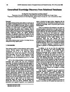
Table 1 Table name Australian Diabetes Iris Satellite
•
•
Nr of Objects 690 768 150 4435
Nr of Attributes 14 8 5 36
Training table 621 704 120 4435
generators from G cover the whole (or a large part of) domain. Compute “good” templates {T1, T2, …, Tm} covering {u1, u2, …, um}, respectively. The constructed templates determine a family of subtables. These sub-tables cover our domain. The maximal size of sub-tables can be set by user. Construct a minimal set of sub-tables covering a domain. One can use a greedy approximating algorithm for the minimal set cover presented in [22].
% � )�� ����� ������*����� � � ������� ��� � (� ���
Having the set of templates, one can decompose a domain into sub-tables. For any subtable we generate decision rules. Any new object is linked to sub-tables corresponding to templates covering this object. The object is classified using decision rules generated from these sub-tables. In Table 1 we present experimental results for some real data tables. In our experiments we used the discretization method (see e.g. [10]) to generate decision rules. We show the classification results of two methods of tests: • In the first method, called GLOBAL METHOD, we generate decision rules for the entire input training data and classify the new object using these decision rules. • In the second method, called LOCAL METHOD, we decompose the input data table into subtables and we classify the new object according to the schema described above. % % )�� ����� ������*����� �
��� �� ���� � � ��
�
����
Suppose we have a binary tree created in the process of decomposition as described in Section 4.1. For any new object we evaluate it starting from the root of the tree as follows: Let x be a new object, AT - a subtable containing all objects from the table A matching T and AT’ - a subtable containing all objects from A not matching T. 1. If x matches template T found for A then go to sub-tree related to AT else go to sub-tree related to AT’. 2. If x is at the leaf of the tree then go to 3 else repeat 1-2 substituting AT, AT’ for A, respectively. 3. Apply decision rules calculated [18] for subtable attached to the leaf to classify x.
Testing table 69 64 30 2000
GLOBAL METHOD 79,71% 67,85% 95,66% 81,8%
LOCAL METHOD 83,67% 70% 97,33% 83,6%
Presented above algorithm uses the binary decision tree, however it should not be misled with C4.5, ID3 and other algorithms using decision trees. The difference is that the above algorithm splits the object domain (universe) into sub-domains and for a new case we search for the most similar (from the point of view of the templates) sub-domain. Then rough set methods, C4.5, etc., may be used for the classification of this new case relatively to the matched sub-domain. In computer experiments we used generalised templates and attribute weight algorithm to create a binary decomposition tree. For Satellite Image data we obtained a tree of depth 3. Sub-domains of the training table of size from 200 to 1000 objects have been found during the tree construction. By evaluating the testing table using the constructed tree we have obtained at leaves testing sub-domains of size from 100 to 500 objects. Applying the decision rules [18] corresponding to the sub-domains we have obtained the overall quality of classification 82,6%. This is due to the fact that that there are leaves containing exceptions i.e. objects that do not match any (or very few) found template. Such leaves are in some sense chaotic and have worse quality of classification (about 70-80%) that decrease the overall score. However in many leaves of the tree the local quality of classification was much higher (about 90%). That means that using templates we found some good, uniform sub-domains with strong, reliable rules. ��� ��� � ��� ����� ���� ���� �������� �����
After the decomposition we obtain a set of reduced tables (agents [15]) which are able to produce a set of (local) decision rules. To obtain these rules we use a rough-set methods described in [18]. The main tool for calculating the rules for given information system (a decision table) is the notion of reduct. We are interested in short reducts, because these reducts give the best decision rules. However, the problem of minimal reduct finding is NP-hard. To find a set of possibly short reducts in a reasonable time, each agent uses a hybrid method with order-based genetic algorithm described in [24] and [25] with some improvements reducing a computational time. The main idea of this method is based on the following algorithm of reduct finding: take the set of all attributes, remove one of them and check whether it is still a superreduct (i.e. a reduct or its superset); if not - insert this
attribute back; else - try to remove the next attribute. This algorithm can generate any of the reducts; the result depends on the order of removing attributes. Our order-based genetic algorithm (see: [3], [2], [4]) is used to find the optimal order - i.e. an order generating possibly short reduct. The most time-consuming operation is determining whether a subset of attributes is a superreduct. Suppose we have a subset s. The algorithm of checking whether s is a reduct (or superreduct) works in the following steps: �?�� Observe, that if there exists a reduct r⊆s, then s is a superreduct. So, if we find such an r among the reducts found so far, the answer is YES. �?�� We can store all subreducts found so far in a fast to search, treelike structure. If we find our subset s in this structure, the answer is NO. '?�� If both of pervious steps fail, we are looking in our data for a pair of objects with equal values on attributes from s (see step d), but with the different decisions. If we find such a pair, answer is NO and we can add s to the tree of subreducts. If there is no such a pair, the answer is YES and we can add s to the list of (super)reducts, removing all its supersets. � To find a pair of objects described in c) one can insert all objects from the table into a binary tree - this is equivalent to sorting the data by the attribute values on s. � If such a pair is found, one can reorder objects and bring the pair to beginning. This can save up to 25% of computation time. It means, that if a pair of objects is a “counterexample” for one reduct, the same pair may be a “counterexample” for another. After each step of the genetic algorithm, the subsets collected in step c) are the reducts (not superreducts, see [24]). These reducts tend to be short, because the genetic algorithm seeks for the shortest ones. Our new method of reducts generation was tested on several data tables of different size. The results of experiments including computation time are presented below; the results are compared with the method described in [24]. Table size Comp. Time Comp. time, [s] old method [s] [obj×attr] 269 2,310 4,495×37 61 approx. 40,000 30,000×10 17.8 21.7 471×33 513 213 225×490 3 2,592 15,534×16 The experiment was performed on PC Pentium 100. Parameters of genetic algorithm: 10 generations, 10 individuals in population. The first two examples are well known “Satellite images” and “Shuttle” (reduced to 30,000 objects) tables. The algorithm produced about 80 short reducts for
each table, except the last one (where exists only one reduct). These results suggests, that our new method may be used to produce a set of short reducts in a reasonable time even for a table with thousands of objects. The algorithm has the average time complexity of (m2×N log N) where m - number of attributes, N - number of objects (the old version had the complexity of m2×N2). All the improvements described above work well for large tables with relatively small number of attributes this is the reason of poor results for 225×490 table. �� !���� � ���
We have presented some efficient methods for templates generation and a general scheme for approximate description of decision classes based on the notion of a template. An interesting aspect of our approach is that on the one hand searching methods are oriented towards uncertainty reduction in constructed descriptions of decision classes but on the other hand uncertainty in temporary synthesised descriptions of decision classes is the main "driving force" for the searching methods. The results of computer experiments are showing that the presented methods for template generation are promising even for large tables; however, much more additional work should be done on strategies for the construction of approximate decision class descriptions e.g. on the basis of the general mereological scheme [19]. The presented results create a step for further experiments and research on adaptive decision system synthesis.
��+� �����������9� ����� ��� � � �� � � ������� � ����� ���
�������������������� ��� ��������� ���� ��� ������� � ���� !���� ��" � #�� � �����$% References
[1] Thomas H. Cormen, Charles E. Leiserson, Ronald L. Rivest. The set-covering problem, pp.974-978. Introduction to Algorithms. The MIT Press, Cambridge, Massachusetts, London, England. [2] L. Davis (red.), 1991. Handbook of Genetic Algorithms. New York, Van Nostrand Reinhold. [3] D. E. Goldberg, 1989. GA in Search, Optimisation, and Machine Learning. AddisonWesley. [4] J.H. Holland, 1992. Adaptation in natural and artificial systems. The MIT Press, Cambridge. [5] J. R. Koza, 1992. Genetic Programming: On the Programming of Computers by Means of the Natural Selection. The MIT Press. [6] H. Mannila, H. Toivonen, A. I. Verkamo, 1994. Efficient algorithms for Discovering Association Rules. In: U. Fayyad and R. Uthurusamy (eds.): AAAI Workshop on Knowledge Discovery in Databases, pp. 181 - 192, Seattle, WA, July 1994.
[7] R. Michalski, G. Tecuci, 1994. Machine Learning. A Multistrategy Approach. Morgan Kaufmann, San Mateo, CA. [8] T. Mollestad, A. Skowron, 1996. A Rough Set Framework for Data Mining of Propositional Default Rules. Proc. ISMIS-96, pp. 448-457, Zakopane, Poland, June 1996.
A/B� �=� �=� 5�*���� �=� ���+����� �=� �*����� >7//C?=
������ �� � � � � �� �� � ��� ��������� �
� ���� �� � ��� ��� �� � ���
� =� �D"(./C9� (��
$������ ���2���� 3��5��##� ��� "���11�5��� (�'���4��#� ���� ��$�� 3�&2����5�� 22=� 7E/.76F� ��'����� ��&��*����2��&����,.6��7//C= [10] S. H. Nguyen, A. Skowron, 1995. Quantization of Real Value Attributes: Rough Set and Boolean Reasoning Approach. Proc. of the Second Annual Joint Conference on Information Sciences, pp. 34-37, Wrightsville Beach, NC, USA, September 28-October 1, 1995. [11] S. H. Nguyen, L. Polkowski, A. Skowron, P. Synak, J. Wróblewski, 1996. Searching of Approximate Description of Decision Classes. Proc. of The Fourth International Workshop on Rough Sets, Fuzzy Sets and Machine Discovery, RSFD’96, 153-161, Tokyo, November 6-8, 1996. [12] S. H. Nguyen, A. Skowron. Searching for Relational Pattern on Data. To appear in: Proc. of The First European Symposium on Principles of Data mining and Knowledge Discovery, Trondheim, Norway, June 25-27, 1997. [13] Z. Pawlak, 1991. Rough sets: Theoretical aspects of reasoning about data. Kluwer, Dortrecht. [14] G. Piatetsky-Shapiro, 1991. Discovery, Analysis and Presentation of Strong Rules. In: Piatetsky-Shapiro G. and Frawley W.J. (eds.): Knowledge Discovery in Databases, pp. 229 - 247, AAAI/MIT. [15] L. Polkowski, A. Skowron, 1996. Rough Mereological Approach to Knowledge-based Distributed AI. In: J.K. Lee, J. Liebowitz, Y. M. Chae (eds.): Critical Technology. Proc. of The Third World Congress on Expert Systems, pp. 774781, Seoul 1996, Cognisant Communication Corporation, New York. [16] L. Polkowski, A. Skowron, 1996. Rough mereology: A New Paradigm for Approximate Reasoning. To appear in: Journal of Approximate Reasoning
[17] J. R. Quinlan, 1993. C4.5: Programs for Machine Learning. Morgan Kaufmann, San Mateo, CA. [18] A. Skowron, 1995. Synthesis of Adaptive Decision Systems from Experimental Data. In: J. Komorowski, A. Aamodt (eds.): SCAI-95. Proc. Fifth Scandinavian Conference on Artificial Intelligence, pp.220-238, IOS Press, Amsterdam. [19] A. Skowron, L. Polkowski, 1995. Rough mereological foundations for analysis, synthesis, design and control in distributive system, Proc. Second Annual Joint Conference on Information Sciences, pp. 346-349, Sept. 28 - Oct. 1, 1995, Wrightsville Beach, NC. [20] A. Skowron, C. Rauszer, 1992. The discernibility matrices and functions in information systems. In: R. �G�+�H#�� (ed.): Intelligent Decision Support. Handbook of Applications and Advances of the Rough Sets Theory, pp.331 - 362, Kluwer, Dordrecht. [21] P. Smyth, R. M. Goodman, 1991. Rule introduction using Information Theory. In: Piatetsky-Shapiro G. and Frawley W.J. (eds.): Knowledge Discovery in Databases, pp. 159 - 176, AAAI/MIT. [22] H. Toivonen, M. Klemettinen, P. Ronkainen, K. Hatonen, H. Mannila, 1995. Pruning an Grouping Discovered Association Rules. In: Mlnet: Familiarisation Workshop on Statistics, Machine Learning and Knowledge Discovery in Databases, pp. 47 - 52, Heraklion, Crete, April 1995. [23] R. Uthurusamy, U. M. Fayyad, S. Spangler, 1991. Learning Useful Rules from Inconclusive Data. In: In: Piatetsky-Shapiro G. and Frawley W.J. (eds.): Knowledge Discovery in Databases, pp. 141 - 157, AAAI/MIT. [24] J. Wróblewski, 1995. Finding minimal reducts using genetic algorithms. Proc. of the Second Annual Join Conference on Information Sciences, pp.186-189, September 28-October 1, 1995, Wrightsville Beach, NC. [25] J. Wróblewski, 1996. Theoretical Foundations of Order-Based Genetic Algorithms. Fundamenta Informaticae, vol. 28 (3, 4), pp: 423-430. Kluwer, Dordrecht 1996. [26] W. Ziarko (ed.), 1994. Rough Sets, Fuzzy Sets and Knowledge Discovery, Workshops in Computing, Springer Verlag & British Computer Society.