Knowledge Transfer in Neural Networks: Knowledge-Based Cascade

Knowledge Transfer in Neural Networks: Knowledge-Based Cascade-Correlation

François Rivest

School of Computer Science McGill University, Montréal July 2002

A thesis submitted to the Faculty of Graduate Studies and Research in partial fulfillment of the requirements of the degree of Master in Science

© François Rivest, 2002

TABLE OF CONTENT

TABLE OF CONTENT ...........................................................................................I ABSTRACT .......................................................................................................... IV RÉSUMÉ................................................................................................................ V ACKNOWLEDGEMENT ....................................................................................VI CONTRIBUTION OF AUTHORS......................................................................VII STATEMENT OF ORIGINALITY ................................................................... VIII INTRODUCTION................................................................................................... 1 LITERATURE REVIEW........................................................................................ 3 Neural Networks ................................................................................................. 3 Multilayer Backpropagation Networks ........................................................... 3 Cascade-Correlation Networks ....................................................................... 8 Transfer of Knowledge in Neural Networks ..................................................... 12 Representational Transfer of Knowledge: Literal and Non-Literal Methods12 Functional Transfer of Knowledge: MTL..................................................... 18 Functional Transfer of Knowledge: Other Approaches ................................ 21 Symbolic to Neural Network Transfer .......................................................... 24 MANUSCRIPT 1 .................................................................................................. 26 Abstract ............................................................................................................. 27 1. Existing Knowledge and New Learning ....................................................... 28 2. Description of KBCC .................................................................................... 29 2.1 Overview ................................................................................................. 29 2.2 Networks and Units................................................................................. 29 2.3 Notation................................................................................................... 31 2.4 Output Phase ........................................................................................... 32 2.5 Input Phase .............................................................................................. 33 2.6 Connection Scheme in KBCC................................................................. 35 3. Applications of KBCC .................................................................................. 36 4. Finding and Using Relevant Knowledge ...................................................... 38

i

4.1 Translation............................................................................................... 38 4.2 Sizing....................................................................................................... 43 4.3 Rotation ................................................................................................... 51 5. Finding and Using Component Knowledge .................................................. 54 6. Summary of Learning Speed Ups ................................................................. 58 7. Generalization ............................................................................................... 59 8. Discussion ..................................................................................................... 60 8.1 Overview of Results ................................................................................ 60 8.2 A Note on Irrelevant Source Knowledge ................................................ 61 8.3 Relation to Previous Work ...................................................................... 61 8.4 Advantages of KBCC.............................................................................. 63 8.5 Future Work ............................................................................................ 66 Author Note....................................................................................................... 67 References ......................................................................................................... 67 CONNECTING TEXT.......................................................................................... 71 MANUSCRIPT 2 .................................................................................................. 72 Abstract ............................................................................................................. 73 I Existing Knowledge and New Learning ......................................................... 74 II Previous Work on Knowledge and Learning ................................................ 75 III Description of KBCC ................................................................................... 76 IV Demonstration of KBCC: Peterson-Barney Vowel Recognition................. 78 A. Experimental Setup .................................................................................. 79 B. Early Learning Comparison...................................................................... 80 C. Learning Time Comparison...................................................................... 82 D. Learning Quality....................................................................................... 83 E. Retention and 3rd Set Generalization ........................................................ 84 V Discussion ..................................................................................................... 84 B. Acknowledgments .................................................................................... 85 C. References ................................................................................................ 85 CONCLUSION ..................................................................................................... 88 KBCC and Other Approaches ........................................................................... 88

ii

Discussion ......................................................................................................... 89 Future Research................................................................................................. 90 APPENDIX I: KBCC MATHEMATICS ............................................................. 91 Cascade-Correlation Neural Networks.............................................................. 91 Notation......................................................................................................... 91 Activation ...................................................................................................... 93 Gradient......................................................................................................... 93 Hessian .......................................................................................................... 94 Knowledge-Based Cascade-Correlation Neural Networks ............................... 95 Notation......................................................................................................... 95 Activation ...................................................................................................... 97 Gradient......................................................................................................... 97 Hessian .......................................................................................................... 98 Knowledge-Based Cascade-Correlation Objective Functions .......................... 99 Notation......................................................................................................... 99 Objective Function ........................................................................................ 99 Gradient....................................................................................................... 100 REFERENCES.................................................................................................... 102

iii

ABSTRACT

Most neural network learning algorithms cannot use knowledge other than what is provided in the training data. Initialized using random weights, they cannot use prior knowledge such as knowledge stored in previously trained networks. This manuscript thesis addresses this problem. It contains a literature review of the relevant static and constructive neural network learning algorithms and of the recent research on transfer of knowledge across neural networks. Manuscript 1 describes a new algorithm, named knowledge-based cascade-correlation (KBCC), which extends the cascade-correlation learning algorithm to allow it to use prior knowledge. This prior knowledge can be provided as, but is not limited to, previously trained neural networks. The manuscript also contains a set of experiments that shows how KBCC is able to reduce its learning time by automatically selecting the appropriate prior knowledge to reuse. Manuscript 2 shows how KBCC speeds up learning on a realistic large problem of vowel recognition.

iv

RÉSUMÉ

La plupart des algorithmes d’apprentissage des réseaux de neurones ne peuvent utiliser des connaissances autres que celles contenues dans les données d’entraînement. Initialisés avec des poids aléatoires, ils ne peuvent utiliser de connaissances préexistantes telles que celles contenues dans d’autres réseaux entraînés antérieurement. Cette thèse traite de ce problème. Elle contient une revue de la littérature sur les algorithmes d’apprentissage des réseaux de neurones statiques et constructifs pertinents et des recherches récentes sur le transfert des connaissances entre les réseaux de neurones. Le premier manuscrit décrit un nouvel algorithme, nommé KBCC, qui améliore l’algorithme d’apprentissage cascade-correlation pour lui permettre d’utiliser des connaissances préexistantes. Ces connaissances préexistantes peuvent être fournies sous forme de réseaux de neurones entraînés. Le manuscrit contient aussi un ensemble d’expériences montrant que KBCC est capable de réduire son temps d’apprentissage en choisissant les connaissances préexistantes appropriées. Le second manuscrit montre comment KBCC accélère son apprentissage sur un problème réaliste d’envergure : la reconnaissance de voyelles.

v

ACKNOWLEDGEMENT

I am especially thankful to Professor Thomas R. Shultz. He gave me the opportunity to start doing real research when I was an undergraduate student, and for this, I can never thank him enough. He gave me the latitude to develop the ideas I had and that I believed in, while providing me with the necessary support and feedback to bring those ideas to life. I will always be thankful to the trust he showed in my research abilities. I am also thankful to Professor Doina Precup for her support and guidance through my graduate years at McGill. Her broad knowledge of my field allowed for insightful, constructive supervision. My work has also profited in one way or another from comments of fellow students David Buckingham, Reza Farivar, Jacques Katz, Sylvain Sirois, and JeanPhilippe Thivierge. Faculty members Yoshio Takane and Yuriko Oshima-Takane also contributed useful comments. The manuscripts profited from the comments of a few anonymous reviewers. I was fortunate to be supported by a grant from the Natural Sciences and Engineering Research Council of Canada and a grant from the Fonds de la Formation de Chercheurs et l’Aide à la Recherche to Thomas Shultz and by a grant from the Centre de Recherche Informatiqe de Montréal (CRIM) in collaboration with the Fonds de la Formation de Chercheurs et l’Aide à la Recherche to me. I am thankful to M. Pierre Dumouchel, VP at CRIM, for his useful support and supervision while I was there. Finally, I would like to thank my parents for their continuous belief in me and their encouragement in my academic aspirations. They were also always present in the last year when I needed a babysitter to be able to complete this work. I am also thankful to my wife Marie-Claude Bergeron for her continuous understanding and encouragement. I would like to dedicate my thesis to my daughter Mélodie and to my next child who should be born soon.

vi

CONTRIBUTION OF AUTHORS

Professor Thomas R. Shultz is the first author of the first paper and second author of the second paper. The original idea of recruiting whole, previously learned networks, in addition to single hidden units, was due to Professor Shultz. I developed the mathematics for KBCC, and implemented the algorithm, determining its details. In the first paper, I developed KBCC and conducted the experiments and data analysis. Design of the experiments was done collaboratively with Professor Shultz. In the second paper, professor Shultz contributed as my advisor, providing feedback and suggestions at all stages of my work.

vii

STATEMENT OF ORIGINALITY

Knowledge-based cascade-correlation (KBCC) is an original algorithm that I developed that extends the cascade-correlation algorithm (Fahlman & Lebiere, 1991). It is a new solution to the problem of transferring knowledge in neural networks that has fewer limitations than previous work and a higher level of automation (see conclusion).

viii

INTRODUCTION

Artificial neural networks reappeared in the 80s after being dismissed for a long period by the artificial intelligence community. It is only after they gained wide acceptance as AI tools and cognitive models that the problem of transfer of knowledge in neural networks really appeared as an important issue. The problem became more important in the early 90s, when a large number of applications based on neural networks were developed. Considering the huge amount of time required to train them, any speed improvement that could be gained when training a second version from a first one would be an asset. Similarly, considering the lengthy process of gathering data to train a successful network, any generalization that could be gained from re-using trained neural network knowledge to supplement the training set would also be an asset. Neural networks were also widely used as models of human cognitive abilities or development. The fact that these networks start from scratch while most human learning is based on prior experience (Pazzani, 1991, Wisniewski 1995) is a real-drawback. Moreover, simple re-training of a previously trained network on a new task showed catastrophic forgetting of the prior knowledge (McCloskey & Cohen, 1989), which is also inadmissible for any model of the human brain. The interest in the topic of knowledge transfer in neural networks reached its apogee in the mid 1990s. At NIPS 1995, there was a workshop organized by Baxter, Caruana, Mitchell, Pratt, Silver and Thrun on Learning to Learn: Knowledge Consolidation and Transfer in Inductive Systems.1 The following year, there was a special issue of Connection Science 8(2) on Transfer in Inductive System. Although a large amount of research took place, many of the problems raised by transfer of knowledge in neural systems remain unsolved. Despite some partial success, most applications and cognitive models are still built from scratch. Few solutions address the problem of changes in input encoding and output encoding from previously trained networks to new tasks. None address the unequal complexity of the various tasks a network may have to learn during its life. And many solutions are heavily restricted in 1

http://www-2.cs.cmu.edu/afs/cs.cmu.edu/user/caruana/pub/transfer.html

1

INTRODUCTION how prior knowledge is represented. Finally, much of the knowledge transfer must still be done by hand; for example, networks must usually be pre-selected to be reused. This thesis is an attempt to improve knowledge transfer in neural networks by presenting a novel algorithm called knowledge-based cascade-correlation (KBCC). KBCC is based on Fahlman and Lebiere’s (1991) cascade-correlation (CC) algorithm, which was shown to model many cognitive development phenomena (Shultz & Bale 2001, Buckingham & Shultz, 2000) as well as being able to deal with real applications (Yang & Honavar, 1998). KBCC inherits many of the useful properties of CC. Moreover, it has no restrictions in terms of input and output encoding of the prior knowledge. The only restriction on the form of prior knowledge in KBCC is that it be in the form of a function, and most knowledge can be represented in this way. KBCC automatically searches for relevant knowledge and uses only what is necessary. It also allows a new type of compositionality in knowledge transfer (see conclusion). This manuscript thesis begins with a literature review of the existing work on transfer of knowledge across neural networks. Then, the first manuscript, published in Connection Science, describes the KBCC algorithm in detail. This description is followed by a series of experiments showing how KBCC speeds up learning by using prior knowledge as well as a series of experiments demonstrating KBCC’s ability to choose the most appropriate sources and integrate them to learn a solution to the target task. This manuscript is followed by manuscript 2, published in the Proceedings of the 2002 International Joint Conference on Neural Networks, which documents the ability of KBCC to transfer knowledge on a large realistic problem. Finally, the conclusion compares KBCC to other approaches mentioned in the literature review, explains how KBCC addresses many important issues in knowledge transfer, and discusses further research.

2

LITERATURE REVIEW

Neural Networks Artificial Neural Networks encompass a wide range of architectures. This study of transfer of knowledge in neural networks is restricted to the so-called feedforward architecture. The justification for this choice is that, so far, most of the literature on transfer of knowledge in neural networks is on this architecture. Nevertheless, some transfer methods could be ported easily to other architectures, and some cases will be mentioned. Two types of feedforward networks have been studied for transfer of knowledge: layered feedforward networks, usually trained using the backpropagation algorithm, and cascaded feedforward networks, most often built and trained using the cascade-correlation algorithm. The former is probably the most common type of neural network. The latter is the basis of KBCC, a new algorithm I devised for the transfer of knowledge. KBCC is described in detail in manuscript 1 and improved in manuscript 2. Multilayer Backpropagation Networks Often called backpropagation networks, this class of networks can be more precisely described as multilayer feedforward neural networks trained using backpropagation of the error signal. This section first describes the architecture of this type of network, then its general training algorithm, and, finally, some of its known properties. Multilayer feedforward networks are made of two parts: layers of nodes, and sets of weights, as shown in Figure 1. Layers are collections of neurons. In this type of architecture, each layer feeds the next one through a set of weighted connections. Usually, every unit of a layer feeds every unit of the next layer. But a unit cannot feed any unit other than those on the next layer. If a unit was feeding a unit on a layer ahead that is not the next one, this would be a cross-connection. If a unit was feeding a unit on the same layer or on a previous layer, this would be a recurrent connection. The multilayered feedforward architecture discussed here contains neither cross-connections nor recurrent connections. 3

LITERATURE REVIEW

Figure 1: General multilayer feedforward neural network topology.

Usually, each layer is fed by the previous layer and by a bias unit, a constant giving the basic activity (see Table 1). For simplicity, this bias unit is often implemented as being part of the previous layer as shown in Figure 1.1 Input units are usually linear functions, i.e. their activation is given by the input pattern. For each non-input unit, its input is given by the weighted sum of the previous layer activations times the weight vector connecting the previous layer to the unit. This weighted sum is then passed through the unit’s activation function to obtain its output, or activation level, that will be an input for the next layer. The output layer activations corresponding to an input pattern are the associated output pattern of the network. Activation functions can have many forms. In the original work on perceptrons (McCulloch & Pitts, 1943, Rosenblatt, 1962), which generally had no hidden layers, the 0 if activation function was a simple threshold function of the form f ( x ) =  1 if

x < 0 . x ≥ 0

But Minsky and Papert (1969) showed that perceptrons could only solve linearly separable problems. Two sets of points are linearly separable if and only if there exist a hyperplane such that all points of the first set are on one side of it and all points of the other set are on the other side of it. Moreover, this function has the disadvantage of not 1

Note that it is equivalent to have all but the input layer fed by a single bias unit.

4

LITERATURE REVIEW being differentiable everywhere, and, hence, does not work with gradient descent optimization algorithms. The threshold function was therefore replaced by the sigmoid f (x ) =

1 and the hyperbolic tangent f ( x ) = tanh(x) functions2. These functions are −αx 1+ e

sometimes called soft threshold functions because they are a good differentiable approximation of the threshold function, as shown in Table 1. This led to a more general architecture with multiple layers, first invented by Bryson and Ho (1969), and popularized by Rumelhart et al. (1986) and the PDP Group in the mid-1980s. Many other functions were also studied, such as the ramp (continuous piece-wise linear), the augmented ratio of squares and the Gaussian. This last one is most often used in a slightly different architecture called radial basis networks, or networks of radial basis functions. Table 1 lists these functions with their mathematical definition and their graph. Note that all the functions mentioned above can be adjusted to match the desired output range using an affine transform of the form af ( x ) + b . Table 1: Most common activation functions with their definition and their graph.3

Function Name

Function Definition

Bias

1

Linear

2

Function Graph

f (x ) = x

In the sigmoid function, the α parameter is the so-called temperature parameter, usually set to 1 in this

architecture 3

This list is based in part from Eberhart, Simpson and Dobbins (1996).

5

LITERATURE REVIEW Threshold, step, or heaviside

0 if f (x ) =  1 if

x < θ x ≥ θ

Ramp or continuous

x < α

piece-wise linear

0 if  f ( x ) =  x if 1 if 

Sigmoid or logistic

f (x ) =

Hyperbolic tangent

f ( x ) = tanh (x )

Gaussian

α ≤ x < β x ≥ β

1 1 + e −αx

f (x ) = e

−

( x − µ )2 2σ 2

6

LITERATURE REVIEW Augmented ratio of squares

 x2  f ( x ) = 1 + x 2 0

if

x ≥ 0

otherwise

Training a multilayer feedforward neural network can be viewed as a straightforward optimization problem, where the weights are the parameters to optimize, and the sum squared error of the network on the training set is the objective function. Most of the time, a simple gradient descent approach, requiring the derivative of the objective function with respect to the weights, is used. Let N W : ℜ IN v ℜ OUT be the network function with weights W , where IN is the number of inputs and OUT the number   of outputs. Let {i p } ⊂ ℜ IN be the set of input patterns and {t p } ⊂ ℜ OUT be the   corresponding set of target patterns. If {o p = N W (i p )}⊂ ℜ OUT is the set of corresponding output patterns produced by the network, then the objective function is given by:   2 E = ∑ tp − op (1) p

  where v is the standard Euclidian norm of v . The update rule for the weights using gradient descent is then W(t +1) = W(t ) + ∆W(t ) , where W(t ) are the weights at time t,

∆W(t ) = −η

∂E ∂E , and is the partial derivative of E with respect to the weights W. ∂W (t ) ∂W (t )

This is usually called the backpropagation algorithm (BP). It is also current practice to add a momentum term updating the weights with ∆W(t ) = −η

∂E + α∆W(t −1) . Assuming ∂W (t )

a ball in weight space at position W on the error surface E, the gradient gives the direction and speed with which the ball should roll down from that position, while the momentum is analog to its current speed and direction. The momentum term makes the ball roll in a direction that is in part due to the current form of the error surface and in part due to the ball’s current direction.

7

LITERATURE REVIEW The objective function can also be modified to constrain the weights. By adding the proper penalty term to the objective function, one can force the weights to be small (add W ) or as orthogonal as possible (Golden, 1996). The objective function can also be modified to obtain invariance with respect to translation of the input by adding a penalty term based on the value of the slope (Mitchell, 1997).Finally, the objective function can also be the minimization of the cross-entropy of the output patterns (Hinton, 1989). In that case, and under certain assumptions, the output units are the probability density function of the output values, and the resulting algorithm (that does not need target patterns) is an unsupervised learner generating an Independent Component Analysis (ICA) (Comon, 1994) of the inputs. ICA is similar to Principal Component Analysis (PCA) but on higher order statistics. Finally, the optimization is in no way limited to the gradient descent algorithm. For instance, Fahlman developed Quickprop, which uses an estimate of the second order derivative (Fahlman, 1988). One could also use the second order Levenberg-Marquardt algorithms, Shannon algorithms or general conjugate gradient approach (Golden, 1996). More distributed algorithms could also be used, like the particle swarm optimization algorithm (that requires first order derivative) or basic genetic algorithms (which do not require derivatives and whose objective functions are called fitness functions), just to name a few (Eberhart, Simpson & Dobbins, 1996). An important known result about sigmoid-based multilayer feedforward networks is that two layers (one hidden layer of sigmoidal units with an output layer of linear units) are sufficient to approximate any continuous function to any arbitrary precision (Cybenko 1989; Hornick et al. 1989). Moreover, three layers (two hidden layers of sigmoidal units with an output layer of linear units) are sufficient to approximate any function to any arbitrary precision (Cybenko 1988). Cascade-Correlation Networks Multilayer feedforward networks are said to be static, because their structure is fixed at design time. A different approach is to use a network with a more dynamic structure, beginning with only a minimal number of units and connections, and letting it build its structure all by itself. There are at least two techniques that have been developed

8

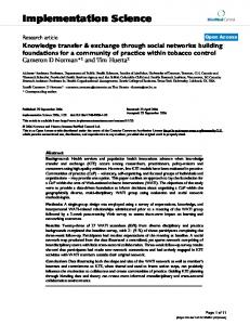
LITERATURE REVIEW to do this, and they appeared around the same time: splitting node networks by WynneJones (1992) and cascade-correlation networks (CC) by Fahlman and Lebiere (1990). This review is limited to the cascade-correlation architecture because it is the basis of the algorithm developed in the manuscripts. Many other constructive algorithms have been developed on the basis of cascaded networks and other similar architectures, some of which, like CC, are based on the work done originally by Gallant (1986). However, these other constructive approaches are more often designed to build classifiers rather than function approximators, which limits their use. Cascade-correlation networks differ from backpropagation networks in two ways. First, they do have cross-connections, and second, they construct their architecture automatically. In order to build the network architecture, CC alternates between two phases. In one phase, called the output phase, the weights feeding the output layer are trained similarly to backpropagation networks to reduce the error signal. In the other phase, the input phase, it is the weights feeding candidate units that might be installed in the network that are trained. A cascade-correlation network begins in output phase with only the bias unit, the input layer and the output layer. An example of a new network would be given in Figure 2, if only the input and output layers and their connections were considered. The weights are trained to minimize the sum of squared error as in backpropagation, usually using Quickprop. When the error stagnates, the network shifts to input phase.

9

LITERATURE REVIEW

Figure 2: General cascade network topology.

The first step of the input phase is to initialize a pool of candidate units. Those units (usually sigmoid or symmetric sigmoid) are fed by all but the output units. Each candidate is trained in parallel to maximize its covariance with the error patterns. If {ep = tp − o p }⊂ ℜOUT is the set of error patterns, and {vp }c ⊂ ℜ the set of corresponding activations for candidate c, then its objective function is given by: 4  ∑o Cov {v p }c , {e p ,o }  , where e p ,o is the oth element of vector e p .(2) Sc =  2 ∑ ep

(

)

p

Therefore, candidate units are biased toward being best at tracking the unresolved portion of the problem. When their score (the value of their objective function) stagnates, the best

4

A generalized mathematical definition of the network topology, derivative and objective function can be

found in Appendix I: KBCC Mathematics.

10

LITERATURE REVIEW unit is kept and a set of output weights between the new unit and the output layer is initialized with the proper sign (based on the sign of the covariance). The other candidates are discarded. Once a candidate is recruited and installed, the network shifts to output phase again. Whenever the network reaches the learning objective in output phase, the whole process stops. A final CC network has all the possible cross-connections and looks as shown in Figure 2. A particularity of this algorithm is that all the weights but the output ones are frozen. Hence, the same network could be used to learn another task without forgetting its knowledge stored in the hidden units (which are often considered to be feature detectors). Although CC in its original configuration has a lot of user defined parameters, in theory it should need fewer than backpropagation networks. The reason is that CC finds the right number of hidden nodes to reach the necessary computational power all by itself. Prechelt (1997) found that Rprop, a gradient descent algorithm using an adaptive learning rate and invented by Riedmiller & Braun (1986), was less sensitive to parameter variations than Quickprop. A debate still remains about whether hidden nodes should be cascaded or not, but Baluja and Fahlman (1994) have found that having both types of candidates (some that would be appended to the top most layer and some that would create a new layer) seems an excellent tradeoff, leading to compact networks of very few layers. Two important reviews of CC need to be mentioned. Prechelt (1997) has benchmarked different versions of CC on 42 different problems from the PROBEN1 database. Few general results were found. One general finding was that CC was superior for classification problems to an error minimization version of itself, which was superior on regression problems. Also, Waugh (1995) studied CC for function approximation, benchmarking CC, special connection schemes in CC, connections pruning in CC, and other extensions of CC. He found few positive improvements to CC, especially on phase stopping criteria and connections pruning. The literature contains more than a hundred papers on CC or variations of it. Finally, many of the variations discussed on BP learning can also be applied to CC. The type of candidate units can be as diverse as for BP, a penalty term can be added

11

LITERATURE REVIEW to the objective functions to favor certain properties, and the optimization algorithm is in no way restricted to Quickprop. There also exists a recurrent version of CC (Fahlman, 1991). Transfer of Knowledge in Neural Networks There are different types of transfer of knowledge in neural networks. The most important distinction is representational versus functional transfer (Pratt & Jennings 1996, Silver 2000). In representational transfer, it is the representation of the knowledge that is transferred either directly or indirectly. Direct methods are either literal or not. For example, a trained network can be copied, with (non-literal) or without (literal) minor changes to its weights and structures. It could also be transformed into an intermediate representation between its original and final representation (indirect method). On the other hand, in functional transfer, the representation is not directly involved. In this type of transfer, the knowledge is used to bias the training instead of the initial state of the network (Silver 2000)5. The learning may be biased by extra patterns, in one way or another, or the indirect use of previous learning experience. This section will deal with both types of transfer. First, there is a review of the work on representational transfer, from direct literal transfer to non-literal methods. Then, there is a review of the work on functional transfer of knowledge. Finally, research on the transfer of symbolic knowledge into neural networks is reviewed followed by a brief summary of other related work. The new algorithm developed in this thesis, called Knowledge-based Cascade-correlation, will not be covered here, because it is described in detail in manuscript 1. KBCC transfers the knowledge representation, without limiting that knowledge to any specific representation. It will be compared with the other methods presented here in the conclusion. Representational Transfer of Knowledge: Literal and Non-Literal Methods The simplest way to transfer knowledge from a trained network to a new network learning a task is to literally copy the trained network and train it on the new task as

5

Pratt and Jennings (1996) have a slightly different definition of representational and functional transfer.

Although both definitions are not totally incompatible, I found Silver’s (2000) definition more appropriate.

12

LITERATURE REVIEW shown in Figure 3. Although this may sometimes accelerate the learning, it may also slow it down (Pratt 1993a) and reduce the target network accuracy (Martin, 1988, mentioned in Pratt 1993b).Moreover, the re-trained network often loses its prior knowledge, a problem called catastrophic forgetting (McCloskey & Cohen, 1989). Forcing the hidden layer to be as orthogonal (i.e., that weight vectors feeding hidden units are orthogonal) and as distributed as possible seems to help, but it does not always work (French, 1992, 1994).

Figure 3: Literal transfer of knowledge.

Cascade-correlation is one of the first successful examples of literal transfer. Because all but its output weights are frozen once trained, only the output weights change when learning a second task. Hence, even if some new hidden units are added to its structure, the network can very rapidly recover its prior knowledge by re-adjusting the output weights properly. This is an example of transfer through sequential learning as shown in Figure 4.

13

LITERATURE REVIEW

Figure 4: Literal transfer of knowledge using sequential learning on a CC network.

A similar approach was also used by Parekh and Honavar (1998). Using the knowledge-based artificial neural network (KBANN6) algorithm (Towell and Shavlik, 1994) to transform symbolic knowledge into a neural network, they used the inputs of the current task as well as the outputs of the knowledge-based network to generate the inputs of a constructive algorithm. Note that this technique is not limited to symbolic knowledge. Any network could be copied and used to generate extra inputs for a new network to be trained. It is also not limited to constructive algorithms, it suffices that the new network contains as many inputs as the target task does plus the number of outputs of the prior knowledge as shown in Figure 5.

6

KBANN is discussed in the section on symbolic to neural network transfer.

14

LITERATURE REVIEW

Figure 5: Literal transfer of knowledge by using network outputs as extra inputs.

Another approach close to literal copying of a backpropagation network also appears to accelerate the learning of complex tasks. Instead of training a large network on some multi-output task, the task is first decomposed into subtasks corresponding to groups of different outputs. A small network is trained for each of these subtasks. The networks are then integrated into a larger network, as shown in Figure 6. Once that knowledge is transferred, the large network may be supplemented with some extra nodes, which are trained on the full task. The whole network may then be refined through full training. This approach, often called task decomposition, was used first used successfully by Waibel (1989) and then re-evaluated by Pratt (Pratt, Mostow & Kamm, 1991).

15

LITERATURE REVIEW

Figure 6: Transfer of knowledge by gluing trained sub-networks together.

A similar idea proposed by Hinton7 was to copy the trained networks to initialize a mixture of experts (ME) system (Jacobs, Jordan, Nowlan & Hinton, 1991). In this model, a number of networks are trained in parallel, each on a subset of the training patterns. At the output of the networks, there is a gating network that decides which network output to use for a specific input pattern. This leads networks to specialize on the subset of patterns they are best at mapping. This model is shown in Figure 7.

7

Personal discussion at McGill in February 2002.

16

LITERATURE REVIEW

Figure 7: Literal transfer of knowledge by using networks in a mixture of experts.

When prior knowledge is literally copied to a new task, some of the hyperplanes8 generated by the first layer of weights can be a bad fit for the new task and hence, may negatively affect the learning (when compared with a randomly initialized network) (Pratt, 1993a, 1993b). In order to solve this issue, Pratt (1993a, 1993b) devised a new algorithm called discriminality based transfer (DBT). The idea is to measure the discriminality of each hyperplane (unit in the first hidden layer). If a hyperplane is useful for the new task, its weights are scaled up to high values to keep it in place during learning. If a hyperplane is bad, its weights are reduced or even re-initialized to random values, assuming that a random hyperplane is more likely to become useful than a known bad hyperplane. Once this weight adjustment is accomplished, the network is trained using standard backpropagation.

8

A sigmoidal unit can be viewed at the extreme as a threshold function where the weighted sum at the

input determines a hyperplane. On one side of the hyperplane, the threshold unit is ON, on the other side, it is OFF.

17

LITERATURE REVIEW In Pratt’s work, the discriminality of a hyperplane is given by the mutual information measure, as in the construction of some decision trees. Discriminality is used to decide whether or not an existing hyperplane should be kept or changed. The mutual information is given by:

MI =

1 C  1 1 C  ∑∑ xi , j log xi , j − ∑ xi log xi − ∑ x j log x j + N log N  ,(3)  N  i = 0 j =1 i =0 j =1 

where N is the number of patterns, C the number of classes, j indexes over all classes, i indexes over the two sides of the hyperplane and x is the number of patterns in a given class (xj), or on a given side of the hyperplane (xi), or both (xi,j) (from Mingers 1989 as referenced by Pratt 1993b). Figure 8 and Figure 9 show examples, on a bi-dimensional input space, of two hyperplanes, one with a poor and one with a good discriminality, respectively.

Figure 8: Hyperplane with

Figure 9: Hyperplane with

poor discriminability.

good discriminability.

Pratt’s (1993a, 1993b) results suggest that this method has all the advantages of literal transfer without the drawbacks. She also surveyed a few other techniques related to weight adjustment in knowledge transfer, but they seemed to have less success. She also surveyed other knowledge transfer techniques (Pratt & Jennings 1996), some of which were not included in this thesis. Functional Transfer of Knowledge: MTL A different approach is to use only the network functionality rather than its implementation. In order to do that, Silver (2000) developed a technique based on results

18

LITERATURE REVIEW for multi-task learning by Baxter (1996) and Caruana (1995). The key idea is that when learning multiple tasks at the same time, the first set of weights of a two-layer neural network will build up a common representation useful to as many of the tasks as possible. In psychological terms, knowing about several problems related to the same concept gives a better grasp of that concept. Baxter’s (1996) work was mainly theoretical. He considered a multiple output network with each output corresponding to a different task and with at least a common hidden layer leading to all outputs. He showed that increasing the number of tasks reduced the necessary number of training patterns. More precisely, he showed that if O(a ) is the minimum number of patterns necessary to learn a single task, and if O(a + b ) is the minimum number of patterns to learn several tasks independently, then the network learning the tasks simultaneously requires only O(a + b n ) patterns, where n is the number of tasks. Caruana’s (1995) work was more empirical, but he provided a few reasons why learning multiple related tasks should be better than single task learning. The most important one is the fact that the hidden layer has pressure from all tasks, and hence, should find a better hidden representation. His empirical results showed that multi-task learning networks (MTL) generalized better than single-task learning networks (STL). Silver (Silver & Mercer, 1998; Silver, 2000) used MTL in conjunction with pseudo-rehearsing to transfer prior knowledge in new learning. He called this technique the task rehearsal method (TRM). Given a number of sources of knowledge for a total of Sn outputs and a target task of Tn outputs, let the new network to train have Tn + Sn outputs, one for each task output, as shown in Figure 10. The input patterns are first processed through the source networks. Then, the resulting output patterns are concatenated with the target patterns to generate the training set of the new network. This process of passing new input patterns through old networks to generate target patterns is called pseudo-rehearsal, where normal rehearsal would imply using the original patterns only. The network thus ends up relearning all the tasks that were part of the source knowledge at the same time as the new task, while generating at the hidden layer, a set of features that are likely to be useful for more tasks (a common representation) than if the network was trained only on the new task. 19

LITERATURE REVIEW

Figure 10: Functional transfer of knowledge through multi-task learning.

Silver (2000) has also shown that this procedure could be used on impoverished training sets, i.e., sets that contain too few patterns for proper learning. By generating extra input patterns and using them to generate extra outputs, the extra training that the hidden layers get from training the extra outputs (outputs matching the source networks outputs) may help the network discover the right internal representation for the target task. Silver (Silver & Mercer, 1996, Silver, 2000) also developed a variant of multitask learning (MTL) called ηMTL. The idea is to give each extra output a different learning rate from the target task. This is justified by the fact that the learning of those source tasks is not important in itself. What is important is the effect that learning them has on the internal representation of the network. The key is to evaluate, as training goes, how those source outputs relate to the target outputs. The more they relate, the closer their learning rate can be to the one of the target task. Unrelated tasks should be given very small learning rates, hence applying less pressure on the internal representation and reducing their potential interference. The learning rate η k for task k is given by:

20

LITERATURE REVIEW   1 SSE 1  , η k = η tanh 2 k ⋅  d k + ε RELMIN 

(4)

where, assuming a single target task k = 0, η is the target task learning rate, SSEk the sum squared error of the output k, dk the distance between the weight vector feeding output 0 and output k, ε > 0 and RELMIN the parameter controlling the rate of decay. Overall, knowledge transfer using pattern generation and ηMTL fills two goals, gaining efficiency (speed of learning) and effectiveness (accuracy). Silver’s work has achieved some success in both of these goals. Functional Transfer of Knowledge: Other Approaches Another approach is the idea of meta-learning developed by Naik and Mammone (1992). The general idea is to have a meta-network that learns how to learn as shown in Figure 11. Here, no direct prior knowledge is available, only traces of prior learning experiences are present. In the case of Naik and Mammone (1992), the meta-network receives as input the current weights of the network under training. Its output is a prediction of the final weights of the network under training. Predicted final weights and current weights are used to estimate an optimal weight direction and distance to move in that direction. This term is added to the standard weight update rule of backpropagation. Naik and Mammone (1992) showed that when the meta-network was trained on similar tasks, the algorithm converges faster than normal backpropagation and is less sensitive to initial weight values.

21

LITERATURE REVIEW

Figure 11: Functional transfer of knowledge through meta-learning.

Another dual network architecture is the idea of self-refreshing memory. The work of Ans and Rousset (2000) is a recent example of this older idea. Their specific network architecture is not covered here. Only the general scheme is described in this review. The model requires two similar networks, as shown in Figure 12. First, network 1 is trained on a task. Then, random input patterns are generated and processed through network 1 to generate outputs. These input-output pairs are then used to train network 2. Hence, network 2 is trained through pseudo-rehearsal of network 1. This process transfers the knowledge stored in network 1 to network 2. When network 1 needs to be trained on a new task, its training set is augmented by pseudo-rehearsed patterns from network 2. This way, network 1 learns the new task as well as its old knowledge, which it can refresh from the ‘storage’ represented by network 2. The main advantage of this technique is that it reduces catastrophic forgetting on sequential learning.

22

LITERATURE REVIEW

Figure 12: Functional transfer of knowledge through self-refreshing memory.

The last approach to functional transfer of knowledge covered here is called explanation based neural network (EBNN) and was develop by Thrun and Mitchell (1993). EBNN is a connectionist version of the symbolic explanation based learning algorithm (EBL). To maintain the analogy with EBL, it requires some domain theory and a standard training set for the new task. The domain theory must take the form of a differentiable function (as in KBCC, see manuscript 1). It could be a previously trained neural network or a KBANN (see next section) for example. Here, the prior knowledge will be used to explain the training data and help the target network to learn better.

23

LITERATURE REVIEW

  Given a set of input and target patterns ( {i p } and {t p }), EBNN first processes the  input patterns through the source network. This gives a set of output patterns ( {s p }). Then

it computes the derivative of the source knowledge output with respect to its input   ( {∂s p ∂i p }). These values are the explanation of each target pattern. The target network  is trained to learn the target values ( {t p }) as well as the source knowledge derivative   values ( {∂s p ∂i p }) using Tangent prop (Simard, Victorri, LeCun & Denker, 1992), as shown in Figure 13. Tangent prop is a variation of backpropagation that trains a neural network to fit not only its output to target values, but also its output derivative to target derivative values. The effect of learning derivatives is to learn existing invariances in the target function. The learning rate associated with the derivative of each pattern is determined by the distance between the target value and the source output   ( η p = 1 − s p − t p c ), i.e., by how much the source knowledge explains the data.

Figure 13: Functional transfer of knowledge through invariance learning.

Symbolic to Neural Network Transfer A slightly different problem is how to transfer symbolic or rule based knowledge into a new neural network. Pseudo-rehearsing methods partially answer this problem because, if the symbolic rules can be used as functions to generate target patterns, they

24

LITERATURE REVIEW can be used with MTL or a dual memory model. But this approach is based on relearning, which is not necessarily the way one may wish to reuse prior knowledge. Towell and Shavlik (1994) devised an algorithm specially made to integrate rules into a neural network named KBANN (knowledge-based artificial neural network). Their goal was to refine rule-based knowledge using neural networks as an intermediate step. They devised KBANN to transform rules into a network. The network was then trained on data for improvement and then rules were re-extracted from it using another algorithm. KBANN could be use to generate an initial network from which one could transfer knowledge to some other neural networks using the methods previously mentioned, or even KBCC (see manuscript 1). The work of Parekh and Honavar (1998) as well as Thrun and Mitchell (1993) are two examples where this technique could be applied.

25

MANUSCRIPT 1

Knowledge-based Cascade-correlation: Using Knowledge to Speed Learning

Thomas R. Shultz and François Rivest Laboratory for Natural and Simulated Cognition Department of Psychology and School of Computer Science McGill University

http://www.tandf.co.uk. Reprinted, with permission, from: Shultz, T.R. & Rivest F. (2001) Knowledge-based Cascade-correlation: Using Knowledge to Speed Learning. Connection Science 13(1):43-72.

26

MANUSCRIPT 1

Abstract Research with neural networks typically ignores the role of knowledge in learning by initializing the network with random connection weights. We examine a new extension of a well-known generative algorithm, cascade-correlation. Ordinary cascadecorrelation constructs its own network topology by recruiting new hidden units as needed to reduce network error. The extended algorithm, knowledge-based cascade-correlation (KBCC), recruits previously learned sub-networks as well as single hidden units. This paper describes KBCC and assesses its performance on a series of small, but clear problems involving discrimination between two classes. The target class is distributed as a simple geometric figure. Relevant source knowledge consists of various linear transformations of the target distribution. KBCC is observed to find, adapt, and use its relevant knowledge to significantly speed learning.

27

MANUSCRIPT 1

1. Existing Knowledge and New Learning Learning in neural networks is typically done "from scratch", without the influence of previous knowledge. However, it is clear that people make extensive use of their existing knowledge in learning (Heit 1994; Keil 1987; Murphy 1993; Nakamura 1985; Pazzani 1991; Wisniewski 1995). Use of knowledge is likely responsible for the ease and speed with which people are able to learn new material, although interesting interference of knowledge with learning can also occur. Neural networks fail to use knowledge in new learning because they begin learning from initially random connection weights. Here we examine a connectionist algorithm that uses its existing knowledge to learn new problems. This algorithm is an extension of cascade-correlation (CC), a generative learning algorithm that has proved to be useful in the simulation of cognitive development (Buckingham & Shultz, 1994; Mareschal & Shultz, 1999; Shultz 1998; Shultz, Buckingham, & Oshima-Takane, 1994; Shultz, Mareschal, & Schmidt, 1994; Sirois & Shultz, 1998). Ordinary CC creates a network topology by recruiting new hidden units into a feed-forward network as needed in order to reduce error (Fahlman & Lebiere, 1990). The extended algorithm, called knowledge-based cascade-correlation (KBCC), recruits whole sub-networks that it has already learned, in addition to the untrained hidden units recruited by CC (Shultz & Rivest, 2000a). The extended algorithm thus adapts old knowledge in the service of new learning. KBCC trains connection weights to the inputs of its existing sub-networks to determine whether their outputs correlate well with the network's error on the problem it is currently learning. Consistent with the conventional terminology of the literatures on analogy and transfer of learning, we refer to these existing sub-networks as source knowledge and to the current learning task as a target problem. These previously learned source networks compete with each other and with conventional untrained candidate hidden units to be recruited into the target network learning the current problem. As we discuss later, KBCC is similar in spirit to recent neural network research on transfer of knowledge, multitask learning, sequential learning, lifelong learning, input re-coding, knowledge insertion, and

28

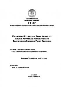
MANUSCRIPT 1 modularity, but it incorporates these ideas by learning, storing, and searching for knowledge within a generative network approach. We first describe the KBCC algorithm, show its learning speed performance on a number of learning problems that could potentially benefit from prior knowledge, and then discuss its advantages and limitations in the context of the current literature on knowledge and learning in neural networks. 2. Description of KBCC 2.1 Overview Because KBCC is an extension of CC, it uses many of CC's ideas and mathematics. As we describe KBCC, we note particular differences between the two algorithms. Both algorithms specify learning in feed-forward networks, adjust weights based on training examples presented in batch mode, and operate in two phases: output phase and input phase. In output phases, connection weights going into output units are adjusted in order to reduce error at the output units. In input phases, the input weights going into recruitment candidates are adjusted in order to maximize a modified correlation between activation of the candidate and error at the output units. Networks in both algorithms begin with only input and output units. During learning, networks alternate between input and output phases, respectively, depending on whether a new candidate is being recruited or not. We begin with the contrasting features of networks and units, and proceed to discuss the output phase, input phase, and connection scheme. 2.2 Networks and Units The major new idea in KBCC is to treat previously learned networks just like candidate hidden units, in that they are all candidates for recruitment into a target network. A sample KBCC network with two input units and a bias unit is pictured in Figure 1. This particular network has two hidden units, the first of which is a sub-network and the second of which is a single unit. Later hidden units are installed downstream of existing hidden units.

29

MANUSCRIPT 1

Output

Hidden 2

Hidden 1

Bias

Inputs

Figure 1. A KBCC network with two hidden units, the first of which is a previously learned sub-network and the second a single unit. The network is shown in the third output phase. Dashed lines represent trainable weights, and solid lines represent frozen weights. Thin lines represent single weights; thick lines represent vectors of weights entering and exiting the recruited sub-network, which may have multiple inputs and multiple outputs.

A single unit and a network both describe a differentiable function, which is what is required for learning in most feed-forward learning algorithms. In the case of a single unit, such as hidden unit 2 in Figure 1, this is a function of one variable, the net input to the unit. Net input to a unit i is the weighted sum of its input from other units, computed as: xi = ∑ wij a j

(1)

j

where i indexes the receiving unit, j indexes the sending units, a is the activation of each sending unit, and w is the connection weight between units j and i. The function for a single unit is often the centered logistic sigmoid function, in the range of -0.5 to 0.5: f ( x) =

1 − 0 .5 1 + e −x

(2)

30

MANUSCRIPT 1 where x is the net input to the unit. Other activation functions used in CC and KBCC are the asigmoid (logistic sigmoid) and Gaussian functions, both in the range 0.0 to 1.0. In the case of an existing sub-network, things are a bit more complicated because, unlike a single unit, there may be multiple inputs from each upstream unit and multiple outputs to each downstream unit, as illustrated by hidden unit 1 in Figure 1. For each such sub-network, the input weights and the output weights are each represented as a vector of vectors. Because the internal structure of a previously trained network is known, it can be differentiated in order to compute the slopes needed in weight adjustment, just as is commonly done with single hidden units. In KBCC, there is a list of current candidate networks, referred to as a parameter called CandidateNetworksList. We refer to the weights entering candidate hidden units and candidate networks as input-side weights. The input-side weights are trained during input phases as explained in section 2.5. 2.3 Notation Before presenting the algorithm in detail, it is helpful to describe the notation used in the various equations. wou ,o :

Weight between output ou of unit1 u and output unit o.

wou ,ic :

Weight between output ou of unit u and input ic of candidate c.

f o′, p :

Derivative of the activation function of output unit o for pattern p.

∇ ic f oc , p :

Partial derivative of candidate c output oc with respect to its input ic for

pattern p.

1

Vo , p :

Activation of output unit o for pattern p.

Voc , p :

Activation of output oc of candidate c for pattern p.

Vou , p :

Activation of output ou of unit u for pattern p.

To , p :

Target value of output o for pattern p.

We use unit to refer to any of the bias, input, or hidden units except when otherwise stated. Hidden units

include both single units and sub-networks.

31

MANUSCRIPT 1 2.4 Output Phase In the output phase, all weights entering the output units, called output weights, are trained in order to reduce error. As in CC networks, KBCC networks begin and end their learning career in output phase. The weights that fully connect the network at the start of training are initialized randomly using a uniform distribution with range [-WeightsRange, WeightsRange]. The default value is WeightsRange = 1.0. A bias unit, with an activation of 1.0, feeds all hidden and output units in the network. The output weights are trained using the quickprop algorithm (Fahlman 1988). The quickprop algorithm is significantly faster than standard back-propagation because it supplements the use of slopes with second-order information on curvature, which it estimates with the aid of slopes on the previous step. Quickprop has parameters for learning rate ε, maximum growth factor µ, and weight decay γ. The learning rate parameter controls the amount of linear gradient descent used in updating output weights. The maximum growth factor constrains the amount of weight change. The amount of decay times the current weight is added to the slope at start of each output phase epoch. 2 This keeps weights from growing too large. The default values for these three parameters are ε = 0.175/n, µ = 2.0, and γ = 0.0002, respectively, where n is the number of patterns. The function to minimize in the output phase is the sum-squared error over all outputs and all training patterns: F = ∑∑ (Vo , p − To , p )

2

o

(3)

p

The partial derivative of F with respect to the weight wou ,o is given by ∂F = 2∑ (Vo , p − To , p ) f o′, pVou , p ∂wou ,o p

(4)

The activation function for output units is generally the sigmoid function shown in Equation 2. Linear activation functions can also be used for output units. When the sigmoid function is used for output units, a small offset is added to its derivative to avoid getting stuck at the flat points when the derivative goes to 0 (Fahlman 1988). By default, this SigmoidOutputPrimeOffset = 0.1.

2

An epoch is a batch presentation of all of the traning patterns.

32

MANUSCRIPT 1 An output phase continues until any of following criteria is satisfied: 1. When a certain number of epochs pass without solution, there is a shift to the input phase. By default this number of epochs MaxOutputEpoch = 100. 2. When error reduction stagnates for few consecutive epochs, there is a shift to the input phase. Error is measured as in Equation 3, and must change by at least a particular proportion of its current value to avoid stagnation. By default, this proportion, called OutputChangeThreshold, is 0.01. The number of consecutive output phase epochs over which stagnation is measured is called OutputPatience and is 8 by default. 3. When all output activations are within some range of their target value, that is, when |Vo,p - To,p| ≤ ScoreThreshold for all o outputs and p patterns, victory is declared and learning ceases. By default, ScoreThreshold = 0.4, which is generally considered appropriate for units with sigmoid activation functions (Fahlman 1988). The ScoreThreshold for output units with linear activation functions would need to be set at the level of precision required in matching target output values. 2.5 Input Phase In the input phase, a new hidden unit is recruited into the network. This new unit is selected from a pool of candidates. The candidates receive input from all existing network units, except output units, and these input weights are trained by trying to maximize the correlation between activation on the candidate and network error. During this training, all other weights in the network are frozen. The candidate that gets recruited is the one that is best at tracking the network's current error. In KBCC, candidates include not only single units as in CC, but also networks acquired in past learning. N is the NumberCandidatesPerType, which is 4 by default. Weights entering N single-unit candidates are initialized randomly using a uniform distribution with range [-WeightsRange, WeightsRange] as in the output phase. Again, the default value is WeightsRange = 1.0. For each network in the CandidateNetworksList, input weights for N-1 instances are also initialized. Each input-side connection of these units is initialized using the same scheme as for the basic network weights, with one exception. The exception is that one instance of each stored network has its weight matrix initialized

33

MANUSCRIPT 1 with weights of 1.0 connecting corresponding inputs of target networks to source networks and weights of 0.0 elsewhere. This is to enable use of relevant exact knowledge without much additional training. We call this the directly connected version of the knowledge source. Activation functions of the single units are generally all sigmoid, asigmoid, or Gaussian, with sigmoid being the default. As in output phases, all of these input-side weights are trained with quickprop (with ε = 1.0/nh, 3 where n is the number of patterns and h is the number of units feeding the candidates, µ = 2.0, and γ = 0.0000). The function to maximize is the average covariance of the activation of each candidate (independently) with the error at each output, normalized by the sum-squared error. For candidate c, the function is given by

∑∑ ∑ (V

oc , p

Gc =

oc

o

)

− V oc (Eo , p − Eo )

p

# Oc ⋅# O ⋅ ∑∑ Eo2, p o

(5)

p

where E o is the mean error at output unit o, and V oc is the mean activation output oc of candidate c. The output error at pattern p is (Vo, p − To , p ) Eo , p =  (Vo, p − To , p ) f o′, p

if RawError = true otherwise

(6)

Gc is standardized by both the number of outputs for the candidate c (#Oc) and the number of outputs in the main network (#O). By default, RawError = false. 4 The partial derivative of Gc with respect to the weight wou ,ic between output ou of unit u and input ic of candidate c is given by

3

The 1/n (output phase) and 1/nh (input phase) fraction cannot be described as part of the objective

function of their respective phases as in standard back-propagation because ε is not used in the quadratic estimation of the curve in quickprop. It is a heuristic from Fahlman (1988) to set ε dynamically. 4

The variation of the error function Eo,p, which depends on RawError, comes from Fahlman's (1991) CC

code (ftp://ftp.cs.cmu.edu/afs/cs/project/connect/code/supported/cascor-v1.2.shar).

34

MANUSCRIPT 1

∂Gc = ∂wou ,ic

∑∑∑σ (E oc ,o

oc

o

o, p

)

− E o ∇ ic f oc , pVoc , p

p

# Oc ⋅# O ⋅ ∑∑ Eo2, p o

(7)

p

where σ oc ,o is the sign of the covariance between the output oc of candidate c and the activation of output unit o. An input phase continues until either of following criteria is met: 1. When a certain number of input phase epochs passes without solution, there is a shift to output phase. By default this MaxInputEpoch = 100. 2. When at least one correlation reaches a MinimalCorrelation (default value = 0.2) and correlation maximization stagnates for few consecutive input phase epochs, there is a shift to output phase. Correlation is measured as in Equation 5, and must change by at least a particular proportion of its current value to avoid stagnation. By default, this proportion, called InputChangeThreshold, is 0.03. The number of consecutive input phase epochs over which correlation stagnation is measured is called InputPatience and is 8 by default. When a criterion for shifting to output phase is reached, a set of weights is added from the outputs of the best candidate to each output of the network. All other candidate units are discarded, and the newly created weights are initialized with small random values (between 0.0 and 1.0), with the sign opposite to that in correlation. 2.6 Connection Scheme in KBCC Figure 2 shows the connection scheme for a sample KBCC network with two inputs, two outputs, one recruited network, and a recruited hidden unit. The recruited network, labeled H1 because it was the first recruited hidden unit, has two input units, two output units, and a single hidden unit, each labeled with a prime (') suffix. The main network and the recruited sub-network each have their own bias unit. Figure 2 reveals that the recruited sub-network is treated by the main network as a computationally encapsulated module, receiving input from the inputs and bias of the main network and sending output to later hidden units and the output units. Other than that, the main network has no interaction with the work of the sub-network.

35

MANUSCRIPT 1

Figure 2. Connection scheme for a sample KBCC network with two inputs, two outputs, one recruited network, and a recruited hidden unit.

3. Applications of KBCC To evaluate the behavior of KBCC, we applied it to learning in two different paradigms. One paradigm tests whether KBCC can find and use its relevant knowledge in the solution of a new problem and whether this relevant knowledge shortens the time it takes to learn the new problem. A second paradigm tests whether KBCC can find and combine knowledge of components to learn a new, more complex problem comprised of these components, and whether use of these knowledge components speeds learning. In each paradigm there are two phases, one in which source knowledge is acquired and a second in which this source knowledge might be recruited to learn a target problem. These experiments are conducted with toy problems with a well-defined structure so that we can clearly assess the behavior of the KBCC algorithm. In each problem, networks 36

MANUSCRIPT 1 learn to identify whether a given pattern falls inside a class that has a two-dimensional uniform distribution. The networks have two linear inputs and one sigmoid output. The two inputs describe two real-valued features; the output indicates whether this point is inside or outside a class of a particular distribution with a given shape, size, and position. The input space is a square centered at the origin with sides of length 2. Target outputs specify that the output should be 0.5 if the point described in the input is inside the particular class and -0.5 if the point is not in the class. In geometric terms, points inside the target class fall within a particular geometric figure; points outside of the target class fall outside of this figure. Networks are trained with a set of 225 patterns forming a 15 x 15 grid covering the whole input space including the boundary. For each experiment, there are 200 randomly determined test patterns uniformly distributed over the input space. These are used to test generalization, and are never used in training. We used this task to facilitate design and description of problems, variation in knowledge relevance, and identification of network solutions (by comparing output plots to target shapes). These problems, although small and easy to visualize, are representative of a wide range of classifier and pattern recognition problems. Knowledge relevance involved differences in the position and shape of the distribution of patterns that fell within the designated class (or figure). Degree of relevance was indexed by variation in the amounts of translation, rotation, and scaling. So-called irrelevant source knowledge involved learning a class whose distribution has a different geometric shape than the target class. We ran 20 KBCC networks in each condition of each experiment in order to assess the statistical reliability of results, with networks differing in initial output and input weights. Learning speed was measured by epochs to learn. Use of relevant knowledge was measured by identifying the source of knowledge that was recruited during input phases. In these experiments, networks learning a target task have zero, one, or two source networks to draw upon in different conditions. In each input phase of single source experiments, there are always eight candidates, four of them being previously learned networks and four of them being single units. In control conditions without knowledge (no source networks), all eight candidates are single units. These control networks are essentially CC networks. In conditions with two source networks in

37

MANUSCRIPT 1 memory, there are three candidates representing one source network, three candidates representing the other source network, and three single unit candidates. The reason for having multiple candidates for each unit and source network is to be able to provide a variety of initial input weights at the start of the input phase. This enables networks to try a variety of different mappings of the target task to existing knowledge. 4. Finding and Using Relevant Knowledge We did two kinds of experiments to assess the impact of source knowledge on learning a target task. In one kind of experiment, we varied the relevance of the single source of knowledge the network possessed to determine whether KBCC would learn faster if it had source knowledge that was more relevant. In a second kind of experiment, we gave networks two sources of knowledge, varying in relevance to a new target problem, to discover whether KBCC would opt to use more relevant source knowledge. To assess the generality of our results, we conducted both types of experiments with three different sets of linear transformations of the input space: translation, size changes, and rotation. In all of these experiments, KBCC networks acquired source knowledge by learning one or two problems and then learned another, target problem for which the impact of the previously acquired source knowledge could be assessed. We first consider problems of translation, then sizing, and finally rotation. 4.1 Translation5 In translation problems, degree of knowledge relevance was varied by changing the position of two-dimensional geometric figures. The target figure in the second (or target) phase of knowledge-guided learning was a rectangle with width of 0.4 and height of 1.6 centered at (-4/7, 0) in the input space. For translation problems, we first consider the effects of single-source knowledge on learning speed in the target phase and then the knowledge that is selected when two sources of knowledge are available.

5

A preliminary version of the translation results were presented in Shultz and Rivest (2000a).

38

MANUSCRIPT 1 4.1.1 Effects of Single-source Knowledge Relevance on Learning Speed In this experiment, networks had to learn a rectangle (named RectL) positioned a bit to the left of center in the input space, after having previously learned a rectangle, or two rectangles, or a circle at particular positions in the input space. The various experimental conditions are shown in Table I, in terms of the name of the condition, a description of the stimuli that had been previously learned in phase 1, and the relation of those stimuli to the target rectangle (RectL). Previous, phase-1 (or source) learning created the various knowledge conditions for the new learning of the target rectangle in the target phase. Conditions included exact knowledge (i.e., identical to the target), exact but overly complex knowledge, relevant knowledge that was either near to or far from the target, overly complex knowledge that was far from the target, and irrelevant knowledge. In a control condition, networks had no knowledge at all when beginning the target task, which is equivalent to ordinary CC. Table I: Single-source Knowledge Conditions for Translation Experiments

Name RectL 2RectLC RectC RectR 2RectCR Circle None

Description Rectangle centered at (-4/7, 0) 2 rectangles, centered at (-4/7, 0) and (0, 0) Rectangle centered at (0, 0) Rectangle centered at (4/7, 0) 2 rectangles, centered at (0, 0) and (4/7, 0) Circle centered at (0, 0) with radius 0.5 No knowledge

Relation to target Exact Exact/near, overly complex Near relevant Far relevant Near/far, overly complex Irrelevant None

A factorial ANOVA of the epochs required to reach victory yielded a main effect of knowledge condition, F(6, 133) = 33, p < .0001. Mean epochs to victory in each condition, with standard deviation bars and homogeneous subsets, based on the LSD post hoc comparison method, are shown in Figure 3. Means within a homogeneous subset are not significantly different from each other. Figure 3 reveals that exact knowledge, whether alone or embedded in an overly complex structure produced the fastest learning, followed by relevant knowledge, distant and overly complex knowledge and irrelevant knowledge, and finally the control condition without any knowledge.

39

MANUSCRIPT 1

2RectLC

Condition

RectL RectC RectR 2RectCR Circle None 0

200

400

600

800

Mean epochs to victory

Figure 3. Mean epochs to victory in the target phase of the translation experiment, with standard deviation bars and homogeneous subsets.

Some example output activation diagrams for one representative network from this simulation are shown in Figure 4. In these plots, white regions of the input space are classified as being inside the rectangle (network response > 0.1), black regions outside of the rectangle (network response < -0.1), and gray areas are uncertain, meaning that the network gives a borderline, unclassifiable response somewhere between -0.1 and 0.1. The 225 target training patterns, forming a 15 x 15 grid covering the whole input space, are shown as points in each plot. Figure 4a shows the source knowledge learned by this network in the exact but overly complex condition. The two white regions indicate the two rectangles constituting the target class for this condition. Such shapes are somewhat irregular, even if completely correct with respect to the training patterns, because they are produced by sampling the network on a fine grid of 220 x 220 input patterns.

40

MANUSCRIPT 1 a.

b.

c.

Figure 4. Output activation diagrams showing exact but overly complex source knowledge (a), the target network at the end of the first output phase (b), and the target solution at the end of the second output phase (c) after recruiting the source knowledge in (a).

Figure 4b shows this same KBCC system’s output at the end of the first output phase of target training. There are no white regions in this plot because the network has learned to classify most of the input patterns as being outside of the target class; the network is, on our definition, unsure of patterns within the first column of the input space. Because only 33 of the 225 training patterns fall within the target class, this is the best that the target network can do without any hidden units. Such behavior was common for the first output phase of learning a small rectangular target in every condition of every experiment reported in this paper.

41

MANUSCRIPT 1 Figure 4c shows this network’s final solution at the end of the second output phase of target training, after having recruited the source knowledge shown in Figure 4a. In this single-source experiment, exact but overly complex source knowledge was very effective in speeding up learning, as reported in Figure 3. Comparison of Figures 4a and 4c suggests that KBCC uses the recruited source network only when the input represented on the x-axis is less than about -3/14; otherwise it uses its direct input-tooutput weights. Examination of the output weights from the bias unit, the x-axis input unit, and the recruited hidden network confirmed that this is the case. These weights are such that the recruited hidden network can raise the weighted sum feeding the output unit above 0.0 only in the region of the target rectangle. Notice how closely the shape of the final solution in Figure 4c resembles that of the exactly correct portion of the source network in Figure 4a. Because one of the candidate source networks is initialized using direct input connections (i.e., weights that map input i to source network input i are set to 1.0 and all others to 0.0), KBCC always recruits that candidate source first in exact knowledge conditions. For 65% of these exact source networks, no further recruitment was necessary; for the remaining 35%, some additional recruitment was necessary to adjust to a few borderline patterns. A directly connected source candidate network was much less likely to be recruited in the close (25%) and far (0%) relevant conditions. 4.1.2 Selection of Relevant Knowledge from Two Sources In this experiment, networks first learned two tasks of varying relevance to the target task of learning RectL, the rectangle placed slightly to the left of the origin. The names of the various knowledge conditions, their relations to the target, and the mean times each network was recruited during input phases of target learning are shown in Table II. Descriptions of the figures designated by each condition name were provided in Table 1. The two recruitment means in each row were compared with a t-test for paired samples, except in the Exact vs. Relevant condition, where there was no variation in either variable. In every other case, the mean difference was significant at p < .001, df = 19. The pattern of differences shows that target networks preferred exact knowledge, even when it was embedded in overly complex knowledge. They also preferred simple

42

MANUSCRIPT 1 exact knowledge to overly complex knowledge that had exact knowledge embedded within it. Interestingly, a circle source was more often recruited than a source rectangle positioned at the right. Only two single-hidden-units were recruited by the 120 networks in this experiment. Table II: Dual-source Knowledge Conditions and Mean Networks Recruited in Translation Experiments

Name

Relation to target

RectL, RectR RectL, 2RectLC RectL, Circle RectR, 2RectLC RectR, Circle 2RectLC, Circle

Exact vs. Relevant Exact vs. Overly complex Exact vs. Irrelevant Relevant vs. Overly complex Relevant vs. Irrelevant Overly complex vs. Irrelevant

Mean networks recruited RectL RectR 2RectLC 1.0 0.0 n/a 0.95 n/a 0.15 1.05 n/a n/a n/a 0.15 1.25 n/a 1.25 n/a n/a n/a 1.45

Circle n/a n/a 0.0 n/a 2.55 0.15

The results of this dual-source experiment make sense given our analysis of the single-source experiment. Exact source knowledge is preferred over inexact source knowledge because it makes a nearly perfect match when accessed with direct connections. Overly complex exact source knowledge is less apt to be recruited than is simple exact source knowledge because it correlates less well with error in the case of directly connected sources. Perhaps the circle source knowledge is recruited over the far source rectangle because the circle is closer to the target rectangle even though it is the wrong shape. 4.2 Sizing In sizing problems, knowledge relevance was varied by changing the size of twodimensional geometric figures. The target figure in the second phase of knowledgeguided learning was a rectangle as were the figures in several of the knowledge conditions. Rectangles were always centered at (0, 0) in the input space and always had a height of 22/14. 4.2.1 Effects of Single-source Knowledge Relevance on Learning Speed In this experiment, several knowledge conditions varied the width of the firstlearned rectangle. Because scaling the width up and scaling the width down do not 43

MANUSCRIPT 1 produce the same results, we included conditions with either small or large target rectangles. The various conditions, which also included irrelevant knowledge in the form of a circle and no knowledge at all, are shown in Table III. Table III: Single-source Knowledge Conditions for Sizing Experiments

Name RectS RectM RectL Circle None

Description Rectangle of width 6/14 Rectangle of width 14/14 Rectangle of width 22/14 Center at (0, 0), radius 0.5 No knowledge

Relation to target RectL Far relevant Near relevant Exact Irrelevant None

Relation to target RectS Exact Near relevant Far relevant Irrelevant None

A factorial ANOVA of the epochs to victory when the small rectangle was the target yielded a main effect of knowledge condition, F(4, 95) = 103, p < .0001. The mean epochs to victory, with standard deviation bars and homogeneous subsets, based on the LSD post hoc comparison method, are shown in Figure 5. Relevant knowledge, regardless of distance from the target, produced faster learning than did irrelevant knowledge and no knowledge. This suggests that scaling down in size is not much affected by the amount of scaling required. The relatively few epochs required in phase 2 indicates that scaling down in size is relatively easy for these networks to learn.

Condition

RectL RectM RectS Circle None 0

100

200

300

400

500

600

Mean epochs to victory

Figure 5. Mean epochs to victory in the target phase of the small rectangle condition of the sizing experiment, with standard deviation bars and homogeneous subsets.

A factorial ANOVA of the epochs to victory when the large rectangle was the target also yielded a main effect of knowledge condition, F(4, 95) = 74, p < .0001, but with a somewhat different pattern of results. The mean epochs to victory, with standard 44

MANUSCRIPT 1 deviation bars and homogeneous subsets, based on the LSD post hoc comparison method, are shown in Figure 6. Exact knowledge yielded the fastest learning, followed in turn by near relevant knowledge, far relevant knowledge, and finally by no knowledge and irrelevant knowledge. This means that scaling up in size gets more difficult with the amount of scaling required. In this case, irrelevant knowledge did not speed up learning, as compared to the no-knowledge control. Examination of phase-1 source acquisition results confirmed that small rectangles were easier to learn than large rectangles, in terms of both hidden units recruited and epochs to learn.

Condition

RectL RectM RectS None Circle 0

200

400

600

800

1000

Mean epochs to victory

Figure 6. Mean epochs to victory in the target phase of the large rectangle condition of the sizing experiment, with standard deviation bars and homogeneous subsets.

When learning a small target rectangle, the percent of networks recruiting a directly connected source network decreased from 100% in the exact source knowledge condition to 80% in the near relevant source knowledge condition to 45% in the far relevant source knowledge condition. Figures 7 and 8 present output activation diagrams for networks learning a small target rectangle, recruiting either near relevant or far relevant directly connected source knowledge, respectively. Again, in both cases, there is a striking resemblance between the shape of the source knowledge and that of the final solution. As with translation experiments, the networks here learn to classify all patterns as being outside of the target class during the first output phase.

45

MANUSCRIPT 1 a.

b.

Figure 7. Output activation diagrams for a network learning a small rectangle, showing near relevant source knowledge (a) and the final target solution at the end of the second output phase (b) after recruiting the knowledge in a.

a.

b.

Figure 8. Output activation diagrams for a network learning a small rectangle, showing far relevant source knowledge (a) and the final target solution at the end of the second output phase (b) after recruiting the knowledge in a.

However, when learning a large target rectangle, networks do the opposite; that is, they learn to classify all patterns as being inside of the target class during the first output phase. This is because many more of the training patterns (121 of 225) fall within the target class when the target is a large rectangle. The percent of networks recruiting the directly connected source network when learning a large target rectangle was 100% in the exact and near source knowledge conditions and 75% in the far relevant source 46

MANUSCRIPT 1 knowledge condition. Figures 9 and 10 show output activation diagrams for networks learning a large target rectangle, with either near relevant or far relevant source knowledge, respectively. a.

b.

c.

d.

Figure 9. Output activation diagrams for a network learning a large rectangle, showing near relevant source knowledge (a) and target solutions at the end of the second (b), third (c), and fourth and final (d) output phases.

47

MANUSCRIPT 1 a.

b.

c.

d.

Figure 10. Output activation diagrams for a network learning a large rectangle, showing far relevant source knowledge (a) and target solutions at the end of the second (b), fifth (c), and sixth and final (d) output phases.

Any lingering error during target learning, whether scaling down to a small rectangle or scaling up to a large rectangle, involves patterns near the four corners of the target rectangle, such corners being regions of intersecting hyper-planes being learned by the network. When scaling down to learn a small target rectangle, network recruitment sharpens these corners, making target learning rather fast. In contrast, when scaling up to a large target rectangle, network recruitment smoothes these corners, thus prolonging target learning in order to re-sharpen the corners. When scaling up to a large rectangle, the amount of corner smoothing and eventual re-sharpening grows with the degree of scaling. Because no additional sharpening of corners is required when scaling down to a

48

MANUSCRIPT 1 small rectangle, learning speed is rather fast and does not vary with the degree of scaling required. Mean input connection weights for the critical x-axis input units learned in the sizing experiment while recruiting a directly connected source network are plotted in Figure 11. Because recruiting exact knowledge requires no rescaling of inputs, these connection weights are about 1, regardless of the size of the target rectangle. With a small target rectangle, these weights increase with the amount of scaling required; with a large target rectangle, these weights decrease with the amount of scaling required. Such trends make sense because when scaling down to a small target rectangle, the inputs to the small target would need to be scaled up with larger weights in order to effectively use the larger source network. In contrast, when scaling up to a large target rectangle, the inputs to the large target would need to be scaled down with smaller weights in order to effectively use the smaller source network. During these recruitments, connection weights for y-axis input units were always about 1 because rectangle height was constant, and all other connection weights were about 0 because they were unimportant.

Mean weight

3

2

Exact Close Far

1

0 Small

Large Target

Figure 11. Mean input connection weights for x-axis input units learned in the sizing experiment while recruiting a directly connected source network.

49

MANUSCRIPT 1 4.2.2 Selection of Relevant Knowledge from Two Sources In this experiment, networks first learned two tasks of varying relevance to the target task. The names of the various knowledge conditions, their relations to the target, and the mean times each network was recruited during input phases are shown in Table IV. The descriptions of the figures associated with each condition name were provided in Table III. The two means in each row were compared with a t-test for paired samples. Results are shown in the last two columns of Table IV. Exact knowledge was preferred over relevant or irrelevant knowledge. Relevant knowledge was preferred over irrelevant knowledge only when scaling down to a smaller rectangle. The large number of recruited networks in the relevant vs. irrelevant, scaling-up condition reflects the relative difficulty of learning in this condition. Again, the longer that learning continues the more recruitment is required. In this experiment, two of the 120 networks each recruited 1 single-hidden-unit, and two others recruited 2 single-hidden-units, for a total of 6. All six of these hidden units recruited were all in the scaling-up conditions of the experiment. Table IV: Dual-source Knowledge Conditions and Mean Networks Recruited for Sizing Experiments

Name

Target: RectS RectS, RectL RectS, Circle RectL, Circle Target: RectL RectL, RectS RectL, Circle RectS, Circle

Relation to target

Mean networks t(19) recruited RectS RectL Circle

p