222
IEEE TRANSACTIONS ON NEURAL NETWORKS, VOL. 13, NO. 1, JANUARY 2002
Neural Networks With Multidimensional Transfer Functions C. Tsitouras
Abstract—We present a new type of neural network (NN) where , the vector y the data for the input layer are the value associated to an initial value problem (IVP) with y ( ) = (y( )) and a steplength . Then the stages of a Runge–Kutta (RK) method with trainable coefficients are used as hidden layers for the integration of the IVP using as transfer function. We take as output two estimations y y ^ of IVP at the point + . Training the RK method at some test problems and counting the cost of the method under the coefficients used, we may achieve coefficients that help the method to perform better at a wider class of problems.
with and is strictly lower triangular. The procedure that advances the solution from to computes at each step two approximations to of orders and , respectively, given by
Index Terms—Initial value problem (IVP), orbits, oscillators, Runge–Kutta (RK), vector transfer function.
and
NOMENCLATURE
with
for RK
. From this embedded form (called ) we can obtain an estimate
of the local truncation error of the step-size control algorithm
order formula. So the
TOL
I. INTRODUCTION
E
XPLICIT Runge–Kutta (RK) pairs are widely used for the numerical solution of the initial value problem
where . These pairs are characterized by the extended Butcher tableau [2], [7]
(1)
is in common use, with TOL being the requested tolerance. The , but above formula is used even if TOL is exceeded by is simply the recomputed current step. See [28] for then more details on the implementation of these type of step size policies. Less experienced readers are refered to [14, p. 173], while [2], [7] are classical for the area of numerical analysis of ordinary differential equations. II. DERIVATION OF RK PAIRS The derivation of better RK pairs is of continued interest the last 30–40 years [6], [5], [17], [31], [20], [23], [24], [19]. The main framework for the construction of RK pairs is matching after we have Taylor series expansions of expanded various ’s. The final series has the form
Manuscript received November 3, 2000; revised June 4, 2001. The author is with the Department of Applied Mathematical and Physical Sciences, National Technical University of Athens, GR 15780 Athens, Greece (e-mail:
[email protected]). Publisher Item Identifier S 1045-9227(02)00359-4. 1045–9227/02$17.00 © 2002 IEEE
IEEE TRANSACTIONS ON NEURAL NETWORKS, VOL. 13, NO. 1, JANUARY 2002
In this expansion scalars pending explicitly on
etc.
are the th order conditions deand . e.g.,
’s
are elementary differentials of , e.g., , etc. See [2, pp. 170–171] for a list of order conditions and the coresponding elementary differentials. So in order to derive a third-order RK method we set and we have to satisfy four equations for the six coefficients (by default , restricts ). Once a third-order method is found, nothing can be said about the errors it may produce when applied to some problem since the magis unpredictable. Some better accuracy is nitude of expected if we reduce the norm of the principal truncation error
where , are the conditions for satisfying order . Values of for various orders are given in Table I. This technique is used widely for derivation of better RK of higher orders too [5], [21], [17], [20], [26]. The order conditions are solved using various simplifying assumptions considering different families of pairs. After we express all the coefficients of the family with respect to some free parameters we for these parameters. Although continue minimizing for a -order RK method seems the minimization of best choice for a general problem, a lot of speculation is raised ’s can be handled. Such for problems where it is believed that problems are Hamiltonians [3], orbits [25], periodic [29], [16], [19], Schrödinger [1] and many others. Unfortunately in most cases analytical consideration of test problems produces complicated algebra and enforces us to proceed with oversimplifications. In other cases we deal with some side properties such as symplectiness, [7, p. 312]. Tenths of symplectic RK methods were appeared last years and no one of them was even competitive to the conventional ones. An interesting alternative could be the consideration of RK type neural networks (NNs), where the various new families pairs are tested on some model problems to give good predictions for their coefficients. III. RK NEURAL NETWORK The literature combining numerical analysis and especially numerical IVP and NNs is limited. Lagaris et al. [13] presented a neural-network approach of solving IVP, but they do not give comparisons with the traditional multistep or RK methods. Multistep methods depending directly and linearly on a set of points give extremely accurate results. In [13] ten points are used and it seems theoretically difficult to compete multistep methods
223
TABLE I NUMBER OF ORDER CONDITIONS FOR VARIOUS ORDERS
with minimizations requiring repeated calls of and evaluations or even inversions of Jacobians. Recent literature has answered for the most of the claimed there drawbacks of discrete methods. For example RK can be combined with continuous [27] or highly differentiable solution [18]. Perhaps their technique is promising in parallel computers or stiff systems where nonlinear equations has to be solved anyway. Recently Wang and Lin [32] proposed the so called RK NNs. Their approach is from system identification point of view and they are interested in estimating the function by an NN. They used a classical RK method [12] of fourth order with constant stepsize because it is easier to prove some theoretical results. From practical consideration we might observe better results when using newer higher order methods with variable stepsize implementation. Perhaps some modification is needed for the learning algorithms reported there, since the simplification of dealing with scalar problems does not work for RK of orders exceeding 3 [14, p. 173]. In this paper we neither indent to solve IVP nor to verify the function . We are interested in deriving better RK pairs of a using stages. Thus we introduce a prescribed order feedforward NN consisted from hidden layers and each one contains neurons. INPUT:
and the function
First hidden layer: Second hidden layer: Third hidden layer:
th hidden layer: OUTPUT:
The corresponding drawing of the above NN is shown in Fig. 1. The NN we introduced is more general than a common multilayer NN since at each neuron acts a different component of the multidimensional function . This NN can be trained for and furnish a variety of inputs the proper coefficients achieving the desirable minimization of the value
224
Fig. 1.
IEEE TRANSACTIONS ON NEURAL NETWORKS, VOL. 13, NO. 1, JANUARY 2002
The neural system calculating R-K coefficients.
It is supposed that ’s belong to the same parametric type of functions and most of the times are identically the same. If we do not know the analytical solution of the IVP (to be avoided for model problems) we may estimate the true values of the sample by an accurate integration with higher order points method at very stringent tolerance. Let us illustrate now a paradigm for the derivation of the gradient directions that can be used to derive learning algorithms. we take . We can For the third-order RK method
easily derive a two parameter general family of coefficients depending on the values . So we have [2, p. 174]
IEEE TRANSACTIONS ON NEURAL NETWORKS, VOL. 13, NO. 1, JANUARY 2002
be determined dynamically. The tolerance TOL and the region where we want to test the RK pair determine the whole line of NN. The output of each NN is and in order to evaluate a new step based on (1). Then we may proceed to the next NN in line with inputs and of course the transfer function . The number of inputs is dynamically determined each time we backpropagate for another training and the value we get as final output is the efficiency of the pair which is to be optimized. It is worth to notice that there might be rejections of some NN is not less than TOL. The cost of evaluating from this line if these NN must be also considered in the final evaluation of the efficiency eff. So here we simply choose
and we need to evaluate only
with
The cost of the pair for the integration we made is not simply at grid points but it has to involve the the true global error needed. A measure of the eftotal number of -evaluations ficiency is presented in [22]
and similarly
If we expand
225
in power series of
, we get
where
TOL The smaller the eff the better the efficiency, so we indent to minimize eff for some test IVPs hoping for a better performance in a wider class of problems. and In the latter case the values of the form of the paradigm concerning third-order RK methods are difficult to evaluate because the various elementary the differentials are changing every time. Denoting by corresponding elementary differential of the -th input we calculate
and
Evaluating the elementary differentials at is supposed to be an easy task for a model problem. They are also evaluated in the once at the beginning of training only. Notice scalar case, but this is not true for systems of equations since and are matrices then. The technique we used is obligatory since the analytic evalis difficult, while the presented uation of algorithms are valid even for higher order methods. Then there are a little more parameters (e.g., for a fifth-order method there are only four parameters), and the calculations are straightforward following RK theory. A very interesting realization of the above algorithm may test the reliability of the error estimator combining many NNs in line, where the output of the first is input for the second just like we proceed with RK steps when integrating an IVP. In this case a small modification is required since the input data must
Since that depend on the RK method remain constant during the integration, we may admit some averaging value of the form
with
This means that we follow the direction of minimizing the principal truncation error coefficients of the RK formula hoping that will lead us to a better choice. In alternative we may evaluate
with
the average step size.
226
IEEE TRANSACTIONS ON NEURAL NETWORKS, VOL. 13, NO. 1, JANUARY 2002
IV. NUMERICAL RESULTS FOR PAIRS OF ORDERS 5(4) The initial idea of producing coefficients without satisfying any order condition was a total failure. Actually our technique has reason in existing families where most of the coefficients are expressed with respect to a small number of them served as free parameters. Here, we will try to produce more efficient RK5(4) pairs. Pairs of orders 5(4) are the most popular ones and can easily found in the literature. Matlab [15], has included the standard function ode45, which uses perhaps the most famous such pair DP5(4) due to Dormand and Prince [5]. For this pair we have but the last stage of each step may reused as the first stage in the next step (FSAL). So only six evaluations of the transfer function are wasted every step since the last layer of the some NN in line is placed again as first layer for the next NN. We name this property last layer as first (LLAF). In [17], we may find an algorithm where all the coefficients of a 5(4) pair may expressed explicitly based on the parameters and . Reproducing a learning algorithm here we have to evaluate the 20 truncation error values and differentiate them with the free parameters. A. Kepler Orbital Problem The problem has the form
a) . We recorded the 63 values while of eff and found that in average , reducing the cost for the new pair we have 33%. b) . We recorded again the 63 values of eff and found that in average while for the new pair we have , reducing the cost 35%. c) . We recorded again the 70 values of eff and found that in average while for the new pair we have , reducing the cost 34%. So the pair we derived optimizing a simple integration has some hidden property that helps it to perform much better than conventional pairs for every test in the family of two body (Kepler) problems. We can not obtain this hidden property with a . In [20] a new optimal RK pair simple minimization of of orders 6(5) was found with minimized truncation error, but when tested on Kepler problem it was 30% less efficient than older methods for some eccentricities, while there were eccentricities where it was almost 50% more efficient. Here the observed deviation from the mean value of efficiency is very small. Gaining in average 10–15% for methods of the same order is the usual improvement of RK pairs through the years passed [6], [5], [17]. Gaining here more than 30% is worth mention. B. Periodic Problems When dealing with periodic or oscillatory problems it is constructive to consider the test equation
where with the eccentricity of the orbit. The left superscript denotes the component of . It is known that the energy
remains constant since the problem is conservative. So we conover sidered as ge the maximum observed value of all the grid points. We applied the NN described above with inputs and TOL . Simulating NN with DP5(4) coefficients . Then we proceed training the NN we found for the new method which line obtaining finally means that it was almost 72% less expensive than DP5(4). The optimal efficiency was found for
The coefficients of the new pair NEW5(4)a can be derived applying the algorithm in [17], and are listed in Table II. We test the result with simulation for a wide class of regions, eccentricities, and tolerances. We include here three simulations.
The theoretical solution of this problem is
In many applications we are interested on the argument , i.e., of the solution which is the phase of the angle , [29], [19]. Monitoring this value through the integration we ensure that we remain in phase. So we considered as ge the maximum observed value of over all the grid points. We applied the NN described above with inputs and TOL . Simulating NN with DP5(4) coefficients . Then we proceed training the NN we found for the new method which line obtaining finally means that it was almost 800% less expensive than DP5(4). The optimal efficiency was found for
The coefficients of the new pair NEW5(4)b can be derived applying the algorithm in [17], and are listed in Table III. We test the result with simulation for a wide class of regions, frequencies, and tolerances. We include here three simulations. a) . We recorded the 70 values of eff and found
IEEE TRANSACTIONS ON NEURAL NETWORKS, VOL. 13, NO. 1, JANUARY 2002
227
TABLE II COEFFICIENTS OF NEW5(4)A (ACCURATE AT 16 DIGITS)
TABLE III COEFFICIENTS OF NEW5(4)B (ACCURATE AT 16 DIGITS)
that for the new pair we have in average while for DP5(4) we have , and this means that it is 245% more expensive. TOL b) . We recorded again the 70 values of eff and , found that in average for the new pair we have i.e., 275% while for DP5(4) we have more expensive. TOL c) . We recorded again the 70 values of eff and , found that in average for the new pair we have i.e., again while for DP5(4) we have about 275% more expensive. So we again derived a pair optimizing a simple integration of the test periodic problem. We did not get better results by using a more analytical approach [19]. Besides the NN technique may
expand to inhomogeneous problems where the analysis is very difficult, e.g., [30]
or even to nonlinear ones. V. CONCLUSION A new type of artificial NN design was proposed in this paper for the derivation of the coefficients of Runge-Kutta pairs for the numerical solution of initial value problems. The system described in this paper is more general than multilayer NN considered in the classic articles on approximation problems [4] and [8]–[11]. We also show an example of a system for which is not true that one hidden layer is sufficient to solve the problem.
228
IEEE TRANSACTIONS ON NEURAL NETWORKS, VOL. 13, NO. 1, JANUARY 2002
The main features of the new proposal are: 1) vector transfer functions; 2) dynamic changing of input data; 3) LLAF; 4) backpropagating in the direction of minimizing principal truncation error of the numerical scheme. A first interesting result is that we can produce better IVP solvers for various types of problems. This was achieved by training them in a test problem and optimizing their coefficients. ACKNOWLEDGMENT The author wishes to thank the anonymous referee for drawing Fig. 1. REFERENCES [1] G. Avdelas, T. E. Simos, and J. Vigo-Aguiar, “An embedded exponentially fitted Runge-Kutta method for the numerical solution of the Schrödinger equation and related periodic initial value problems,” Comput. Phys. Commun., vol. 131, pp. 52–67, 2000. [2] J. C. Butcher, The Numerical Analysis of Ordinary Differential Equations. New York: Wiley, 1987. [3] M. P. Calvo and J. M. Sanz-Serna, “High order symplectic Runge-KuttaNyström methods,” SIAM J. Sci. Comput., vol. 14, pp. 107–114, 1993. [4] G. Cybenko, “Approximation by superpositions of a sigmoid function,” Math. Contr. Signals, Syst., vol. 2, pp. 303–314, 1989. [5] J. R. Dormand and P. J. Prince, “A family of embedded Runge-Kutta formulae,” J. Comput. Appl. Math., vol. 6, pp. 19–26, 1980. [6] E. Fehlberg, “Low order classical runge-kutta formulas with stepsize control and their application to some heat-transfer problems,”, TR R-287, NASA, 1969. [7] E. Hairer, S. P. Nrsett, and G. Wanner, Solving Ordinary Differential Equations I, 2nd ed. Berlin, Germany: Springer-Verlag, 1993. [8] R. Hecht-Nielsen, “Counterpropagation networks,” in Proc. Int. Conf. Neural Networks. New York, 1987, pp. 19–32. , “Kolmogorov’s mapping neural network existence theorem,” in [9] Proc. Int. Conf. Neural Networks. New York, 1987, pp. 11–13. , Neurocomputing. Reading, MA: Addison-Wesley, 1990. [10] [11] K. Hornik, “Approximation capabilities of multilayer feedforward networks,” Neural Networks, vol. 4, pp. 251–257, 1991. [12] W. Kutta, “Beitrag zur nahenrungsweisen integration totaler differentialgleichungen,” ZAMP, vol. 46, pp. 435–453, 1901. [13] I. E. Lagaris, A. Likas, and D. I. Fotiadis, “Artificial neural networks for solving ordinary and partial differential equations,” IEEE Trans. Neural Networks, vol. 9, pp. 987–1000, 1998. [14] J. D. Lambert, Numerical Methods for Ordinary Differential Equations. New York: Wiley, 1991. [15] Matlab, 1999. [16] G. Papageorgiou, C. Tsitouras, and S. N. Papakostas, “Runge-Kutta pairs for periodic initial value problems,” Computing, vol. 51, pp. 151–163, 1993. [17] S. N. Papakostas and G. Papageorgiou, “A family of fifth order RungeKutta pairs,” Math. Comput., vol. 65, pp. 1165–1181, 1996. [18] S. N. Papakostas and C. Tsitouras, “Highly continuous interpolants for one-step ODE solvers and their application to Runge-Kutta methods,” SIAM J. Numer. Anal., vol. 34, pp. 22–47, 1997. [19] , “High algebraic order, high phase-lag order Runge-Kutta and Nyström pairs,” SIAM J. Sci. Comput., vol. 21, pp. 747–763, 1999. [20] S. N. Papakostas, C. Tsitouras, and G. Papageorgiou, “A general family of explicit Runge-Kutta pairs of orders 6(5),” SIAM J. Numer. Anal., vol. 33, pp. 917–936, 1996.
[21] P. J. Prince and J. R. Dormand, “High order embedded Runge-Kutta formulae,” J. Comput. Appl. Math., vol. 7, pp. 67–75, 1981. [22] L. F. Shampine, “Some practical Runge–Kutta formulas,” Math. Comput., vol. 46, pp. 135–150, 1986. [23] C. Tsitouras, “High order zero dissipative Runge-Kutta-Nyström methods,” J. Comput. Appl. Math., vol. 95, pp. 157–161, 1998. , “High algebraic order, high dissipation order Runge-Kutta [24] methods,” Comput. Math. Applicat., vol. 36, pp. 31–36, 1999. , “A tenth-order symplectic Runge-Kutta-Nyström method,” Cele. [25] Mech. Dyn. Astron., vol. 74, pp. 223–230, 1999. [26] , “Optimal Runge-Kutta pairs of orders 9(8),” Appl. Numer. Math., vol. 38, pp. 123–134, 2001. [27] C. Tsitouras and G. Papageorgiou, “Runge Kutta interpolants based on values from two successive integration steps,” Computing, vol. 43, pp. 255–266, 1990. [28] C. Tsitouras and S. N. Papakostas, “Cheap error estimation for RungeKutta pairs,” SIAM J. Sci. Comput., vol. 20, pp. 2067–2088, 1999. [29] P. J. Van der Houwen and B. P. Sommeijer, “Explicit Runge-Kutta (-Nystrom) methods with reduced phase-errors for computing oscillating solutions,” SIAM J. Numer. Anal., vol. 24, pp. 407–442, 1987. [30] P. J. Van der Houwen, B. P. Sommeijer, K. Strehmel, and R. Weiner, “On the numerical integration of second order initial value problems with periodic forcing function,” Computing, vol. 37, pp. 195–218, 1986. [31] J. H. Verner, “High order explicit Runge-Kutta pairs with low stage order,” Appl. Numer. Math., vol. 22, pp. 345–357, 1996. [32] Y.-J. Wang and C.-T. Lin, “Runge-Kutta neural network for identification of dynamical systems in high accuracy,” IEEE Trans. Neural Networks, vol. 9, pp. 294–307, 1998.