knowledge extraction from artificial neural networks ...

Universidade do Porto Faculdade de Engenharia

DEPARTAMENTO DE ENGENHARIA ELECTROTÉCNICA E DE COMPUTADORES

KNOWLEDGE EXTRACTION FROM ARTIFICIAL NEURAL NETWORKS: APPLICATION TO TRANSFORMER INCIPIENT FAULT DIAGNOSIS

DOCTORAL DISSERTATION SUBMITTED TO: FACULDADE DE ENGENHARIA DA UNIVERSIDADE DO PORTO

ADRIANA ROSA GARCEZ CASTRO

SUPERVISOR: PROF. VLADIMIRO MIRANDA

JUNE 2004 PORTO – PORTUGAL

All men by nature desire knowledge Aristotle (384 BC - 322BC)

To Agostinho

AGRADECIMENTOS ( ACKNOWLEDGMENTS) Antes de tudo gostaria de agradecer a Deus e a Nossa Senhora, que com certeza sempre estiveram presentes em todos os momentos, principalmente os mais difíceis, deste período. Agradeço ao Professor Vladimiro Miranda, pela sua orientação, ajuda e encorajamento durante o curso deste trabalho. Agradeço mais do que tudo pela sua amizade, principalmente nos últimos momentos do desenvolvimento desta tese. Agradeço, em especial, ao meu marido e desde sempre melhor amigo, pelo apoio e compreensão dispendidos nestes 4 anos. Agradeço ao meu pai Jurandyr, minha mãe Heloisa e minhas irmãs Andrea e Daniela, que sempre souberam me oferecer conforto e incentivo. Não posso também deixar de agradecer a minha sobrinha Sofia, pelo encantamento proporcionado nos últimos três anos (mesmo que apenas por histórias contadas ao telefone), que só contribuíram para incentivar ainda mais o meu trabalho. Agradeço a FEUP e INESC Porto pelas óptimas condições de trabalho oferecidas e que foram imprescindíveis para o desenvolvimento desta tese. Em especial, agradeço aos coordenadores da Unidade de Energia do INESC, Professor Manuel Matos e Professor Peça Lopes pelo acolhimento. Agradeço aos colegas da Unidade de Energia do INESC Porto e, em particular, a aqueles que se tornaram amigos. Agradeço ao Governo Brasileiro através da Coordenação de Aperfeiçoamento de Pessoal (CAPES Brasil) e ao Gabinete de Relações Internacionais da Ciência e do Ensino Superior (GRICES Portugal), pelo suporte financeiro oferecido através do protocolo de cooperação internacional entre NESC (Núcleo de Engenharia, Sistemas e Comunicação - UFPA) e INESC, o qual permitiu o desenvolvimento deste trabalho. Gostaria também de agradecer ao Departamento de Engenharia Eléctrica e Computação da Universidade Federal do Pará, pela liberação em tempo integral para o desenvolvimento desta tese. Agradeço as Centrais Eléctricas do Pará (CELPA) pelos dados fornecidos relativos a Transformadores, os quais auxiliaram para o desenvolvimento do sistema de diagnóstico de faltas incipientes em transformadores proposto nesta tese. A special thanks to Prof. Kevin Tomsovic, for his support and for providing some preliminary data which allowed this thesis to progress.

iii

iv

ABSTRACT Artificial Neural Networks (ANNs) represent an excellent tool that has been used to develop highly accurate models in numerous real-world problem domains. However, despite the proven advantages of ANNs, the notorious difficulty to understand how they arrive at a particular decision has led to a barrier to a more widespread acceptance of them, especially in some industry domains. In recent years, some works have been developed with the aim of redressing this general problem of lack of ANN explanation capability. In particular, a substantial part of these works have focused on a line of investigation involving the development of techniques for extraction of the hidden knowledge in ANNs. This body of work is actually referred to as rule extraction and this name reflects the fact that these works have been largely concentrated on translating ANN hypotheses into inference-rule languages. Following the line of rule extraction investigation, this thesis presents a new methodology for fuzzy rule extraction from ANN, with full theoretical support and practical validation. The methodology, called Transparent Fuzzy Rule Extraction from Neural Networks (TFRENN), was developed with the goal of overcoming the main limitation of some previous methodologies, i.e. the extraction of transparent fuzzy rules. The importance of obtaining a transparent rule set must be underlined, because it allows full understanding by humans of the hidden knowledge captured by ANNs when trained to fit data in a given problem. The efficiency of TFRENN methodology and the importance of transparent fuzzy systems for knowledge discovery are verified by the application of the methodology in Transformer Incipient Fault Diagnosis using DGA (Dissolved Gas-in-oil Analysis). Many diagnosis systems based on ANN have been developed and presented in the literature with good results. However, these systems have had difficulty to be accepted by utilities, perhaps due to the lack of ANN behavior explanation. The results presented in this thesis shown that the application of TFRENN methodology to Transformer Incipient Fault Diagnosis can overcome this limitation. The TFRENN approach allowed producing a very good tool for fault diagnosis, with results better than the ones published for comparable techniques. Furthermore, it allowed the discovery of new rules for classifying faults, which led to building a new diagnosis table useful for practical purposes. This new table is an improvement to the diagnosis table published by IEC, which is actually one of the tables most used to transformer incipient fault diagnosis.

v

vi

RESUMO As Redes Neuronais Artificiais constituem uma excelente ferramenta que vem sendo largamente utilizada para o desenvolvimento de modelos, com um alto grau de exactidão, em um grande número de aplicações. Contudo, apesar das conhecidas vantagens das redes neuronais, a evidente dificuldade encontrada para se compreender como ela chega a uma determinada decisão constitui um impedimento para sua mais larga aceitação, especialmente em alguns domínios industriais. Recentemente, alguns trabalhos vêm sendo desenvolvidos com o objectivo de solucionar o problema de falta de capacidade de explanação das redes neuronais. Em particular, uma grande parte destes trabalhos tem sido direccionada para uma linha de investigação envolvendo o desenvolvimento de técnicas para extracção do conhecimento escondido nas redes neuronais. Este tipo de pesquisa vem actualmente sendo referenciado como extracção de regras e este nome reflecte o facto de que estes trabalhos estão largamente concentrados na translação da hipótese fornecida pela rede neuronal para uma linguagem baseada em regras de inferência. Seguindo esta linha de pesquisa, esta tese apresenta uma nova metodologia para extracção de regras difusas de uma rede neuronal artificial com um completo suporte teórico e validação prática. A metodologia, chamada TFRENN (Extracção de regras difusas transparentes de uma rede neuronal), foi desenvolvida com o principal objectivo de extrair regras difusas transparentes de redes neuronais. A importância de se obter regras transparentes deve ser ressaltada devido ao facto de que estas permitem uma completa compreensão, por parte dos seres humanos, do conhecimento capturado pela rede neuronal treinada para um determinado problema. A eficiência da metodologia, bem como a importância de regras difusas transparentes para a descoberta do conhecimento são verificadas através da aplicação da metodologia em um sistema de diagnóstico de faltas incipientes em transformadores usando a análise dos gases dissolvidos em óleo. Muitos sistemas de diagnóstico baseados em redes neuronais que vêm sendo desenvolvidos e apresentados na literatura têm apresentado bons resultados. Contudo, talvez devido a falta de capacidade de explanação das redes neuronais, tais sistemas têm tido sua aceitação dificultada pelas empresas. Os resultados apresentados nesta tese mostram que a aplicação da metodologia TFRENN para o diagnóstico de faltas incipientes em transformadores pode superar este problema. A metodologia TFRENN permitiu o desenvolvimento de uma óptima ferramenta para o diagnóstico de faltas, com resultados superiores que os já publicados usando técnicas semelhantes. Adicionalmente, esta técnica permitiu ainda a descoberta de novas regras para classificação de faltas, as quais proporcionaram a construção de uma nova tabela para diagnóstico de faltas, útil em aplicações práticas. Os resultados desta nova tabela mostraram-se superiores que os apresentados pela tabela publicada pelo IEC, que é actualmente uma da mais utilizadas para diagnóstico de faltas incipientes em transformadores.

vii

viii

RÉSUMÉ Les Réseaux de Neurones sont un outil très astucieux qui est de plus en plus adopté pour le développement de modèles, avec un haut degré de précision, dans un grand nombre d’aires d’application. Cependant, malgré les avantages connus des réseaux de neurones, la difficulté à comprendre comment ils arrivent à une certaine décision s’avère une barrière à son acceptation en large échelle, surtout dans quelques milieux industriels. Récemment, on témoigne des travaux développés avec le but de solutionner le problème de la manque de capacité d’explication des réseaux de neurones. En particulier, une grande partie de ces travaux sont dirigés vers une ligne de recherche qui implique le développement de techniques pour l’extraction de la connaissance cachée dans les réseaux de neurones. Ce genre de recherche apparaît rapporté comme extraction de règles et cette désignation réfléchit le fait que ces travaux se soient largement concentrés sur le transfert de l’hypothèse produite para le réseau de neurones pour un langage s’appuyant sur des règles d’inférence. Suivant cette ligne de recherche, cette thèse-ci présente une nouvelle méthodologie pour l’extraction re règles floues d’un réseau de neurones, avec un complet support théorique et validation pratique. La méthodologie, appelée TRFENN (de l’anglais pour Extraction de règles floues transparentes d’un réseau de neurones), a été développée ayant pour but arriver à l’extraction de règles floues transparentes des réseaux de neurones. L’extraction de règles floues transparentes peut être considérée comme une des principales limitations de quelques-unes des approches déjà développées dans ce domaine. L’importance d’obtenir des règles transparentes doit être soulignée car elles permettent d’avoir uns compréhension complète de la part des humains de la connaissance capturée para un réseau de neurones conditionné pour un certain problème. L’efficience de la méthodologie, aussi que l’importance des règles floues transparentes, pour la découverte de connaissance sont vérifiées par l’application de la méthodologie à un système de diagnostique de défaillances naissantes aux transformateurs qui se sert de l’analyse des gaz dissolus dans l’huile. Beaucoup de systèmes de diagnostique basés sur des réseaux de neurones qui ont été développés et présentés dans la littérature ont délivré de bons résultats. Pourtant, les résultats présentés dans ce mémoire montrent que l’application de la méthodologie TRFENN pour le diagnostique de défaillances naissantes en transformateurs peut surmonter ce problème. La méthodologie TRFENN a permis le développement d’un excellent outil pour le diagnostique de défaillances, avec des résultats supérieurs aux déjà publiés avec de pareilles approches. En plus, cette technique a permis la découverte de nouvelles règles de classification des défaillances, qui ont conduit à la construction d’une nouvelle table pour le diagnostic de défaillances, utile pour les applications pratiques. Les résultats obtenus à partir de cette table se sont montrés supérieurs aux résultants de la table du CEI, qui est au présent une des plus utilisées pour le diagnostique de défaillances naissantes aux transformateurs.

ix

x

CONTENTS LIST OF FIGURES

xv

LIST OF TABLES

xvii

LIST OF ABBREVIATIONS

xix

1. INTRODUCTION

1

1.1. GENERAL DESCRIPTION OF THE PROBLEM

1

1.2. OBJECTIVES OF THE THESIS

2

1.3. STRUCTURE OF THE THESIS

3

2. ARTIFICIAL NEURAL NETWORKS AND FUZZY SYSTEMS

2.1. ARTIFICIAL NEURAL NETWORKS

5 6

2.1.1. THE ARTIFICIAL NEURON – PROCESSING UNIT

7

2.1.2. MULTILAYER FEEDFORWARD NEURAL NETWORKS

9

2.1.3. NEURAL NETWORK LEARNING

11

2.1.3.1. BACK-PROPAGATION ALGORITHM

12

2.1.3.2. BACK-PROPAGATION – MODIFICATIONS AND EXTENSIONS

14

2.1.4. GENERALIZATION

17

2.1.5. RADIAL BASIS FUNCTION NETWORKS

20

2.2. FUZZY SYSTEMS

21

2.2.1. FUZZY SET THEORY

22

2.2.2. FUZZY RULE BASED SYSTEM

26

2.2.3. TAKAGI-SUGENO FUZZY MODEL

27

2.2.4. FUZZY SYSTEM INTERPRETABILITY AND TRANSPARENCY

29

2.3. FUZZY SYSTEMS VERSUS NEURAL NETWORKS

33

2.3.1. FUZZY SYSTEMS ADVANTAGES AND DRAWBACKS

33

2.3.2. NEURAL NETWORKS ADVANTAGES AND DRAWBACKS

34

2.4. CHAPTER CONCLUSION

35

2.5. CHAPTER REFERENCES

35

3. RULE EXTRACTION FROM NEURAL NETWORKS – STATE OF ART 3.1. RULE EXTRACTION FROM NEURAL NETWORKS

39 39

xi

3.2. RELATED WORKS

43

3.2.1. SYMBOLIC RULE EXTRACTION USING PEDAGOGICAL APPROACHES

43

3.2.2. SYMBOLIC RULE EXTRACTION USING DECOMPOSITIONAL APPROACHES

49

3.2.3. FUZZY RULE EXTRACTION

54

3.2.3.1. FUNCTIONAL EQUIVALENCE BETWEEN RBF NETWORKS AND FIS

59

3.2.3.2. FUNCTIONAL EQUIVALENCE BETWEEN MLP NETWORKS AND FIS

62

3.3. DISCUSSION

68


71


72

4. TFRENN: A METHODOLOGY FOR TRANSPARENT FUZZY RULE EXTRACTION FROM NEURAL NETWORK

77

4.1. DEFINITION OF THE TOPOLOGY OF THE ANN

77

4.2. APPLYING THE CONCEPT OF F-DUALITY

79

4.3. EXTRACTING ZERO-ORDER TAKAGI-SUGENO MODEL FROM ANN

82

4.4. CONSIDERING THE NEURAL NETWORK WITH BIAS

83

4.5. COMMENTS ON ANN DOMAIN INPUT

84

4.6. CONSTRAINED NEURAL NETWORK LEARNING

86

4.7. EXTRACTION OF TRANSPARENT FUZZY SYSTEM

88

4.7.1. THEORETICAL DEVELOPMENT

88

4.7.2. WORKED EXAMPLE APPLYING TFRENN

93

4.7.3. SUMMARY OF THE TFRENN APPROACH

99

4.8. EVALUATION OF TFRENN APPROACH

100


102


103

5. APPLICATION: TRANSFORMER INCIPIENT FAULT DIAGNOSIS

105

5.1. TRANSFORMER INCIPIENT FAULTS

106

5.2. DISSOLVED GAS-IN-OIL ANALYSIS (DGA)

109

xii

5.2.1. DORNENBERG’S METHOD

110

5.2.2. ROGER’S METHOD

110

5.2.3. IEC 60599 METHOD

111

5.2.4. KEY GAS METHOD

114

5.2.5. FUZZY SYSTEMS AND NEURAL NETWORKS BASED METHODS

115

5.3. TRANSFORMER INCIPIENT FAULT DIAGNOSIS USING ANFIS

117

5.3.1. MODELING INPUT AND OUTPUT

118

5.3.2. RESULTS WITH A NEW MODEL BASED ON ANFIS

119

5.4. TRANSFORMER INCIPIENT FAULT DIAGNOSIS USING CONSTRAINED ANN

122

5.4.1. EXPERIMENTS TO DEFINE ANN OUTPUT

122

5.4.2. RESULTS WITH A NEW MODEL BASED ON CONSTRAINED ANN

125

5.5. TRANSFORMER INCIPIENT FAULT DIAGNOSIS USING TRANSPARENT FUZZY SYSTEM 5.5.1. BUILDING A TRANSPARENT FUZZY SYSTEM

128 128

5.5.2. EXTRACTING KNOWLEDGE AND BUILDING A CRISP RULE SET – A PROPOSAL FOR AN IMPROVED IEC TABLE

137


139


140

6. GENERAL CONCLUSIONS

143

6.1. THESIS CONTRIBUTIONS

144

6.2. LIMITATIONS OF TFRENN APPROACH AND FUTURE WORKS

146

GENERAL REFERENCES

149

APPENDIX A

157

A.1 PROOF OF RESULTS

157

A.2 APPENDIX REFERENCES

159

APPENDIX B

161

B.1 DATABASE OF FAULTY TRANSFORMER

161

B.2 APPENDIX REFERENCES

165

APPENDIX C

167

xiii

xiv

LIST OF FIGURES Figure 2.1 - Artificial Neuron

7

Figure 2.2 - Activation Functions

9

Figure 2.3 - Basis-Sigmoid Function

9

Figure 2.4 - Multilayer Neural Network

10

Figure 2.5 -The bias/variance Trade-off

18

Figure 2.6 - Radial Basis Function Network

20

Figure 2.7 - Fuzzy sets to gas concentration

23

Figure 2.8 - Concentration hedges for “small”

24

Figure 2.9 - Schematic diagram of Fuzzy Rule-based System

27

Figure 2.10 - Zero-Order Takagi-Sugeno Fuzzy Model

28

Figure.2.11 - Transparent fuzzy system

30

Figure 2.12 - Non-transparent fuzzy system

30

Figure 2.13 - Two Fuzzy set N and L

32

Figure 2.14 - Possible Linguistic terms

32

Figure 3.1 - The translucency criterion

42

Figure 3.2 - Example of a rule search space

44

Figure 3.3 - A simple univariate binary decision tree

46

Figure 3.4 - Architecture of FALCON

55

Figure 3.5 - Flow chart of FALCON learning

56

Figure 3.6 - Architecture of ANFIS

56

Figure 3.7 - Architecture of NEFCON

58

Figure 3.8 - Architecture of EFuNN

59

Figure 3.9 - Takagi-Sugeno reasoning

61

Figure 3.10 - 3-layer Feedforward ANN

62

xv

Figure 4.1 - 3-layer Feedforward Neural Network

78

Figure 4.2 - Basis- Sigmoid Function

78

Figure 4.3 - Positive-Sigmoid Function

79

Figure 4.4 -The New Extracted Membership Function

85

Figure 4.5 - The Modified Extracted Membership Function

85

Figure 4.6 - Example of Extracted Membership Functions to one input

88

Figure 4.7 - The new 5 membership functions for each input (case 1)

89

Figure 4.8 - The new 5 membership functions for each input (case 2)

89

Figure 4.9 - Illustrative example

93

Figure 4.10 - Extracted membership functions

94

Figure 5.1 - Flow chart of DGA interpretation

112

Figure 5.2 - Graphical Representation of IEC 60599 code

113

Figure 5.3 - Duval’s triangle graphical representation for fault diagnosis

114

Figure 5.4 - (a) ANFIS 1 - Membership Functions for the inputs, (b) ANFIS 2 - Membership Functions for the inputs, (c) ANFIS 3 - Membership Functions for the inputs, (d) ANFIS 4 - Membership Functions for the inputs

120

Figure 5.5 - ANFIS 3 output for 230 training data

121

Figure 5.6 - ANFIS 3 output for 88 training data

121

Figure 5.7 - Fuzzification of ANN output

124

Figure 5.8 - ANN topology

125

Figure 5.9 - ANN output for the 230 training data

127

Figure 5.10 - ANN output for the 88 testing data

127

Figure 5.11 - (+) Transparent Fuzzy output for the 230 training data (∗) Constrained ANN output for the 230 training data

136

Figure 5.12 - (+) Transparent Fuzzy output for the 88 testing data (∗) Constrained ANN output for the 88 testing data

xvi

136

LIST OF TABLES Table 2.1 - Linguistic hedges

23

Table 2.2 - S-norms

24

Table 2.3 - T-norms

25

Table 2.4 - Results of Linguistic approximation

32

Table 3.1 - Evaluation of Pedagogical approaches

48

Table 3.2 - Evaluation of Decompositional approaches

53

Table 3.3 - Weights after ANN training

67

Table 4.1 - Steps of the Levenberg-Marquardt algorithm

87

Table 4.2 - TFRENN algorithm

99

Table 4.3 - Evaluation of TFRENN algorithm

102

Table 5.1 - Typical faults in power transformers

108

Table 5.2 - Ratios definition of ratio methods

109

Table 5.3 - Limit Concentration of Dissolved Gases

110

Table 5.4 - Dornenberg’s Ratio Method

110

Table 5.5 - The original Roger’s ratio method

111

Table 5.6 - IEC 60599 code

112

Table 5.7 - IEC 599 code

113

Table 5.8 - Diagnostic criteria of key gas method

114

Table 5.9 - Results of some systems for Transformer Incipient Fault Diagnosis

117

Table 5.10 - Fault Types of Database

118

Table 5.11 - ANN Output code for Fault Types

119

Table 5.12 - ANFIS results

119

Table 5.13 - Results for determination of the ANN output code

123

Table 5.14 - ANN and IEC 60599 results

126

Table 5.15 - Rules of the Extracted Takagi-Sugeno Fuzzy Model

128

Table 5.16 - Rules of the Extracted Transparent Takagi-Sugeno Fuzzy Model

129

xvii

Table 5.17 - Rules of the Extracted Transparent Takagi-Sugeno Model considering valor default

132

Table 5.18 - Transparent Fuzzy System, ANN and IEC 60599 results

135

Table 5.19 - Improved IEC Table, built from the crisp rule set extracted from the constrained ANN Table 5.20 - Results for extracted crisp code and IEC 60599

xviii

138 139

LIST OF ABBREVIATIONS ANFIS - Adaptive-Network Based Fuzzy Inference System ANN - Artificial Neural Network ARIC - Approximative reasoning based Intelligent Control BIO-RE - Binarised-Input-Output Rule Extraction CEBP - Constrained Error Back- Propagation DecText - Decision Tree Extractor FALCON - Fuzzy Adaptive Learning Control FIS - Fuzzy Inference System FLS - Fuzzy logic System LRU - Locally Response Units MLP - Multilayer Perceptron NEFCON - Neuro-Fuzzy Control RBF - Radial Basis Function REFANN - Rule Extraction from Function Approximating Neural networks REFNE - Rule Extraction from neural Networks Ensemble SC - Soft Computing SSE – Sum-of-square TFRENN - Transparent Fuzzy Rule Extraction from Neural Networks TS - Takagi-Sugeno TSK - Takagi-Sugeno-Kang VIA - Validity Interval Analysis

xix

xx

1 INTRODUCTION

1.1 GENERAL DESCRIPTION OF THE PROBLEM Since the renewed interest in Artificial Neural Networks (ANNs) in the early 1980’s, they have been successfully applied across a broad spectrum of problem domains, such as pattern recognition and function approximation. ANNs present as main advantage their capacity of learning from examples. These systems, which rely on a distributed knowledge representation, are able to develop a concise representation of complex concepts. They can provide noise resistance and can adapt to unstable and largely unknown environments as well. However, despite the proven capabilities of Artificial Neural Networks, the approaches based on them have some drawbacks that have led to a barrier to a more widespread acceptance of them, especially in industrial environments such as in Power Systems, quite traditional and conservative. One of the major drawbacks of ANNs is the lack of capability to explain, in a human-comprehensible form, how they arrive at particular decision. In many cases, ANNs are sufficient and there is no real need to make explicit the knowledge they have captured from examples, but in many real world applications (especially in safety critical applications) it is necessary for the specialist, in order to gain more confidence in a system providing advice or control, to understand the reasoning behind the conclusion of an ANN. However, to explain the behavior of ANNs is not a simple task since they have a distributed knowledge representation. The knowledge learned by the neural network is encoded in its architecture and in the parameters associated with the network connections, i.e. the weights and bias, and these values generally are not meaningful for humans. In recent years, a number of works have been developed with the aim of redressing this general problem of lack of ANN explanation capability. In particular, a substantial part of these works have focused on a line of investigation involving the development of techniques for extraction of the knowledge hidden in the ANNs. This body of work is actually referred to as rule extraction and this name reflects the fact that these works has been largely concentrated on translating ANN hypothesis into inference-rule languages.

1

INTRODUCTION

The investigation on rule extraction from neural networks originated in the end of 1980’s when Gallant published the work presenting a routine for extracting propositional rules from a simple network. Since then, many works have been presented in this field and the development of rule extraction algorithms has been directed towards presenting the ANN output as a set of rules using propositional logic, fuzzy logic or first-order logic. Considering the fuzzy rule extraction algorithms, even though the approaches developed until now have proven to be able to deliver good models, most of them do not pay attention to the transparency (according to definition adopted in this thesis) of the extracted fuzzy systems. As we will see in Chapter 3, the transparency is an important property that has to be considered during the process of fuzzy rule extraction since the knowledge discovery, which is one of the most important objectives of rule extraction from ANNs, is only feasible if all the rules of the extracted fuzzy system are transparent.

1.2 OBJECTIVES OF THE THESIS Considering the importance of extraction of transparent fuzzy systems from neural networks, the main objective of this thesis is to present a new methodology called TFRENN (Transparent Fuzzy Rule Extraction from Neural Network). Unlike any other known model, TFRENN is an original approach for rule extraction based on an exact mathematical equivalence between a constrained ANN and Zeroorder Takagi-Sugeno fuzzy model. And unlike previous approaches to fuzzy rule extraction, the TFREEN methodology guarantees the extraction of a transparent fuzzy system, which provides the desired explanation of the ANN hypotheses in natural linguistic form, allowing fully understanding by humans of the hidden knowledge captured by them. The efficiency of the methodology and the importance of transparent fuzzy systems to knowledge discovery will be verified by the application of the methodology to Transformer Incipient Fault Diagnosis using DGA (Dissolved Gas-in-oil analysis). The development of this diagnosis system is the second objective of this thesis. Some transformer diagnosis systems based on ANN have been developed and presented in literature; however, despite the good results obtained, their applicability have been questioned due to their lack of capacity for explaining how they arrive at a particular diagnosis. In this thesis, the TFRENN methodology will be used with the objective of redressing this problem since it provides a diagnosis system based on ANN with the necessary capacity of explanation of the decision process. The development of transformer diagnosis systems based on ANN with capacity of explanation can lead to a major acceptance of them by utilities and manufacturers

2

INTRODUCTION

1.3 STRUCTURE OF THE THESIS In addition to this introductory chapter, the thesis is composed of five chapters and three appendices. Chapter 2 provides the necessary background on Neural Networks and Fuzzy Logic Systems. The chapter begins with the description of some aspects related to Neural Networks. Particular attention is given to the most commonly ANN used in the literature, the Feedforward Neural Network and which is our model of interest. As far as Fuzzy Systems are concerned, the chapter describes some concepts, notations and operations on fuzzy sets and fuzzy inference systems, which employ if-then rules and fuzzy reasoning. As the thesis focuses on Takagi-Sugeno Fuzzy Inference Systems, they are described in more detail. The chapter also refers to an essential property of fuzzy systems, transparency, which is the main motivation for the development of this thesis. After reviewing Neural Networks and Fuzzy Systems, the advantages and disadvantages of both models are discussed. Chapter 3 presents a review on rule extraction from neural networks to provide the reader with suitable background for the new methodology proposed in this thesis. The task of rule extraction from neural networks is defined and the taxonomy to evaluate rule extraction algorithms is presented. Some rule extraction algorithms already developed are described and evaluated. As this thesis is concerned with fuzzy rule extraction the chapter gives more emphasis to this subject. Chapter 4 presents the TFREEN methodology. This methodology is the thesis main contribution and it is used for the extraction of transparent fuzzy rules from ANNs. The chapter presents the ANN topology to which the methodology can be applied and introduces the concept of f-duality. This concept is considered the foundation for all development of the proposed methodology. All the steps for extraction of the zero-order Takagi-Sugeno model from the constrained ANN are described as well as the steps for transforming this model into a transparent one. A simple example is presented to illustrate some steps of the methodology. Chapter 5, considering the capacity of the neural network of acquiring experience directly from the training data and its abilities to deal with classification problems, presents an intelligent transformer incipient fault diagnosis based on DGA analysis. The development of this diagnosis system is the second objective of this thesis. To overcome the problem of the lack of explaining capabilities of the constrained neural network developed to transformer incipient fault diagnosis, the knowledge hidden in its structure will be uncovered using the TFRENN methodology. Before presenting the diagnosis system proposed, the chapter begins with a brief background on transformer incipient faults diagnosis. It describes the typical transformer incipient faults as well as the Dissolved Gas Analysis (DGA) techniques used for diagnosing these faults in power transformer. Some of the transformer fault diagnosis systems based on neural networks and fuzzy systems already developed are also presented in the chapter. For comparison, the chapter presents the results of transformer incipient fault diagnosis

3

INTRODUCTION

using a well-known approach to fuzzy rule extraction, the Adaptive neuro-fuzzy inference systems (ANFIS), which resulted in a new model which is again a contribution of the thesis. The final conclusions, limitations and future lines of work are presented in Chapter 6. In the Appendices one may find, for illustration purposes and clarifying the material discussed in this thesis: a) Proofs of lemmas and propositions originating the concept of f-duality, which is considered the foundation for all development of the TFRENN methodology. b) List of data associated with transformer faults used in this thesis. c) Data on the ANN models developed.

4

2 ARTIFICIAL NEURAL NETWORKS AND FUZZY SYSTEMS Artificial Neural Networks (ANNs) and Fuzzy Logic Systems (FLS) are two important techniques of Soft Computing (SC). The term Soft Computing was originally coined by Zadeh to designate systems that exploit the tolerance for imprecision, uncertainty, and partial truth to achieve tractability, robustness, low solution cost, and better rapport with reality [1]. The Artificial Neural Network is an information-processing paradigm that was inspired by the way the densely interconnected and parallel structure of the brain processes information. It is a collection of mathematical models that emulate some of the observed properties of biological nervous systems and draw on the analogies of adaptive biological learning. On the other hand, the Fuzzy Logic System is a modeling approach closed related to psychology and cognitive science. A FLS is a superset of conventional (Boolean) logic that has been extended to handle the concept of partial truth – truth-values between completely true and completely false. It is a system based on fuzzy sets, which are used to model linguistics terms, and fuzzy if-then rules that use such linguistic expressions and apply them to decision making processes. In this chapter, to provide the reader with the necessary background and terminology used in this thesis, a review of Neural Networks and Fuzzy Logic Systems is presented. More specifically, in section 2.1 some aspects related to Neural Networks some described. Particular attention is given to the most commonly ANN used in the literature, the Feedforward Neural Network and which is our model of interest. As far as the Fuzzy Systems are concerned, section 2.2 describes some concepts, notations and operations on Fuzzy Sets and Fuzzy Inference Systems, which employ if-then rules and fuzzy reasoning. As the Takagi-Sugeno Fuzzy is the model of interest of this thesis, it is described in more detail. An important property of fuzzy systems, transparency, is also presented. After reviewing Neural Networks and Fuzzy Systems, in section 2.3, the advantages and disadvantages of both models are presented.

5

ARTIFICIAL NEURAL NETWORKS AND FUZZY SYSTEMS

2.1 ARTIFICIAL NEURAL NETWORKS According to a simplified description, the human brain has about ten billion of interconnected processing units, the neurons. Each neuron has the capacity of transmitting and receiving energy. However, when a neuron receives energy, its reaction is not immediate: the neuron only sends its own quantities of energy to others neurons after the sum of the received energies reach a critical threshold. The adjustments of the strength of the connection among these neurons are responsible for the learning of the brain. Even though this picture is a simplification of the biological facts, it is sufficiently powerful to serve as a model for the artificial neural network. The Artificial Neural Network, also called neurocomputing or parallel distributed processing, like a human brain, has a large number of very simple and highly interconnected processing units - the artificial neurons. The ANN computation is performed by these neurons that operate all in parallel. The representation of knowledge acquired during the ANN learning is distributed over the connections between these neurons. During learning, a set of input-output patterns (training patterns) representative of the problem is presented continuously to the ANN. The learning is processed in order to minimize the difference between target and network output values by the means of modifying connection weights. The pattern of connectivity between the neurons, or the topology of the ANN, can affect directly its processing capability. There are many different neural network topologies, each with its own advantages and drawbacks. Among all ANNs, the most popular type is the Feedforward Multilayer Neural Network, also known as Multilayer Perceptron (MLP). The MLPs have been recognized by their powerful capacity of expressing a relationship among the variables of a problem and constitute powerful interpolation tools. They are considered as universal approximators, meaning that is always possible to design an ANN that approximates with target precision a given function. MLPs are generally trained with the Back-propagation Algorithm, which is considered a landmark in the development history of neural networks [2]. In fact, only after the introduction of this learning algorithm, the powerful properties of neural networks have been well recognized. ANNs were originally developed as tools for the exploration and reproduction of human information processing tasks such as speech, vision, olfaction, touch, knowledge processing and motor control. Nowadays, most research is directed towards the development of artificial neural networks for applications such as data compression, optimisation, pattern matching, system modelling, function approximation, and system control.

6


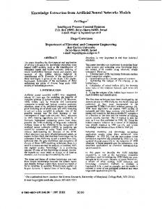
2.1.1 THE ARTIFICIAL NEURON – PROCESSING UNIT The basic processing element of an ANN is called artificial neuron, or simply neuron and it is a model based on the fundamental property of a biological neuron. According to Figure 2.1 the artificial neuron is composed of three functional elements: a set of synapses characterized by weights, a summing junction and an activation function. Input Signals x1 wj1

Bias

θj

x2

wj2 ...

.. .

xp

wjp

∑

rj

Activation Function

ϕ (.)

Output yj

Summing Junction

Synaptic weights Figure 2.1 - Artificial Neuron

The weights establish the particular connectivity between the signal source and the neuron. They are used to attenuate or amplify, by a weighting factor wij , the input signal xi coming from the environment or from other neurons. The weight wij is positive if the associated synapse is excitatory and it is negative if the synapse is inhibitory. The summing junction implements the weighted sum of the inputs according to the following expression: r j = ∑ wij x i + θ j p

i =1

(2.1)

where θ j is an externally applied bias that has the effect of increasing or lowering the summing junction signal. The activation function receives the signal of the summing junction and then calculates the internal stimulation or activation level of the neuron. Based on this level, the neuron may or may not produce an output. The relationship between internal activation level and output may be linear or non-linear. The activation function squashes the amplitude of the output in the range of [0 1], or alternately [-1 1]. Considering the activation function ϕ(.), the output of the neuron is calculated by: y j = ϕ ( ∑ wij xi + θ j ) p

i =1

(2.2)

7


The activation function is also known as transfer function; its three major types reported in the literature are: 1. Threshold Function. For this type of function, we have:

⎧⎪1 if r j ≥ 0 ϕ (r j ) = ⎨ ⎪⎩0 if r j < 0

(2.3)

2. Piecewise-Linear Function. This function is described by:

⎧1 ⎪ ϕ ( r j ) = ⎨r j ⎪ ⎩0

if r j ≥ 1 / 2 if 1/2 > r j > −1 / 2

(2.4)

if r j ≤ −1 / 2

3. Sigmoid Function. It is a strictly increasing function that exhibits smoothness and asymptotic properties: • Logistic Function. This sigmoid function, as showed in Figure 2.2a, is described by:

ϕ (r j ) =

1 1+ e

− ar j

(2.5)

where a is the slope parameter of the function. The function range is [0, 1]. • Hyperbolic Tangent Function. This sigmoid function, as showed in Figure 2.2b, is described

by:

ϕ (r j ) =

1− e

− ar j

1+ e

− ar j

(2.6)

where a is the slope parameter of the function. The function range is [-1, 1]. The sigmoid function is the most usual activation function in ANN and this is mainly due its differentiability property. As we will see in section 2.1.4, differentiability is an important feature of the neural network learning theory. According to common usage, a function g: ℜ →ℜ is called sigmoid if the following criterion is satisfied:

⎧lim r →−∞ g (r ) = 0 ( non - symmetric) or lim r →−∞ g ( r ) = −1 (anti - symmetric) ⎨ ⎩lim r →∞ g (r ) = 1

8

(2.7)


For the scope of this thesis, an unusual anti-symmetric sigmoid function in ANN is introduced. This function, which we have called basis-sigmoid function, obeys the criterion presented in 2.7. The basis-sigmoid function, as showed in Figure 2.3, is defined by: − ax ⎧ ⎪1 − e g ( x ) = ⎨ ax ⎪ ⎩e - 1

x≥0

(2.8)

x 0

10

m

p

j =1

i =1

(2.11)


This result was extended by Stinchcombe and White [4] who demonstrated that even if the activation function used in the hidden layer is a rather general nonlinear function, the same type of MLP is still a universal approximator. More or less at the same time, Funahashi [5], Cybenko [6], Kreinovichi [7] and Ito [8] proved similar results. In [9], the set of activation functions employed so far in [3] has been generalized. In this work it was demonstrated that if the activation function in (2.11) is continuous, bounded and non-constant, then a MLP using sufficiently many hidden neurons has the capacity to approximate arbitrarily well every f ∈ C ( I n ) . In [10] results were extended for the case when also squashing functions are used in the

output unit. Based on the universal approximator proofs, it was concluded that the approximation capability of the MLP is not dependent on the choice of a specific activation function, rather it is the MLP architecture itself which gives neural networks the potential to be universal approximators. Although MLP models are considered universal approximators, it is important to point out that the proofs presented in the literature previously mentioned are all existence proofs, i.e. they have proved that a MLP can find an input-output mapping using sufficiently hidden units, however they not reveal how to find the optimal ANN model - nothing is concluded about the number of necessary hidden neurons that will permit the ANN to find a good or better approximation of the problem. There are many works in the literature that deal with this problem – model selection and regularization of ANN. In section 2.1.5, this subject will be treated in more detail.

2.1.3 NEURAL NETWORK LEARNING According to Mendel and McClaren [11]: “Learning is a process by which the free parameters of a

neural network are adapted through a continuing process of stimulation by the environment in which the network is embedded. The type of learning is determined by the manner in which the parameter changes take place”. The ability to learn from examples is the most interesting property of a Neural Network and it is realized through an iterative process of adjustments applied to its synaptic weights and thresholds. In order to design a learning process, it is important first to have a model of the environment in which the ANN operates, i.e. we must know what information is available to the neural network. We refer to this model as a learning paradigm. In general there are two main learning paradigms, supervised learning and unsupervised learning.

11


In supervised learning, the outputs of the neural network are compared with the desired outputs or target outputs, and the error is calculated. The weights are adjusted so as to minimize this error. In unsupervised learning though, the weights are determined as a result of a self-organizing process, i.e. the connections to the network weights are not performed by an external agent. The network itself decides what output is best for a given input and reorganizes accordingly. Among the algorithms used to perform supervised learning, the Back-propagation algorithm has emerged as the most widely used and successful algorithm for the design of Multilayer Feedforward Networks.

2.1.3.1 BACK-PROPAGATION ALGORITHM The Back-propagation algorithm is of iterative type and based on the minimisation of a sum-squared error utilising gradient descent method. This learning algorithm is mainly composed of two phases: • Information flow in forward direction. In this phase, the activation of hidden neurons is

propagated to output neurons. Then, the error between the output values and the desired (target) values is calculated. • Information flow in backward direction. In this phase, the error is propagated in backward

direction and the weights connecting different levels of units are updated. During the learning process a set of input-output patterns is presented continuously to ANN in order to minimize the difference between target and network output values by means of modifying connection weights. Considering the ANN of the Figure 2.4, the error signal of the output neuron k in iteration n is calculated by:

e k ( n ) = d k (n ) − y k (n )

(2.12)

For all output neurons included in set C of the ANN, the instantaneous sum of squared errors of the network is given by: Ε (n ) =

∑e

k∈C

2 k (n )

(2.13)

and for all N patterns presented for ANN, the average squared error is defined by: Ε av =

12

1 N

∑ Ε(n) N

n =1

(2.14)


The average squared error E av is a function of all free parameters of the ANN (weights and bias) and it represents the cost function that has to be minimized during the learning process. The adjustment of the weights, in layer l, is performed according to the generalized delta rule: w (jil ) (n + 1) = w (jil ) ( n) + ηδ (j l ) ( n) y i(l −1) (n)

(2.15)

where η is the learning-rate parameter and δ (j l ) ( n) is the local gradient calculated by:

δ

(l ) j ( n)

⎡e (jL ) ( n ) g 'j (r j( L ) ( n)) = ⎢ ' (l ) ( l +1) ⎢ f j (r j ( n )) δ k (n)wkj(l +1) ( n) ⎢ ⎣

∑

for neuron j in output layer L for neuron j in hidden layer l

(2.16)

As we can see from (2.16), the main restriction to the function activation is that it has to be a differentiable function. As mentioned later, due its differentiable feature, the sigmoid function is the most used activation function in the hidden neurons. Let us consider, for the purpose of this thesis, a MLP with only one hidden layer and the sigmoid-basis defined in (2.8) as activation function of all hidden neurons. For the hidden neuron j, we have then:

⎧1 − e − r j ( n) ⎪ f j (r j ( n)) = ⎨ r ( n) ⎪⎩e j − 1

if r j ( n) ≥ 0 if r j ( n) < 0

(2.17)

Differentiating (2.17) with respect to r j (n) :

⎧⎪e − r j ( n) f (r j (n)) = ⎨ r ( n ) ⎪⎩e j ' j

if r j (n) ≥ 0 if r j (n) < 0

(2.18)

and as the output neuron is given by s j (n) = f j (r j ( n)) , we can express (2.18) as:

⎧⎪1 − s j ( n) f j' (r j ( n)) = ⎨ ⎪⎩1 + s j (n)

if r j (n) ≥ 0 if r j (n) < 0

(2.19)

Then, for a neuron in the hidden layer of the neural network, the local gradient is expressed by:

13


δ

∑ δ k (n)wkj (n)

if r j ( n) ≥ 0

∑ δ k (n)wkj (n)

if r j (n) < 0

⎡(1 − s j (n)) ⎢ k j ( n) = ⎢ (1 + s j (n)) ⎢ k ⎣

neuron j is hidden

(2.20)

We can see from (2.20) that if the basis-sigmoid function (or another sigmoid function) is used as activation function of hidden neurons, its derivative can be calculated simply from its output value, without the need of more complex calculations. This is very useful since it reduces the overall number of calculations needed to train the network. This is an important advantage of the use of general sigmoid function in Back-propagation algorithm. Another important advantage is restricted to a group of sigmoid functions. The basis sigmoid and the tangent sigmoid function are both anti-symmetric function, since they have the following property: f j (− r j ( n)) = − f j ( r j (n))

(2.21)

It has been shown that a Multilayer Neural Network trained with Back-propagation may, in general, learn faster when the sigmoid function used as activation function obeys (2.21) [2]. If a non-symmetric function is used as activation function of neurons located beyond the first hidden layer, the output of the neuron will be restricted to [0,1]. It can introduce a source of systematic bias for those neurons, whereas if an anti-symmetric function is used, the output can assume positive and negative values in the interval [-1,1]. It is likely for its mean to be zero. The use of non zero-mean input signals or non-zero induced neural output affect the eigenvalues of the Hessian matrix of the cost function E av (x) . The Hessian matrix is formed with the second derivative of

E av (x) with respect to the weight w. The learning time of the ANN is sensitive to λ max / λ min , where

λ max is the largest eigenvalue of the Hessian matrix and λ min is its smallest non-zero eigenvalue. For inputs with non-zero mean the ratio λ max / λ min is larger than for zero-mean values, then for the learning time (in terms of number of iterations) to be minimized the use of non-zero mean inputs should be avoided [2].

2.1.3.2 BACK-PROPAGATION – MODIFICATIONS AND EXTENSIONS The learning theory has to deal with three important issues: capacity, sample complexity and time complexity. The study of the learning capacity of the neural network is concerned with how much the network can learn from example; sample complexity refers to the number of random examples needed for the learning system to produce a hypothesis that is correct, and time complexity is interested in how fast the system can learn.

14


When we are talking about time complexity, it means computational complexity of the learning algorithm used to estimate a solution from training patterns. Many existing learning algorithms have high computational complexity, and the Back-propagation for Multilayer Feedforward Networks is a good example of it. Back-propagation is computationally demanding because of its slow convergence. To deal with this problem, in a few recent years, numerous modifications and extensions have been proposed for Back-propagation algorithm. It is worth specifying some of these methods: Back-propagation with momentum [12]: Although larger learning rates will result in more rapid learning, this also led to oscillation. The way to use larger learning rates without leading to oscillations is to modify (2.15) by adding a momentum term:

[

]

w (jil ) (t + 1) = w (jil ) (t ) + α w (jil ) (t − 1) + ηδ (j l ) (n) y i(l −1) (n)

(2.22)

where α is a small positive constant. A larger α increases the influence of the last weight change on the current weight change. Such modification in fact filters out the high-frequency oscillations in the weight changes since it tends to cancel weight changes in opposite directions and reinforces the predominant direction of change. Quickprop Algorithm [13]: This is a so-called second-order learning algorithm, which uses an interpolation method to estimate more accurately the error minimum for each weight. In this method, the basic idea is to estimate weight changing by assuming a parabolic shape for the error surface. The weights changes are then modified by the use of heuristic rules to ensure downhill motion at all spaces. RPROP Algorithm (Resilient Back-propagation) [14]: This method is called resilient because it uses the local topology of the error surface to make a more appropriate weight change. In other words, we introduce a personal update value for each weight, which evolves during the learning process according to its local view of the error function. It is very powerful and efficient because the size of the weight step taken is no longer influenced by the size of the partial derivative. It is only determined by the sequence of the signs of the derivatives, which provide a reliable hint about the topology of the local error function. Levenberg-Marquardt Algorithm [15]: This optimization technique is more powerful than gradient descent, but requires more memory. For this algorithm the performance index to be optimized is defined as: F (w ) =

∑ ⎡⎢⎣∑ (d P

K

p =1

k =1

⎤

kp

− o kp ) 2 ⎥ ⎦

(2.23)

15


where w = [w1 w2 ... w N ] is the vector of all weights of the ANN, d kp is the desired output of T

the k-th output neuron and the p-th pattern, o kp is the actual value of the k-th output neuron and the p-th pattern, N is the number of the weights, P is the number of patterns, and K is the number of the output neurons. The equation (2.23) can be written as: F (w) = E T E

(2.24)

with E = [e11 ...ek 1 e12 ...e K 2 ...e1 P ...e KP ]

T

(2.25)

e kp = d kp − o kp , k = 1,..., K , p = 1,..., P

where E is the cumulative error vector (for all patterns.) From (2.25) the Jacobian matrix is defined as:

J=

K δδwe K δδwe M M M δe δe K δw δw M M M δe δe K δw δw δe δe K δw δw M M M δe δe K δw δw

⎡ δe11 ⎢ δw ⎢ 1 ⎢ δe21 ⎢ δw ⎢ 1 ⎢ ⎢ ⎢ δeK 1 ⎢ δw 1 ⎢ ⎢ ⎢ δe ⎢ 1P ⎢ δw1 ⎢ δe ⎢ 2P ⎢ δw1 ⎢ ⎢ ⎢ δe KP ⎢ δ w ⎢ 1 ⎣

δe11 δw2 δe21 δw2

⎤ ⎥ N ⎥ ⎥ 21 ⎥ N ⎥ ⎥ ⎥ K1 ⎥ ⎥ N ⎥ ⎥ ⎥ 1P ⎥ N ⎥ ⎥ 2P ⎥ ⎥ N ⎥ ⎥ ⎥ KP ⎥ ⎥ N ⎦ 11

K1 2

1P 2

2P 2

KP 2

(2.26)

The Jacobian matrix contains the first derivatives of network errors with respect to the weights. The weights are calculated by:

16


wt +1 = wt − (J Tt J t + α t I ) J Tt E t −1

(2.27)

where I is the identity matrix, α is a learning parameter and J is a Jacobian of m output error with respect to n weights of the ANN. The parameter α is automatically adjusted, at each iteration, in order to assure convergence. If α is very large, the above expression approximates gradient descent. For small values of α the above expression tends to the Gauss-Newton method.

2.1.4 GENERALIZATION One of the major advantages of an ANN is its ability to generalize. The neural network works well if it has a good generalization ability, i.e. it is able to perform good predictions in front of new input values, which are not part of the training pattern but are generated by the same input/output distribution underlying the training data. However, neural networks can suffer from either underfitting or overfitting [16] and in these cases, ANNs exhibit poor generalization performance. To better understanding underfitting and overfitting, the bias/variance dilemma has to be introduced. THE BIAS-VARIANCE DILEMMA Let consider the expression for the expected value of the sum-of-square error (SSE) function: E

{[y( x) − t | x ] } 2

(2.28)

where E[.] is the expected value of the argument, y(x) is the output of the neural network for a given input vector x, and t | x is the conditional average of the target vector (output desired) given an input vector x. The equation (2.28) can be rewritten as: E

{[y( x) − t | x ] }= E {[y( x) − E{ y( x)}] }+ [E{ y( x)} − t | x ] 2

2

2

(2.29)

The first term on the right-hand side is the variance of y given x, and the second term is the squared bias of the expected value of the SSE of the network output. The variance represents the average sensitivity of the neural network mapping y(x) to a particular training set, i.e. it represents how sensitive the ANN mapping is to different data patterns, by measuring the expected error between the average target and an ANN model identified on a single data

17


pattern. The variance term can indicate the excessive complexity of the class of models. This means that a class of too powerful ANN models runs the risk of being excessively sensitive to the noise affecting the training pattern. The bias represents the difference between the target (actual) output of the network, t, given a set of input, and the average of the neural network mapping y(x). The bias term permits one to measure how closely the average guess of the learning ANN matches the target. Hence, the bias represents the inability of the derived model y(x) to accurately approximate the target. If, on the average, the ANN model is different from the target, then the model is said to be a biased estimator of the target. Conversely, if the model output converges to the target output the model is said to be unbiased, i.e. it matches the target well [18]. When we have a large generalization error due to a large model bias, we speak of underfitting. This means that the complexity of the network (in terms of the number of hidden nodes and weights) is lower than the complexity of the phenomenon being modeled. When we have a large generalization error due to a large model variance, then we speak of overfitting. This means that the network complexity exceeds the complexity of the phenomenon being modeled. The optimal model, with respect to training data size and generalization error, is between these two extremes and, in practice, a balance between bias and variance should be found. The trade-off between the bias and the variance contributions to the generalization error is known as the bias/variance dilemma. The bias/variance tradeoff for finite training sets as a function of the model size is illustrated in Figure 2.5.

Error

High Bias Low Variance Underfitting

Low Bias High Variance Overfitting

Test set Training set Best model

Model size

Figure 2.5-The bias/variance Trade-off

In the last few years, a number of methods have been developed to improve generalization accuracy. These methods generally fall into two main categories: model selection and regularization methods. Model selection is concerned with the numbers of layers in the neural network, the number of neurons in each layer and, the interconnection between the neurons. For any given problem there is an

18


essentially infinite number of possible MLP architectures, but only a small subset of these exhibit good performances in general. We have to choose a proper size for the network, large enough that it will fit well, but small enough to minimize overfitting. Regularization involves constraining or penalizing the solution of the estimation problem to improve network generalization ability by smoothing the predictions [19]. There are several methods used for model selection and regularization of neural networks. We will briefly discuss some of these strategies here, the remaining ones can be found in [2] and [20]: • Weight decay. It is a regularization method that penalizes large weights. The weight decay

penalty term causes the insignificant weights to converge to zero. This produces a network that has fewer free parameters, which in theory should result in better generalization. It can be realized by adding to the cost function a term that penalizes large weights: E (W ) = E 0 (W ) +

1 λ 2

∑w

2 i

(2.30)

i

where E0 is the sum of squared errors, λ is a parameter governing how strongly large weights are penalized, W is the vector containing all free parameters of the ANN. • Cross validation [21]. In this method, the data set is divided into two subsets: training and

testing set (typically 25-35% of the data set). The test set is not used until all training is done. The performance on this test data will be an unbiased estimate of the generalization error, provided that the data has not been used in any way during the modeling process. • Early-stopping. It is a form of regularization used when an ANN is trained by gradient

descent. In this method, the data set is divided into three subsets: training, validation and testing set. The gradient descent is applied to the training set and then the network weights and biases are updated. After each sweep through the training set, the network is evaluated on the validation set with the objective of monitoring the validation error. If this error begins to rise, this generally indicates overfitting and the training will stop. The network with the best performance on the validation set is then used for actual testing set. The learning algorithm choice to training the MLP has to move reasonably slowly towards the minimum of the training error function. (The reason for this is that, if a very fast learning algorithm such as Levenberg-Marquardt method is employed, which reaches the minimum in very few iterations, there is not much chance of stopping at the right location away from the minimum where validation error is the smallest.) A method such as RProp or QuickProp

19


may be very well suited for early stopping. Early stopping is very common practice in neural network training and often produces networks that generalize well. • Hints [22]. Incorporation, during the learning, of prior information about the target function

beyond the available input-output examples. With hints, the performance of learning model can be improved by reducing capacity without sacrificing approximation capabilities.

2.1.5 RADIAL BASIS FUNCTION NETWORKS After MLP network, the Radial Basis Function Network (RBF) comprises one of the most used ANN models. The RBF was proposed by Moody and Darken [23] [24] and it is a network structure that employs local receptive fields to perform functions mapping. Figure 2.6 illustrates a RBF network.

Receptive field units

ϕ 1 (.)

x1

ϕ 2 (.)

x2 . . .

. . .

xn

w1 w2

∑

→

f ( x)

wN

ϕ N (.) Figure 2.6-Radial Basis Function Network

Generally, an RBF network with a single output can be expressed as follows: ⎛ ⎜ → N ⎛ ⎞ f ⎜ x ⎟ = ∑ wi ϕ i ⎜ ⎜ ⎝ ⎠ i =1 ⎜ ⎝

→

→

⎞

x − ci ⎟ →

σi

⎟ ⎟ ⎟ ⎠

(2.31)

→

→

where ϕi (.) is called the i-th radial basis function or the i-th receptive field unit, c i and σ i are the

center and the variance vectors of the i-th basis function and wi is the weight or strength of the i-th receptive field unit. Typically, the function ϕi (.) is chosen as a Gaussian function:

20


⎡ ⎢− → ⎛ ⎞ ϕ i ⎜ x ⎟ = exp ⎢ ⎢ ⎝ ⎠ ⎢ ⎣

→

→

2

x − ci

σ i2

⎤ ⎥ ⎥ ⎥ ⎥ ⎦

(2.32)

→

Thus, the radial basis function ϕi ⎛⎜ x ⎞⎟ computed by i-th receptive field is maximum when the input ⎝ ⎠

→

→

vector x is near the center c i of that unit. When lateral connections are added between the receptive filed units, the network can produce the normalized response function as the weighted average of the strengths: →

∑ wiϕi ⎛⎜ x ⎞⎟ N

→

⎛ ⎞

f ⎜ x⎟ = ⎝ ⎠

i =1

⎝ ⎠ →

∑ ϕi ⎛⎜ x ⎞⎟ i =1 ⎝ ⎠ N

(2.33)

Several supervised and unsupervised learning methods have been developed to find optimal values of the RBF network parameters [23] [25-27]. RBF have been successfully applied to a large diversity of applications including interpolation, chaotic times-series modelling, system identification, control engineering and other.

2.2 FUZZY SYSTEMS Fuzzy Logic, which was conceived by Lotfi Zadeh in the 1960s, consists of a variety of concepts and techniques for representing and inferring knowledge that is imprecise, uncertain, or unreliable. The introduction of this new theory has improved the traditional idealistic mathematical approach. The new concepts and ideas behind Fuzzy Logic have led to more realistic and accurate mathematical representations of the perception of truth, where perception refers to the human brain and its way of observing and expressing reality. Fuzzy logic addresses the imprecision of the input and output variables of the system by defining fuzzy numbers and fuzzy sets that can be expressed in linguistic variables (e.g. small, medium and large). The fuzzy sets are combined with fuzzy rules that are obtained from human experts or based on domain knowledge. The obtained collection of if-then rules is combined into a single system. Different fuzzy systems use different principles for this combination. There are three types of fuzzy systems that are commonly used in the literature: pure fuzzy systems, Takagi-Sugeno Systems and fuzzy systems with fuzzifier and defuzzifier (Mamdani Systems).

21


The Takagi-Sugeno System is the model of interest of this thesis and it will be described in more detail. Let us start with some basic concepts in Fuzzy Systems that are important in the development of the methodology of extraction of rules from ANN proposed in this work.

2.2.1 FUZZY SET THEORY Definition 2.1: Fuzzy Sets

Fuzzy sets are a generalization of classical crisp sets. They are functions that map a value or a member of the set to a number between zero and one indicating its actual degree of membership. Let U be a nonempty set, called the universe, whose elements are denoted by x. The fuzzy set A in U is characterized by a membership function:

µ A ( x ) : x → [0 1]

(2.34)

The Fuzzy set A may be also represented as a set of ordered pairs of a generic element x and its membership value, that is: A = {(x, µ A ( x ) ), x ∈U }

(2.35)

The geometrical shape of a membership function is the characterization of uncertainty in the corresponding fuzzy variable. The triangular membership function is the most frequently used function and the most practical. Other shapes such as trapezoid, s-function, pi-function and z-function are also used. Definition 2.2: Linguistic Variable.

A linguistic variable is a variable that can take words in natural language as its values and the words are characterized by fuzzy sets defined in the universe of discourse in which the variable is defined [28]. It is characterized by (X, T, U, M), where X is the name of the linguistic variable; T is the set of linguistic values that X can take; U is the actual physical domain in which the linguistic variable takes its quantitative values and; M is a semantic rule that relates each linguistic value in T with a fuzzy set in U. The concept of linguistic variable allowed the introduction of human knowledge into systems in a systematic and efficient manner. The linguistic variable allows formulating vague descriptions in natural languages in precise mathematical terms.

22


In Figure 2.7 an example of three fuzzy sets is given in the universe of discourse U representing the interval of possible concentration values of gas H2 dissolved in oil of a transformer. “Concentration” is the linguistic variable with three terms “Small”, “Medium”, and “High” represented by fuzzy sets with the membership functions shown in the figure.

µ (concentration) Small

Medium

10

50

High

100 Concentration ( ppm)

Figure 2.7 –Fuzzy sets to gas concentration

Definition 2.3: Linguistic modifiers or hedges.

Operators that alter the membership functions for the fuzzy sets associated to the linguistic labels. The meaning of the transformed set can easily be interpreted from the meaning of the original set. A short list of linguistic hedges and their somewhat standard role in fuzzy logic are listed in Table 2.1. Table 2.1 – Linguistic hedges Hedges

Function

Very, extremely

Concentration

Somewhat

Dilution

Definitely, nearly

Intensification

More or less

Relaxation

Not

Negation

Below, above

Restriction

In figure 2.8 example of concentration hedge for the fuzzy set “small” is shown

23


µ (concentration) Extremely small Very small Small

10

25

50

Concentration ( ppm)

Figure 2.8 – Concentration hedges for “small”

Definition 2.4: Fuzzy Union – The S-norms

Considering s : [0,1] × [0,1] → [0,1] as mapping that transform the membership functions of fuzzy sets A and B into the membership function of the union of A and B, that is, s[µ A ( x), µ B ( x)] = µ A∪ B ( x ) . The function s is qualified as an union fuzzy or s-norm if at least it satisfies the following requirements: 1) s (1,1) = 1, s(0, a ) = s (a,0) = a (boundary condition) 2) s (a, b ) = s (b, a) (commutative condition) 3) If a ≤ a´ and b ≤ b´, then s (a, b) ≤ s( a´, b´) (non-decreasing condition)

4) s (s( a, b), c ) = s (a, s(b, c )) (associative condition). Table 2 .2 list some S-norms proposed in the literature. Table 2.2 – S-norms S-norm Einstein sum

Drastic sum

24

s ( a , b) =

a+b 1+ a + b

⎧a if b = 0 ⎪ s (a, b) = ⎨b if a = 0 ⎪1 if otherwise ⎩

Algebraic sum

s (a, b) = a + b − ab

Maximum

s (a, b) = max( a, b)


Definition 2.5: Fuzzy Intersection – The T-norms Considering t : [0,1] × [0,1] → [0,1] as a mapping that transform the membership functions of fuzzy sets

A and B into the membership function of the intersection of A and B, that is, t [µ A ( x ), µ B ( x )] = µ A∩ B ( x) . The function t is qualified as an intersection fuzzy or t-norm if at least it satisfies the following requirements: 1) t (0,0 ) = 0, t ( a,1) = t (1, a) = a (boundary condition) 2) t (a, b ) = t (b, a) (commutative condition) 3) If a ≤ a´ and b ≤ b´, then t (a, b) ≤ t (a´, b´) (nondecreasing condition) 4) t (t (a, b), c ) = t (a, t (b, c)) (associative condition). The table 2 .3 list some T-norms proposed in the literature. Definition 2.6: Fuzzy Complement

Consider c : [0,1] → [0,1] as a mapping that transforms the membership function of fuzzy set A into the membership function of the complement of A, that is, c[µ A ( x)] = µ A ( x ) . The function c is qualified as a complement fuzzy if at least it satisfies the following requirements: 1) c(0) = 1 and c (1) = 0 (boundary condition) 2) For all a, b ∈ [0,1], if a < b then c( a) ≥ c(b) (nonincreasing condition), where a and b denote membership of some fuzzy set, say, a = µ A ( x) and b = µ B ( x) . Table 2.3 – T-norms T-norm Einstein product

Drastic product

t ( a, b ) =

ab 2 − (a + b − ab)

⎧a if b = 1 ⎪ t ( a, b) = ⎨b if a = 1 ⎪0 otherwise ⎩

Algebraic product

t ( a, b) = ab

Minimum

t ( a, b) = min( a, b)

25


Definition 2.7: Associated class – DeMorgan’s Law

For each S-norm there is a T-norm associated with it, where associated means that there is a fuzzy complement such that the three together satisfy the DeMorgan’s Law. Specifically, the S-norm s (a, b) , T-norm t ( a, b) and fuzzy complement c (a ) form an associated class if : c[s( a, b)] = t [c( a), c (b)]

(2.36)

Definition 2.8: Fuzzy Rule Base

A fuzzy rule base consists of a set of fuzzy IF-THEN rules that specify a linguistic relation between the linguistic label of input and output variables of the system. It is the heart of the fuzzy system in the sense that all other components are used to implement these rules in a reasonable and efficient manner. Specifically, the fuzzy rule base comprises the following fuzzy IF-THEN rules: Rule R 1 : IF x1 is A11 and ... x n is An1 THEN y is B 1

.. . Rule R m : IF x1 is A1m and ... x n is Anm THEN y is B m

(2.37)

where Ai and B are fuzzy sets in U ⊂ ℜ and V ⊂ ℜ , respectively, and X = ( x1 , x 2 ,...x n ) ∈U and y ∈V are the input and output of the fuzzy system respectively.

The IF part of a rule is called premise or antecedent, while the THEN part is called conclusion or consequent of the rule.

2.2.2 FUZZY RULE-BASED SYSTEM A Fuzzy-rule-based system also known as Fuzzy Inference System (FIS) is composed of four functional blocks, as shown in Figure 2.9: • Fuzzification. Normally, the inputs to the fuzzy system are crisp values and thus these have to

be converted to fuzzy sets. The fuzzification block transforms the crisp inputs into degrees of matching with linguistic values. • Database and Rule base. The database defines the membership functions of the fuzzy sets used

in the fuzzy if-then rules that compose the rule base. Usually, the rule base and the database are jointly referred to as the knowledge base. • Inference Engine. It performs the inference on the fuzzy rules and produces a fuzzy value for

the output of the system.

26


• Defuzzification. Converts a set of fuzzy variables into crisp values in order to enable the output

of the fuzzy system to be applied to another non-fuzzy system.

Input

Fuzzification

Fuzzy

crisp

Inference Engine

Fuzzy

Output Defuzzification crisp

Database Rule base

Figure 2.9 – Schematic diagram o Fuzzy Rule-based System

2.2.3 TAKAGI-SUGENO FUZZY MODEL The Fuzzy Inference System can be categorized into two families: 1) The family that includes linguistic models based on collections of IF-THEN rules, whose antecedents and consequents utilize fuzzy values such as Mamdani fuzzy inference, and 2) The family that uses a rule structure that has fuzzy antecedent and functional (crisp) consequent. The second family, based on Takagi-Sugeno (TS) fuzzy inference systems, is built with rules in the following form: Rule R j : IF x1 is A1 j AND … AND x n is Anj THEN y j = g ( x1 ,..., x n )

(2.38)

where Aij is a fuzzy set and xi is the input of the system. The consequent of the rule is an affine linear or non-linear function of the input variables. The Sugeno fuzzy model was proposed by Takagi, Sugeno, and Kang [29] in an effort to formalize a system approach to generating fuzzy rules from an input-output data set. The Sugeno fuzzy model is also known as Takagi-Sugeno-Kang model (TSK). When y j is a first-order polynomial, we have the first-order Takagi-Sugeno fuzzy model. When y j is a constant, we then have the zero-order TakagiSugeno fuzzy model, which can be viewed as a special case of the Mamdani fuzzy inference with consequent as a singleton. The zero-order Takagi-Sugeno fuzzy model is built with rules in the following form: Rule R j : IF x1 is A1 j AND… AND x n is Anj THEN y j = c j

(2.39)

27


The firing strength of each rule is calculated by: n

v j = ∩ µ ij ( x i )

(2.40)

i =1

where µ ij ( x i ) is the membership function associated to the fuzzy set Aij and ∩ represent the product operator (AND operator). The output of the system is computed as the weighted average of the y j , that is:

∑y v f ( x) = ∑v N

j =1

j

j

(2.41)

N

j

j =1

where N is the number of rules of the system. The output can be also calculated by: f ( x) =

∑y v N

l =1

j

(2.42)

j

The Figure 2.10 illustrates the reasoning mechanism for a zero-order TSK, which is the model of interest of this thesis

A1

B1

THEN

and

IF

v1 y1=c1

x1

x2

B2

A2 IF

v2

and

y2=c2 x1

x2

y=

v1 y1 + v2 y2 = v1 y1 + v2 y2 v1 + v2

Figure 2.10 – Zero-Order Takagi-Sugeno Fuzzy Model

28


2.2.4. FUZZY SYSTEM INTERPRETABILITY AND TRANSPARENCY A Fuzzy System has as a most important property, which distinguishes it from other techniques such as neural networks, its capacity of explanation. Fuzzy systems have the potential to express the behavior of the real systems in a comprehensible manner, i.e. FIS are systems that have interpretability. However, such interpretability is valid only if the fuzzy system satisfies the conditions of transparency. Fuzzy transparency is directly associated to the concept of linguistic interpretability. However, transparency and interpretability are distinct terms. Interpretability is a property that exists by default being associated with linguistic rules and fuzzy sets, whereas transparency is the measure of how valid is the linguistic interpretation of the system and it is not a default property [30]. When a fuzzy system is built based on expert knowledge, the transparency condition can be easily satisfied. However, when the fuzzy system is built directly from data and, generally, the system accuracy is the mainly objective, the transparency is generally lost leading to results that can be considered black-box systems, which do not provide any meaningful linguistic meaning. If transparency is ignored during the process of building fuzzy systems, this important advantage of fuzzy systems over neural networks and other conventional techniques is lost completely. According to [30], a fuzzy system is transparent only if all rules of the rule base are transparent. The rule of the fuzzy system is considered transparent, if its firing strength n

v j = ∩ µ ij ( x i ) = 1 i =1

(2.43)

has as consequence the following output for the system: y = yj

(2.44)

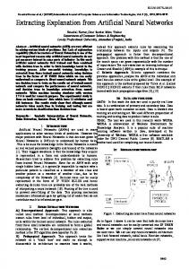
where y j is the center of the output membership associated with the rule j. For the case of zero-order Takagi-Sugeno model, y j is the constant consequent. The transparency conditions are defined based on the overlapping degree of the inputs membership functions and the symmetry of the output membership. For the fuzzy system to be transparent, the overlapping of the inputs membership functions has to be smaller than 50%. It will guarantee the existence of transparency checkpoints, which are points in input-output space where the explicit contribution of a given rule takes place and the rule under observation is fully activated. Figure 2.11 gives an example of transparent fuzzy system [30], where the asterisks denote transparency checkpoints.

29


-3

4

-2

-1

0

1

2

3

4

5

6

7

x2

8

*

3 2

*

*

1 0

*

-1 -2

*

-3

x1

0

2

4

y

6

Figure.2.11 - Transparent fuzzy system

If the overlapping is greater than 50%, however, at least two rules contribute simultaneously for any given input, thus output is always the result of interpolation. This makes the contribution of a given rule invisible in system output and thus the fuzzy system may not be considered transparent. Figure 2.12 gives an example of a non-transparent fuzzy system [30].

-3

4

-2

-1

0

1

2

3

4

5

6

7

8

x2

*

3 2

*

*

1 0 -1

*

*

-2 -3

x1

0

2

4

6

y

Figure 2.12 - Non-transparent fuzzy system

It is important to point out that if the fuzzy system works with membership functions with infinite support, such as Gaussian functions, the overlapping measure cannot be directly applied. For these cases, we have to re-define the condition of transparency using α-cuts. Despite the insufficient attention given to this topic, some algorithms have been developed with the aim of guaranteeing the transparency of fuzzy systems. Generally, the transparency is guaranteed by imposing constraints on membership functions or by using special membership functions that make transparency a default property of a fuzzy system. Some works in this area can be found in [30-32].

30


It is important to point out that transparency protection generally deteriorates the approximation capacities of the fuzzy learning algorithm. However, it is not a surprise since the trade-off between accuracy and transparency is a long known fact. Besides transparency, there are other factors that may affect the interpretability of fuzzy systems. In the last few years some proposals related to interpretability improvement of a fuzzy system have been developed. It is worth to present some of them: • Input variables selection. The rule base of the fuzzy system grows exponentially with the

number of inputs. So, for problems with a large number of inputs and consequently a large rule base, the readability of the fuzzy system cannot be guaranteed. To solve this problem, a variable selection process with the aim of reducing the number of variables is a good choice. Some works have been developed to select input variables in the model [33-35] and to select input variables in the linguistic rules [36] [37]. • Merging/Selecting Rules. Generally, in a rule base with excessive size we can have:

redundant rules, erroneous rules and conflictive rules. This can affect the interpretability of the fuzzy system. To solve this problem, some works based on rule reduction have been developed. Two rule reduction approaches can be distinguished: 1. Selecting Linguistic rules. Selection of a subset of the rules from a previous base rule through a search algorithm [38-40]. 2. Merging Lingusitic Rules. Through this method, the rule base can be reduced by merging the existing linguistic rules. In [41] a measure of similarity between fuzzy sets is used to quantify the similarity between fuzzy sets in the rule base. The measure of similarity is used to remove rules or merge rules. Others interesting works are [42], [43]. • Linguistic approximation. This method is used to derive a qualitative model from a fuzzy

model. The linguistic approximation is performed in the fuzzy set that is approximate to a word or phrase out of a given set of words using linguistic terms, hedges and connectives. During this process, a certain accuracy of the output fuzzy can be lost. The linguistic approximation is based on the similarity measure between fuzzy sets, such as:

S ( N , L) = N ∩ L / N ∪ L where

(2.45)

. is the cardinality of the fuzzy set, and N and L are fuzzy sets.

31


The linguistic approximation can be considered on three levels: 1. Approximation with linguistic terms 2. Approximation with linguistic terms and hedges 3. Approximation with linguistic terms, hedges and connectives As an example of linguistic approximation of a fuzzy set, let us follow the one presented in [44]. Consider two fuzzy sets N and L as shown in Figure 2.13. µ(x)

N

L

x

Figure 2.13 – Two Fuzzy set N and L

Figure 2.14 shows some possible linguistic terms that can be used to approximate N and L. µ(x)

calm soft

moderate

hard

zero

strong

x

Figure 2.14 – Possible Linguistic terms

Table 2.4 shows the linguistic approximation of N and L according to three levels of approximation. The measure of similarity S between the sets is also shown. Table 2.4 Results of Linguistic approximation

32

Level

Linguistic Expression

S

1

calm

0.62

2

Less than soft

0.87

3

More or less calm or more or less soft (Membership N)

0.94

Level

Linguistic Expression

S

1

moderate

0.76

2

More or less moderate

0.81

3

Not strong but more or less moderate (Membership L)

0.86


Some examples of methods that improve the transparency of the fuzzy model with linguistic approximation can be found in [44]-[46].

2.3 – FUZZY SYSTEMS VERSUS NEURAL NETWORKS Despite of their different origins, Fuzzy Systems and Neural Networks are two approaches that have many similarities. The most obvious similarity between them is the capacity to handle extreme nonlinearities in the system. Other similarities that can be highlighted are that they both: • are highly parallel structures; • do not require a mathematical model of the system; • have fault tolerance capabilities; • can generalize; • are universal approximators.

However, besides these common similarities that are considered as advantages of both approaches, neural networks and fuzzy system also have some individual advantages and drawbacks.

2.3.1 FUZZY SYSTEM ADVANTAGES AND DRAWBACKS Fuzzy systems are systems that have precisely the desired characteristics of an explicit form of knowledge. They are systems able to treat the uncertain and imprecise information. They can model the qualitative aspects of human knowledge employing fuzzy if-then rules, with fuzzy antecedents and consequents. However, problems arise when fuzzy systems have to be built. This is not always a straightforward task. Some difficulties of fuzzy system design that greatly restrict their application domain are: • There is no universal systematic method for the transformation of expert knowledge or

experience into the rule base of a fuzzy inference system; • Even when human specialists exist, their knowledge is often incomplete and episodic rather

then systematic; • A Fuzzy system that is built based only on knowledge will usually not perform as required.

During the design stage the expert can fail in specifying characteristic points, the number of rules, or the degree of “indistinguishability” in certain areas of the data space, and then a tuning process must usually be added so as to minimize the discrepancy between the model output and desired output. The tuning process results in modifying the membership function

33


and/or the rule base of the fuzzy system. This tuning process can be very time–consuming and error-prone. It is therefore useful to support the design process by automatic learning approaches that can make use of available data samples. • They suffer of the curse of dimensionality problem, meaning that the number of rules of the

system grows exponentially when the number of inputs increases and computational complexity in the implementation for practical problems increases accordingly.

2.3.2 NEURAL NETWORK ADVANTAGES AND DRAWBACKS Neural Networks present as main advantage their capacity of learning from examples. These systems, which rely on a distributed knowledge representation, are able to develop a concise representation of complex concepts. They can provide noise resistance and can adapt to unstable and largely unknown environments as well. The ANN knowledge is acquired during the training process through the presentation of a data set representative of the system while many fuzzy systems are built based on human knowledge (but remember that Takagi-Sugeno Systems may be built based on a learning process just like ANN). This is an important advantage of the ANN over Fuzzy Systems since it is know that it is almost impossible for an expert to describe his domain specific entirely in form of rules or other knowledge representation schemes. However, to provide the ANN with enough information (knowledge), the training set must be adequate (consistent) and sufficient. Despite of the proven capabilities of Artificial Neural Networks, this approach also has some drawbacks that lead to a barrier to a more widespread acceptance of them, mainly in industry area. One of the major drawbacks of the ANNs is the lack of capability to explain, in a humancomprehensible form, how they arrive at a particular decision. In most of the real world applications (especially in safety critical applications) it is necessary, namely in order for the specialist to gain more confidence in the system, to know the reasoning behind the conclusion of the ANN. However, explaining the behavior of the ANN is not an easy task since they have a distributed knowledge representation [47]. The knowledge learned by the neural networks is encoded in the parameters associated with the network connections, i.e. the weights and bias and these values usually are not meaningful for humans. In recent years, a number of works have been developed with the aim of re-addressing this general problem of explanation capability. In particular, a substantial part of these works have focused on a line of investigation involving the development of techniques for rule extraction from trained neural networks. As this thesis is concerned with this subject, rule extraction from neural networks will be described in the next chapter in more detail.

34


2.4 CHAPTER CONCLUSION This chapter reviewed some import definitions and concepts of neural networks and fuzzy systems. Emphasis was given for Zero-order Takagi-Sugeno Fuzzy systems and Multilayer Feedforward Neural Networks, since these issues are related to the methodology presented in this work. As far as the rule extraction from neural network is concerned, the basis-sigmoid function, which represents the base for all extraction process proposed in this work, was defined and presented. This concept will be used at later stages. As previously mentioned, one of the main objectives of this thesis is to extract rules that are entirely interpretable for human beings. The approach considered in this work uses the concept of approximation linguist after the rule extraction process to carry out this task and, for this purpose, the transparency property of fuzzy systems, as well as the concept of linguistic approximation were also discussed in this chapter. A comparison between Fuzzy Systems and Neural Networks was carried out in the final section of this chapter, in which some advantages and drawbacks of such systems were highlighted. The purpose is to make the reader aware of the interest in establishing relationships between ANN and FIS and in generating rule systems with the property of transparency. If this objective is achieved, and transparent rule bases are built from ANNs, one is ready to make explicit the hidden knowledge in Artificial Neural Networks.

2.5 CHAPTER REFERENCES [1] L. A. Zadeh , Fuzzy logic, neural networks and soft computing, One-page course announcement of CS 294-4, Spring 1993, University of California at Berkeley, November. [2] S. Haykin, Neural Networks. A Comprehensive Foundation, New Jersey: Prentice Hall. [3] K. Hornik, M. Stinchcombe, and H. White, “Multilayer feedforward networks are Universal Approximators”, Neural Network, Vol. 2, pp 359-366, 1989. [4] M. Stinchcombe and H. White, “Universal Approximation using feedforward networks with nonsigmoid hidden layer activation functions”. In Porccedings of the International Joint Conference on Neural networks, pp 613-618, San Diego, 1989. [5] K–I Funahashi, “On the approximate realization of continuous mapping by neural networks”, Neural networks, Vol. 2, pp183-192, 1989. [6] G. Cybenko, “Approximation by superposition of sigmoidal functions”, Mathematics of Control, Signal and Systems, Vol. 2, pp 303-314, 1989.

35


[7] V. Y. Kreinovich, “Arbitrary nonlinearity is sufficient to represent all functions by neural networks: a theorem”, Neural Networks, Vol. 4, pp. 381-383, 1991 [8] Y. Ito, “Represntation of functions by superpositions of a step or sigmoidal function and their applications to neural networks theory”, Neural Networks, Vol. 4, pp 385-394, 1991 [9] K. Hornik, “Approximation Capabilities of Multilayer Feedforward Networks”, Neural Networks, Vol. 4, pp. 251–257, 1991. [10] J. L. Castro, C. J. Mantas and J. M. Benitez, “Neural networks with a continuous squashing function in the output are universal approximators”. Neural Networks, Vol. 13, pp. 561-563, 2000. [11] J. M. Mendel and R. W. Mclaren, “Reinforcement learning control and pattern recognition systems”, In Adaptative, learning and Patter Recognition Sytems: Theory and Applications, New York: Academic Press, 1970. [12] D. E. Rumelhart, G. E. Hinton and R. J. Willians , Learning Internal Representations by Error Propagation. In [Rummelhart and McClelland, pp. 318-362, 1986. [13] S. E. Fahlman, “An Empirical Study of learning Speed in Back- Propagation Networks”, CarnegieMellon Computer Science Rpt. CMU-CS-88-162, 1988. [14] M. Riedmiller and H M Braun, “A Direct Adaptive Method for Faster Back-propagation Algorithm Learning: The RPROP Algorithm”, In: Proc. of IEEE Int Conf. on Neural Networks (ICNN), pp 586-591, San Francisco, 1993. [15] M. T. Hagan and M. Menhaj, “Training feedforward networks with the marquardt algorithm”, IEEE transaction on Neural Networks, Vol. 5, No. 6, pp 989-993, 1994. [16] M. Smith, Neural Networks for StatisticalModeling, International Thomson Computer Press, Boston, MA, 1996. [17] S. Geman, E. Bienenstock, and R. Doursat, “Neural Networks and the Bias/Variance Dilemma”, Neural Computation, Vol. 4, pp. 1-58, 1992. [18] Giovanna Castellano, A Neurofuzzy Methodology for Predictive Modeling, PhD. Thesis, University of Bali, Faculty of Science, November 2000. [19] L. K. Hansen and C. E. Rasmussen, “Pruning from Adaptive Regularization”, Neural Computation, vol. 6, No. 6, pp. 1222-1231, 1994. [20] C. M. Bishop, Neural Networks for Pattern Recognition. Oxford, UK: Clarendon Press, 1990. [21] M. Stone, “Cross-validatory choice and assessment of statistical predictions”, Journal of the Royal statistical Society B, Vol. 36, pp 111-147, 1974. [22] Y. Abu_Mostafa, “Learning from Hints in Neural Networks”, Journal of Complexity 6, 192-198, 1990.

36


[23] J. Moody and C. Darken, “Learning with localized receptive fields”, In D. Touretzky, G. Hinton, and T. Sejnowski editors, Porc. Of the 1988 Connectionist Models Summer School, Carnegie Mellon University, Morgan Kaufmann Publishers, 1988. [24] J. Moody and C. Darken, “Fast Learning in networks of locally-tuned processing units”, Neural Computation, Vol. 1, pp 281-294, 1989. [25] S. Chen, C.F.N Cowan and P. M Grant, “Orthogonal least squares learning algorithm for radial basis function network”, IEEE Trans. On Neural Network, Vol. 2, No.2, pp 302-309, March 1991. [26] R. D. Jones, Y. C. Lee, C. W. Barnes, G.W. Flake, K. lee, and P.S. Lewis, “Function Approximation and times series prediction with neural networks”, In Proc. of IEEE International Joint Conference on Neural Networks, pp I-649-665, 1990. [27] M. T. Musavi, W. Ahmed, K.H. Chan, K.B. Garis, and D. M. Hummels, “On the training of radial basis function classifiers”, Neural Network, vol5, No. 4, pp 595-603, 1992. [28] L_Xin Wang, A Course in Fuzzy Systems and Control, Prentice-Hall International, 1997 [29] T. Takagi and M. Sugeno, “Fuzzy Identification of Systems and its application to modeling and control”, IEEE Transactions on Systems, man, and Cybernetic, Vol. 15, pp. 116-132, January, 1985. [30] A. Riid and E. Rustern, “Transparent Fuzzy Systems and Modeling with Transparency Protection”, In Proc. IFAC Symposium on Artifical Intelligence in real Time Control Three Control”, pp 229-235, October, 2000. [31] J. V. Oliveira, “Semantic constraints for membership function optimization”, IEEE Transactions Systems, man and Cybernetic, Vol. 29, No.1, pp 128-138, 1999. [32] A. Lofti, H. C. Andersen and A. C. Tsoi, “Interpretation preservation of adaptative fuzzy inference systems”, Int. J. Approximation Reasoning, Vol. 15, No. 4, pp 379-394, 1996 [33] H.- M. Lee et al, “An efficient fuzzy classifier with feature selection based on fuzzy entropy”, IEEE Transactions on Systems, man, and Cybernetic – Part B: Cybernetics, 31(3):426-432, 2001 [34] R. Silipo and M. Berthold, “Input features’ impact on fuzzy decision processes”, IEEE Transactions on Systems, man, and Cybernetic – Part B: Cybernetics, Vol 30, No. 6, pp 821-834, 2000. [35] J. Casillas, O. Cordón, M. J. del Jesus, and F. Herrera, “Genetic feature selection in a fuzzy rule-based classification system learning process for high dimensional problems”, Information Sciences, Vol. 136 No.1-4, pp169-191, 2001. [36] A. González and R. Pérez, “Selection of relevant features in a fuzzy genetic learning algorithm”, IEEE Transactions on Systems, man, and Cybernetic – Part B: Cybernetics, Vol. 31, No.3, pp 417-425, 2001.

37


[37] N. Xiong and L. Litz, “Fuzzy modelling based on premise optimization”, In Procedings of the 9th IEEE International Conference on Fuzzy Systems, 859-864, San Antonio, TX, USA, 2000. [38] O. Córdon and F. Herrera , “A proposal for improving the accuracy of linguistic modeling”, IEEE Transactions on Fuzzy Systems, Vol. 8, No. 3, pp 335-344, 2000. [39] H. Ishibuchi, K. Nozaki, N. Yamamoto and H.Tanaka, “Selecting fuzzy if-then rules for classification problems using genetic algorithms”, IEEE Transactions on Fuzzy Systems, Vol. 3, No.3, pp 260-270, 1995. [40] A. Krone, P. Krause, and T. Slawinski, “A new rule reduction method for finding interpretable and small rule bases in high dimensional search spaces”, In Proceedings of the 9th IEEE International conference on Fuzzy Systems, pp 693-699, San Antonio, TX, USA, 2000. [41] M. Setnes, R. Babuska et al, “Similarity measures in Fuzzy Rule Base Simplification”, IEEE Transactions on Systems, man, and Cybernetic, Vol. 28, No.3, pp 376-386, June, 1998. [42] A. Klose, A. Nurnberger and D. Nauck, “Some approaches to improve the interpretability of neurofuzzy classifiers”. In Proceedings of the 6th European Congress on Intelligent Techniques and Soft Computing, pp 629-633, Aachen, Germany, 1998. [43] Michio Sugeno and Takahiro Yasukawa, “A Fuzzy-Logic-Based Approach to Qualitative Modeling”, IEEE Transactions on Fuzzy Systems, 1(1):7-31, February, 1993 [44] A. Dvorák, “On linguistic approximation in the frame of fuzzy logic deduction”, Soft computing, 3(2): 111-116, 1999. [45] J. G. Marín-Blázquez, Q.Shen and A.F.Gómez-Skarmeta, “From approximative to descriptive models”, In Proceedings of the 9th IEEE International conference on Fuzzy Systems, pp 829-834, San Antonio, TX, USA, 2000.

[46] F. Eshragh and E. H. Mamdani (1981). A general approach to linguistic approximation. In E. H. Mamdani and B. R. Gaines, editors, Fuzzy reasoning and its Applications, pp 168-187. Academic Press, London, UK. [47] G. E. Hinton, “Learning Translation Invariant Recognition in Massively Parallel Networks”, in Proceedings PARLE Conference on Parallel Architectures and Languages Europe, A. J. Nijman J.W. de Bakker and P. C. Treleaven, Eds., Berlin, pp. 1–13, Springer-Verlag, 1987.

38

3 RULE EXTRACTION FROM NEURAL NETWORKS – STATE OF THE ART Artificial Neural Networks represent an excellent tool that has been used to develop a wide range of real-world applications, especially in case when traditional methods fail. However, in spite of the proven advantages of ANNs, their lack of explanation capabilities has led to a barrier to a more widespread acceptance of them. In the last years, many authors have focused on solving this shortcoming of neural networks by developing methodologies with the aim of converting a learned neural network model into a more easily understood representation. This work is generally referred to as rule extraction and it is due the fact that the representation used to describe the ANN model is generally in some form of propositional inference rules. The investigation on rule extraction from neural networks originated in the end of 1980’s when Gallant [48] published the work presenting a routine for extracting propositional rules from a simple network. Since then, many works have been presented in this field and the development of rule extraction algorithms has been directed towards presenting the ANN output as a set of rules using propositional logic, fuzzy logic or first-order logic. In this chapter, to provide the reader with suitable background for the new methodology to be proposed further in this thesis, a review of rule extraction from neural networks is presented. In section 3.1, the task of rule extraction from neural networks is defined and the taxonomy to evaluate rule extraction algorithms is presented. In section 3.2 some rule extraction algorithms are described and evaluated. As this thesis is concerned with fuzzy rule extraction, more emphasis is given to this subject in section 3.2.3. The chapter includes a final discussion of the merits, drawbacks and flaws of previous proposals.

3.1 RULE EXTRACTION FROM NEURAL NETWORKS ANNs would gain a wider degree of user acceptance if the essential explanation capability became an integral part of their functionality. Therefore, with the aim of giving neural networks this desirable

39

RULE EXTRACTION FROM NEURAL NETWORKS – STATE OF T HE ART

explanation capability, many research works have been developed in the field of rule extraction from neural networks. M. Craven [49] defined the rule extraction task as follows: Given a trained neural network and the data on which it was trained, produce a description of the network’s hypothesis that is comprehensible yet closely approximates the network’s predictive behavior.

In addition to providing an explanation facility, which could be considered as the main motivation for research in this area, the rule extraction from neural networks also has some other advantages such as: • Finding Important Input features. Finding the input features that are important for an output class

or the inputs that are adding just noise is not an easy task. With the rules extracted from the neural network, we can have a deeper understanding of the input-output relationship and can try to find out features creating noise. • Improving the generalization of the ANN. Through the analysis of the rules extracted from the

ANN, the deficiencies in the original training data set may be identified. The regions that are not represented properly in the training set can be found and thus the generalization of the network may be improved by the addition/enhancement of new representative data of the problem. • Knowledge discovery. ANN is very powerful in discovering unknown dependencies and

relationship between the data of the problem. The rules extracted from the ANN can reveal this discovery whose importance was not previously recognized. • Knowledge acquisition to expert systems. The knowledge acquisition for developing expert

systems is not an easy task since the knowledge base used in this process is generally acquired by questioning a human expert. It is problematic since often the specialist is not able to clarify his knowledge about the problem in the form of crisp rules. As the ANN learns from examples, after extracting rules from neural networks, all the knowledge acquired about the problem can be used to help the construction of expert systems. • Validation. Analyzing the rules extracted, the users may understand how the ANN arrived at

particular decision and as a consequence they may gain more confidence in the results and advice produced. If the users could validate the results of the ANN, then they might be able to interact competently and efficiently with the system. As research in rule extraction grew in the last decade and many different methods have been developed, Andrews et al. [50] suggested the taxonomy to evaluate the rule extraction algorithms. This taxonomy can be considered as the prevailing framework in this area until now and it incorporates the following five primary classification criteria:

40


1.

The expressive power of the rules extracted. This criterion refers to the symbolic knowledge

presented to the user. Three groups of rule format are suggested: • Conventional symbolic rules (Boolean, propositional), • Rules based on fuzzy sets and logic and • Rules expressed in first-order-logic form.

2.

The quality of the extracted rule. The rule quality can be considered one of the most important

evaluation criteria for rule extraction algorithm. Four measurements for evaluating the quality of the extracted rules are suggested: fidelity, accuracy, consistency and comprehensibility. • Fidelity. It describes how well the rules represent the behavior of the ANN when applied to

training and testing examples. High fidelity is an indicative that the rule system has captured all information embodied in the ANN and as consequence, it can correctly answer for examples in the same way as the neural network. • Accuracy. It describes the ability of the extracted representation to make accurate predictions on

unseen cases. Therefore, the accuracy is an indicative of the generalization capacity of the extracted rules. • Consistency. It describes how the rules extracted under distinct training sessions produce the

same degree of accuracy. • Comprehensibility. It describes how humanly understandable are the extracted representations.

It is often indicated by the number of extracted rules and the number of antecedents per rule. It is clear that structures with a small set of rules and antecedents are more comprehensible for humans than ones with considerable sets of rules and antecedents. 3.

The translucency. It categorizes the rule extraction technique based on the granularity of the

underlying ANN. According to translucency, rule extraction from ANN can be categorized as decompositional, pedagogical and eclectic. • The decompositional approach regards rule extraction as a search process that maps the internal

structure of a trained neural network to a set of rules. The rules are extracted at the minimum level of granularity i.e., the analysis of the numerical values of the network such as activation values of hidden and output neurons and weights of connections between them are used to extract the rules directly. The rules are extracted for each hidden and output neuron separately and the rule system for the whole network is derived from these rules in separate rule-rewriting process.

41


• The pedagogical approach does not disassemble the architecture of the trained neural network.

Instead, it regards the ANN as an entity and tries to extract rules that could explain its function. The ANN is treated as a “black-box”, where the extracted rules describe the global relationship between the variables of the input and output of the ANN. • The eclectic approach incorporates elements of both the decompositional and the pedagogical

models. Figure 3.1 shows the translucency criterion for categorizing techniques of rule extraction from neural networks.

Decompositional

Pedagocical

. . .

Eclectic Decreasing translucency

Figure 3.1 – The translucency criterion

4.

Algorithm Complexity. The number of calculations required for the task (time complexity) and

the amount of storage space used (space complexity) are generally used as measure of the efficiency of an algorithm. Time complexity is a more important factor in the measurement of the efficiency of rule extraction than space complexity. In fact, we cannot refer to the space complexity when the efficiency of the rule extraction algorithm is measured. Time complexity is an important factor since rule extraction algorithms are often based on tests of a larger number of combinations of networks inputs or parameters, such as: the ANN number of layers, neurons per layer, connections between layers, number of training examples, input attributes and values per input attribute. In any case, the algorithm developed for rule extraction should have a low computational complexity. 5.

Portability or generality. This criterion evaluates the ANN rule extraction in terms of the extent

to which a given algorithm could be applied across a range of ANN architectures and training regimes. In [51] Craven et al argued that, in order to have a large impact, rule extraction methods should have a high level of generality i.e., whatever method developed to extract rules should be applicable to whatever ANN. In short, they should be applicable to ANN developed by others without any initial

42


intention of applying rule extraction methods. According to [52], the following aspects have to be considered to a large generality: • No architectural requirements. • No training requirements or assumptions about how the network has been constructed and how

weights and biases have been adjusted before rule extraction. • No modification of the ANN structure and parameters during rule extraction.

• No restrictions on the character and size of the domain of the problem. Domains should be

allowed to contain discrete, continuous, and mixed attributes.

3.2 RELATED WORKS In this section, a review of some important related work on rule extraction is presented. The section initiates with the brief presentation of some representative symbolic rule extraction procedures using Pedagogical approaches and Decompositional approaches. As this thesis is concerned about fuzzy

rule extraction, this will be presented with more emphasis in the last part of the section.

3.2.1 SYMBOLIC RULE EXTRACTION USING PEDAGOGICAL APPROACHES As mentioned later, the pedagogical approach, also known as global or function-analysis-based approach, does not disassemble the architecture of the trained neural networks. Instead, it regards the ANN as an entity and tries to extract rules that could explain its function. Many of the pedagogical approaches developed so far consider the task of rule extraction as a search process. In this process, a number of possible rules are generated and tested with the ANN so as to confirm whether the rules are valid or not. Most of these approaches use a space of conjunctive rules that can be represented as a decision tree. Figure 3.2 shows a rule search space for a problem considering three Boolean features. Each candidate rule has one antecedent that is represented by one node of the tree. The most general rule is represented by the node located in the top of the tree, while the specific rules are represented by the nodes at the bottom. The search process involves visiting a node in the tree and testing the correspondent rule to verify if it accurately describes the ANN. The test of a rule is carried out by considering constraints imposed to the ANN.

43


x1

x 1x 2 x 3

~x1

x2

~x2

x3

~x3

x1x2 ~x3

~x1 ~x2 ~x3

Figure 3.2 – Example of a rule search space

However, this kind of approach has a problematic issue: the rule space of the rule extraction process can have a very large size. In the simplest case, where the inputs are binary and the network gives logical outputs, for n binary features, there are 3n possible conjunctive rules (since each feature may either be absent, present or its negation may be present in the rule antecedent). To deal with this problem, a number of heuristics have been used in many of the pedagogical approaches developed. Some representatives of symbolic rule extraction using pedagogical approaches are discussed in the following paragraphs. In [53], Saito and Nakano presented one of the earliest Boolean rule extraction methods using a pedagogical approach. In this work, a breadth-first search process for extracting conjunctive rules in binary problem domain is employed. To deal with the combinatorial nature of the rule exploration process, two heuristics are presented: one that limits the number of literals in the antecedents of extracted rules and one that limits the search to combinations of literals that occur in the training set. Even with these heuristics in place, the number of extracted rules on a relatively simple problem domain can be extremely large. Moreover, the restriction imposed by Saito and Nakano could sometimes lead the algorithm to accept rules that are too general or rules that are not valid. In [54], the author tried to remove the drawback of Saito and Nakano algorithm. In this work, a search depth is also used to limit the combinatorial explosion of the rule exploration process. However, Gallant proposed a rule-testing procedure that guaranteed that only valid rules were accepted. In this method, the rules are tested against the network by propagating activation intervals through the ANN. Although Gallant’s algorithm provides only rules that are valid, it may sometimes fail and return rules that can be too specific.

44


In 1995, Thurn [55] developed the Validity Interval Analysis (VIA). This algorithm is a generalized and more powerful version of the global approach. It uses a generate-and-test procedure to extract symbolic rules from standard Back-propagation ANN. Like Gallant’s method, VIA tests rules by propagating activation intervals through the ANN after constraining some of the input and output units. A validity interval, which specifies the maximum activation range for each input, could be found using linear programming techniques. These intervals are propagated backward and forward through the ANN. The VIA has the ability to check the validity of nonstandard forms of rules, such as the Mof-N rules, i.e., logical expressions in which at least M of N literals are true. VIA can handle also continuous-valued inputs features, starting from the training values and replacing them with intervals that are increased to achieve a good generalization of rules. The method can be applied to any ANN with monotonic transfer functions. Further, at the cost of a higher computational complexity, VIA can be extended to piecewise monotonic and piecewise continuous function activations, which include radial basis functions. VIA is not limited to any specific class of problem domains. However, although the VIA approach is better at detecting general rules than Gallant’s algorithm, it may fail to confirm maximally general rules. VIA has a tendency to extract rules that are too specific and rather numerous. Another important development in rule extraction is the method presented in [56]. In fact, depending of the application, the method presented in this work can be considered as a pedagogical or decompositional approach. The method, called Rule-extraction-as-learning, is used to extract symbolic rules from ANN considering the problem not as a search task but instead, as a supervisioned learning. This approach exploits both training examples and queries to learn concept descriptions that accurately describe trained neural networks. The approach uses two different oracles that are able to answer queries about the concept being learned. The oracle called EXAMPLE produces, on demand, training examples for the rule-learning algorithm. The oracle called SUBSET answers restricted subsets queries. It takes two arguments: a class label and a conjunctive rule. SUBSET returns true if all of the instances that are covered by the rule are members of the given class, and false otherwise. The technique does not require a special training regime for the network. Two stopping criterion for controlling the rule extraction algorithm are suggested: estimating if the extracted rule set is a sufficiently accurate model of the ANN or terminating when a certain number of iterations have resulted in no new rules. This approach does not appear to be limited to any specific class of domain. However, even though this method does appear to be more efficient than search based approaches, it is still a computationally intensive procedure and because the EXAMPLES oracle generates training examples stochastically, it may take a long time to find the maximally general rules. In [57] and [58], the authors proposed the Binarised-Input-Output Rule extraction (BIO-RE). It is an algorithm that extracts binary rules from any ANN. First, the algorithm obtains the output of the ANN

45


for each possible pattern of inputs attributes, and then it generates a truth table by concatenating each input pattern with its corresponding ANN output. After that, Boolean functions are generated from the truth table. The rules are generated making use of any available Boolean simplification method. BIORE is an algorithm without any requirement for certain ANN architecture and training regimes.

However, it is only suitable for domains with binary attributes or attributes that can be binarised without degrading the performance of the ANN. In [59] and [49], the authors developed the TREPAN algorithm. It is a general-purpose algorithm for extracting a decision tree from any learned model (ANN or symbolic). TREPAN takes a trained neural network and a set of training data as input and produces as output a decision tree that provides a close approximation to the function represented by the ANN. Its task is to induce the function represented by the trained ANN. The basic idea of TREPAN is to refine progressively an extracted description of a neural net by incrementally adding nodes to a decision tree that characterizes the ANN. This algorithm produces a decision tree with high fidelity to the model from which it is derived. It also produces high predictive accuracy. The authors point out another significant advantage over other rule extraction techniques: it scales well to problems with higher dimensionality. In [60], the ANN-DT approach is employed to extract binary decision trees from a trained ANN. It uses the ANN to generate outputs for samples interpolated from the training set. It can be used to extract rules from an ANN without making assumptions about the internal ANN structure or the features of the date. More specifically, the ANN-DT algorithm generates a univariate decision tree by examining the responses of the ANN in the feature space and conducting a sensitivity or significance analysis of the different attributes or explanatory variables pertaining to these responses. Figure 3.3 shows a simple example of a univariate binary decision tree.

Input (x 1,x 2,…,x N) x1 > a ? no

yes x3 > b ?

y=p no

yes

y=q

y=r

Figure 3.3 – A simple univariate binary decision tree

46


In [61], Garcez et al presented a methodology to extract non-monotonic rules from ANN. In this work, a partial ordering on the set of inputs is defined, as well as a number of pruning and simplification rules. The pruning rules are used to reduce the search space of the extraction algorithm, whereas the simplification rules are used to reduce the size of the extracted rules. The algorithm can be used in the case of non-regular feedforward networks with a single hidden layer. Although this approach provides rules with very high fidelity, it has one important drawback: the considerable number of the rules extracted. It is well known that a significant number of rules originates a problem for the readability of the rule-based system. The DecText (Decision Tree extractor), presented in [62], is an algorithm that extracts regular C4.5 like decision trees from feedforward neural networks. It creates decision trees that are close in accuracy to the ANN and produce similar outputs (with high fidelity) like the ANN. The authors created a new discretization method, which uses the ANN for making DecText able to handle continuous variables. A new tree pruning technique, which tries to optimize fidelity while minimizing tree size, is also presented. A recent development is the pedagogical approach presented in [63]. The approach named REFNE (Rule Extraction from Neural Networks Ensemble) is proposed to improve the comprehensibility of neural network ensembles that perform classification tasks. The REFNE utilizes the trained ensemble to generate instances and then extract symbolic rules from those instances. It also employs specific discretization scheme, rule form, and fidelity evaluation mechanisms. Experiments show that with different configurations, REFNE can extract rules with good fidelity that explain well the function of trained ANN ensembles, or rules with strong generalization ability that are even better than the trained neural networks ensembles in prediction. Other significant pedagogical approaches developed are: BRAINNE [64], RULENEG [65] and DEDEC [66]. Table 3.1 shows the results of the evaluation of some of the pedagogical approaches cited before. The evaluation is performed considering the examples of application presented by the authors of algorithms or by others researches that have used these approaches in other applications. The algorithms are evaluated according to the criteria established in section 3.1.

47

Table 3.1 – Evaluation of Pedagogical approaches Portability Approach

Quality of rules

Rule format

Network

Domain

Monotonic and Continuous activation functions

Independent

Independent

Complexity

Accuracy

Fidelity

Comprehensibility

Propositional

Depending on the application


Low

High

Binary

Propositional

High

High

Low


Independent

Discrete

Decision tree with M-of N split tests at the nodes

High

High

High

Polynomial in the sample size

RULENEG

Independent

Binary

Conjunctive Rules

High

High

Low

Low

ANN-DT

Independent

Independent

Binary Decision tree

High

High

Depending on the Number of sample points

Linear in ANN size

[Garcez, 2001]

Non-regular feedforward networks with single hidden layer

Independent

Non-monotonic rules

?

High

Low

?

Dec_Text

Feed-forward neural networks

Independent

Decision tree

High

High

?

?

REFNE

Neural networks ensembles for classification task

Independent

Propositional

High

High

?

?

VIA

BIO-RE

TREPAN


3.2.2 SYMBOLIC RULE EXTRACTION USING DECOMPOSITIONAL APPROACHES As mentioned before, the decompositional approach, also known as local or architecture-analysisbased approach, regards rule extraction as a search process that maps the internal structure of a trained neural network to a set of rules. The rules are extracted at the minimum level of granularity, i.e. the analysis of the numerical values of networks (such as activation values of hidden and output neurons and weights of connections between them) is used to extract the rules directly. The rules are extracted for each hidden and output neuron separately and the rule system for the whole network is derived from these rules in a separate rule-rewriting process. The following paragraphs discuss some representatives of symbolic rule extraction using decompositional approach. The RuleNet/Connectionist Scientist game approach developed by MacMillan et al [67] is one of the earliest decompositional approaches developed for extracting Boolean rules from specialized ANN. It is an interactive process that involves first training an ANN on a set of input/output patterns, which corresponds to the scientist developing intuitions about a domain. After a certain amount of exposure to the domain, symbolic rules are extracted from the connection strengths in the ANN, thereby forming explicit hypotheses about the domain. The hypotheses are tested by injecting the rules back into the ANN and continuing the training process. This extraction injection process continues until the resulting rule base adequately characterizes the domain. The RuleNet approach is capable of handling domains having both symbolic and sub-symbolic components, and thus shows greater potential than purely symbolic learning algorithms. However, the technique is restricted to those rule-based domains that map input strings of n symbols to output strings of n symbols. SUBSET [68], KT [69][70] and RULE-OUT [71] are decompositional approaches that explore the

same principle of ANN, that is, if the sum of its weighted inputs exceeds a certain threshold then a neuron fires. Basically, the algorithm used by SUBSET, KT and RULE-OUT searches for a subset of positive weights whose sum exceeds the bias on the unit being analyzed. If a set satisfying this criterion is found, then they are combined with negative weights to form the rules for the unit. The search continues until one rule has been extracted for each unit/neuron. The rules extracted at the individual unit level are then aggregated to form the rule base. As the search process is an exhaustive task, some heuristics are employed. The SUBSET approach restricts the search space by restricting the number of rules extracted for each neuron and restricting the number of antecedents for each rule. The KT approach reduces the space search by restricting the number of antecedents for each rule; and the RULE-OUT approach applies different mechanisms for measuring and selecting significant neurons

and weights of a network, and then applies the algorithm only to those neurons and connections.

49


Addressing both, the combinatorial and representation problems inherent to the SUBSET and KT approaches, also in [68] the authors presented the N-of-M algorithm. The M-of-N concept is a means of expressing rules in the form: IF (M of the following N antecedents are true) THEN…

In many cases, the extracted rules can also take the form of a linear inequality involving multiple numeric quantities. In fact, the M-of-N algorithm provides a precise mathematical description rather than the nearest symbolic interpretation of a node behavior, and thus it may provide a representation difficult to interpret and use in reasoning. The rules returned by the SUBSET approach are more easily understood than those returned by N-of-M approach. However, the rule sets returned by M-of-N may actually be easier to understand than those of SUBSET. This is due the fact that SUBSET can be expected to return many more rules than N-of-M. The idea underlying the N-of-M algorithm is that groups of similar antecedents have a unique importance rather than the individual antecedents by themselves. Basically, the algorithm for rule extraction consists of the following steps: for each neuron, cluster incoming connections into groups with similar weights; average the weights within each cluster; eliminate clusters without significant effect on the output of the neuron; re-train the network with frozen weights to optimize biases; form a single rule for each neuron and simplify rules to M-of-N form. The method can be applied only to feedforward neural networks with non-negative and approximately binary output neurons. Another important development in the area of decompositional approach is the RULEX technique developed by Andrews and Geva [72]. The RULEX is designed to extract propositional if-then rules by direct interpretation of the parameters describing the local functions of a Constrained Error Backpropagation (CEBP) network. The CEBP is a representative of a class of local response ANN (with hidden layer of sigmoid based locally response units - LRU) that perform function approximation and classification in a manner similar to Radial Basis Function networks. For rule extraction, the CEBP is specially configured such that each data point in the input space is classified by exactly one LRU. Thus, after an incremental constructive training that provides a network with the minimal number of LRUs to learn a problem, each LRU can be directly transformed into a single rule. Each LRU is composed of a set of ridges, one ridge for each dimension of input. A ridge only becomes “active” if the value presented as input lies within the active range of the ridge. The LRU output is calculated from activations of all ridges. In order for a vector to be classified by an LRU, each component of the input vector must lie within the active range of its corresponding ridge. This gives rise to prepositional rules of the following form:

50


IF (Ridge1 is Active) AND (Ridge2 is Active)… AND (RidgeN is Active) THEN (pattern belongs to class represented by this LRU)

The RULEX also contains procedures for handling negated antecedents as well as for removing redundant or distracting antecedents and redundant rules. It can be applicable to data with discrete, continuous, or mixed values. In [73] the COMBO algorithm is presented. It is a decompositional approach that extracts propositional rules and is applicable to feedforward ANN with Boolean inputs. COMBO first sorts the incoming weights of a particular node in descending magnitude then forms a combination tree of the sorted weights. The combination tree is systematically searched to form rules of the form: IF

∑ w p + bias > threshold THEN (concept corresponding to the neuron is true)

where wp is the set of weights at the node under consideration of the combination tree. The assumption is that judicious pruning of the combination tree can reduce the search space while at the same time preserving all important rules. The pruning can occur at the same level in the tree or at deeper levels of the tree. In COMBO, like others decompositional approaches, the complexity is exponential. However, the author concludes that COMBO will generally perform faster in practice due to the weight ordering approach. In [74] and [75] a decompositional approach using activation space clustering is presented. It is based on pruning a neural network after training, discretising the activation space for each hidden neuron and generating rules using the discretised activation values. The pruning of the ANN is supported by the Back-propagation training with weight decay proposed by the authors. This approach can only be applied to standard feedforward neural networks with three layers. In 1997, Setiono and Liu [76] presented a modification for the decompositional approach using the activation space clustering presented in [75]. In this new approach, called NeuroLinear, Setiono and Liu use a special discretisation method, which can significantly improve the rule extraction process, to provide oblique hyperplanes as cluster boundaries. The overall procedure of this new approach is similar to the one presented above. After training and pruning the ANN, the discretisation procedure divides the hidden neuron activation spaces into subintervals assigning to each formed cluster a discrete value. These values are inputs for a rule generator, which extracts rules describing the ANN outputs. In this rule generation, no analysis of the connections between hidden and output layer is needed. The rules for output and hidden neurons are combined to form oblique decision rules for the

51


input space. The NeuroLinear is applicable to feedforward Back-propagation with three layers. No assumptions are made about the weights and activation values of the neurons. However, the activation function has to be invertible to find decision boundaries in the input space. NeuroLinear can be used in domains with discrete, continuous and mixed input values. In [77], Setiono presented an effective algorithm, called MofN3, for extracting M-of-N rules from trained feedforward neural networks. According to author, two components of this approach distinguish it from previously approaches that extract symbolic rules from ANN. First, the ANN is trained with data that can only have one of the two possible values, -1 or 1. Second, the hyperbolic tangent is applied to each connection from the input layer to the hidden layer of the network. By applying this squashing function, the activation values at the hidden units are effectively computed as the hyperbolic tangent (or sigmoid) of the weighted inputs, where the weights have magnitudes that are equal one. By restricting the inputs and the weights to binary values, the extraction of M-of-N rules from the ANN becomes trivial. It is important to point out that the assumption that the input data are binary valued is not restrictive. The values of discrete input attributes can be easily transformed to binary, whereas continuous attributes can be discretised into clusters and the clusters can then be represented as binary input. The rules extracted present high fidelity, accuracy and comprehensibility. A recent development in decompositional approach is the REFANN (Rule Extraction from Function Approximating Neural Networks) presented in [78]. It is an approach for extracting rules from trained neural networks for nonlinear function approximation or regression. The work describes the algorithm N2PFA for pruning the ANN that has been trained for regression. The REFANN attempts to provide an

explanation for the ANN output by replacing the nonlinear mapping of the pruned ANN by a set of linear regression equations. Using the weights of a trained network, REFANN divides the input space of the data into a small number of sub regions such that the prediction for the samples in the same sub region can be computed by a single linear equation. REFANN approximates the nonlinear hyperbolic tangent activation function of the hidden units using a simple 3-piece or 5-piece linear function. It then generates rules in the form of linear equations from the trained ANN. The experiments realised by the author on a wide range of real world problems show the effectiveness of the method in generating accurate rules sets with high fidelity. Other important developments on decompositional approaches are: Backtracking tree algorithm [79], LAP [80], and Full-Re [81]. Table 3.2 shows the results of the evaluation of some of decompositional

approaches cited above. The evaluation is performed considering the examples of application presented by the authors or by other researchers that have used these approaches in other applications. The algorithms are evaluated according to the criteria established in section 3.1.

52

Portability

Quality of rules

Approach

Rule format Fidelity

Comprehensibility

Boolean rules



High

High

Discrete

Propositional rules




High

Multi layer feedforward, neurons with binary output

Discrete

Boolean rules

High

High

High

High

Activation space clustering

Feedforward with 3 layers, Backpropagation with weight-decay

Binary

Porpositional Rules

High

High

High

High

RULEX

CEBP network

Independent

Propositional rules

High

High

High

Very low

COMBO

Feedforward with Boolean input

Propositional rules

High

High

High

Exponential in the worst case

NeuroLinear

Feedforward with 3 layers, neurons with invertible activation function

Independent

Oblique decision rules

High

High

High

High

MofN3

Feedforward with input transformed to 1 or -1

Independent

M-of-N rules

High

High

High

Low

REFANN

Feedforward with 3 layers, output neuron with linear activation function

Discrete

Propositional

High

High

Low

Low

Subset M-of-N

Domain

RuleNet, special architecture

Binary string domains

Multi layer feedforward, neurons with binary output

Complexity Accuracy

RuleNet

Network

Tabl e 3.2 Eval uatio n of Deco mpos ition al appr oach es

RULE E XTRACTION FROM NEURAL NETWORKS – STATE OF THE ART

3.2.3 FUZZY RULE EXTRACTION Several research works have been developed in the area of fuzzy rule extraction from neural networks, mainly in the area of neuro-fuzzy systems. In a neuro-fuzzy system, the parameters of a fuzzy system are adjusted by using learning methods obtained from neural network. In these systems, the process for fuzzy rule extraction involves three steps: 1. Insertion of existing expert knowledge in the form of fuzzy rules into a neural network structure (knowledge initialization phase). In this step, the representations of the corresponding membership functions are generated. 2. Training of the neural network with a learning algorithm. In this step, the membership functions are tuned according to the patterns in the training data. It is important to point out that as the learning algorithms are usually gradient descent methods, such as Backpropagation, they cannot be applied directly to a fuzzy system because the functions used to realize the inference process are usually not differentiable. To deal with this problem, the functions used in these fuzzy systems are differentiable functions; if non-differentiable operators are used, such as min or max, then one must adopt learning algorithms that do not use a gradient descent method, but instead a better-suited procedure. 3. Extraction of refined knowledge with modified rules and adapted fuzzy membership functions. One of the earliest works in fuzzy rule extraction using neuro-fuzzy systems is the one presented in [82]. It is a decompositional approach used to refine an initial set of fuzzy rules extracted from the specialist in the problem domain. It uses a three-phase neural network architecture where, in the input phase an ANN with three layers is used to represent the membership function of each rule antecedent. The second phase represents the fuzzy operations on the input variables (e.g. AND OR, etc.). And the third phase represents the membership functions that constitute the rule consequents. Another similar work is the ARIC (Approximative reasoning-based Intelligent Control) model presented in [83]. In this model, a specialized ANN is used to refine an approximately correct knowledge base of fuzzy rules used as part of a controller. It consists of two neural modules, the ASN (Action selection network) and the AEN (Action state evaluation network). The ASN consists of two networks, each with one hidden layer. The first network emulates a fuzzy controller, and the second one determines a confidence value, which is combined with the output of the fuzzy inference network. The learning procedure of ARIC is based on reinforcement learning and Back-propagation using

54


gradient descent. The ARIC has some disadvantages such as the complexity of the AEN module, and lack of interpretability of the system after learning. In [84], the GARIC (Generalized ARIC) model is presented, which is an extension of the ARIC model. GARIC tries to avoid the main errors of ARIC. Its structure, like ARIC, consists of the AEN and ASN modules, but with some modifications. GARIC removes almost all semantic problems with the interpretation of the approach of the ARIC model. However, GARIC also has some disadvantages such as a relatively complex learning procedure. In [85] the Fuzzy Adaptive Learning Control Network (FALCON) is presented. This approach works with an ANN with five layers as shown in Figure 3.4. Two linguistic nodes are provided for each output variable. One is for training data (desired output) and the other is for the actual output of FALCON. The fuzzification of each input variable is performed by the layer 2. The membership function is represented by a single node or composed of multilayer nodes (for the case of complex membership functions). The layer 3 nodes represent a fuzzy rule. Layer 3 is followed by rule consequents in layer 4. FALCON uses a hybrid-learning algorithm: an unsupervised learning to locate initial membership functions/ rule base and the gradient descent learning used to adjust optimally the parameters of the memberships to produce the desired outputs. The whole procedure is summarized in the flow chart in Figure 3.5.

y1

ym

v1

...

Layer5 (Output linguistic nodes) ...

Layer4 (Output term nodes)

R

Layer3 (Rule nodes)

vm

R

...

R

...

R

...

Layer 2 (Input term nodes) Layer 1 (Input Linguistic nodes)

...

... x1

x

n

Figure 3.4 – Architecture of FALCON

55


Training Data

Find center/widths of membership functions by self-organized clustering

Find fuzzy logic rules by competitive learning

Rules elimination

Rules combination

Find the optimal membership functions by error backpropagation

Figure 3.5 – Flow chart of FALCON learning

In [86], Horikawa et al presented three types of fuzzy neural networks. These approaches use the Back-propagation algorithm to modify the weights of the ANN and consequently to tune the membership functions of the fuzzy rules automatically identified. The initial rule base is built either by the specialist or by selectively iterating through possible combinations of the input variables and the number of membership functions. Another important approach, which has been extensively used, is the Adaptive-Network-Based Fuzzy Inference System (ANFIS) presented in [87]. ANFIS belongs to the class of decompositional approaches. It implements a Takagi-Sugeno fuzzy inference system and it is structured in an ANN with five layers as shown in Figure 3.6 (considering only two inputs and two memberships for each input). Layer 1

A1

Layer 2 ∏

x1

v1

Layer 3

N

Layer 4

v1 n

v1nf1 Layer 5

A2

∑

x1 x2 B1 x2

N

∏

B2

v2n

v2nf2

v2 x1 x2

Figure 3.6 – Architecture of ANFIS

56

f


The fuzzification of the input variables is performed in the first layer. The second layer computes the rule antecedent part using T-norm operators. The third layer normalizes the rule strengths followed by the fourth layer where the consequent parameters of the rule are determined. The output layer computes the overall input as the summation of all incoming signals. To determine premise parameters (to learn the parameters related to membership functions), ANFIS uses Back-propagation learning and to determine the consequent parameters, the least squares estimation is used. The step in the ANFIS learning procedure has two parts: in the first part, the input patterns are propagated, and the optimal consequent parameters are estimated by an iterative least mean square procedure, while the premise parameters are assumed to be fixed for the current cycle through the training set. In the second part, the patterns are propagated again, and in this epoch, Back-propagation is used to modify the premise parameters, while the consequent parameters remain fixed. This procedure is then iterated. The learning procedure of ANFIS does not provide the means to apply constraints that limit the kind of modifications applied to the membership functions. Then, sometimes, it may be difficult to interpret the extracted fuzzy system. ANFIS is presently available in MATLAB and it will be used later for comparison with the methodology of fuzzy rule extraction proposed in this thesis. In [88], a fuzzy inference system is structured in an ANN with seven layers, where elements of knowledge initialization, rule refinement (tuning of the membership functions), and rule extraction are incorporated. In this approach, two layers of the ANN are used to provide representations of the membership functions for the input variables. One layer is used to represent memberships of the output variable. And separate layers are used to construct the rule antecedents and consequents. In [89], the work presented by Horikawa et al in [86] is generalized. This new approach, called FuNeI, use a rule based process to initially identify the rule relevant nodes for conjunctive and disjunctive rules for each output. The procedure for selecting rules is a heuristic that tries to find good rules with only one or two variables in the antecedent. This restriction leads to a rule base that is easily interpreted. However, depending of the application, it is possible that a large number of rules have to be created to compensate for the fact that only two variables can be used in a rule. The Fuzzy-MLP presented in [90] provides the user with an explanation for a particular conclusion. In this approach, the rule antecedents are determined by analyzing and ranking the weight vectors of the ANN. It permits to determine the relative influence of these vectors on a given output. The conversion of the input data into the required format is made automatically.

57


The Neuro-Fuzzy Control (NEFCON) is presented in [91]. It is an approach designed to implement Mamdani type fuzzy inference systems. The architecture of NEFCON is shown in Figure 3.7. The connections are weighted with fuzzy sets and the rules with the same antecedent use shared weights, which are represented by ellipses drawn around the connections. This ensures the integrity of the rule base. The fuzzification is performed by the input units, the inference logic is represented by propagation functions, and the defuzzification is performed by an output unit. The learning process of the NEFCON model is based on a mixture of reinforcement and Back-propagation learning. NEFCON can be used to learn an initial rule base, if no prior knowledge about the system is available or even to optimize a manually defined rule base. NEFCON has two variants: NEFPROX (for function approximation) and NEFCLASS (for classification tasks). η v2

v1

R1

R2

v3

R4

R3

R5

µ22

µ 21

µ11

µ3 ξ1

1

µ32

µ12

ξ2

Figure 3.7 Architecture of NEFCON

In [92] the Evolving Fuzzy Neural Network (EFuNN) is presented (Figure 3.8). It implements fuzzy rules of Mamdani type. In this approach, all nodes are created during learning. The input layer passes the data to the second layer, which calculates the fuzzy membership degrees with which the input values belong to predefined fuzzy membership functions. The third layer contains fuzzy rule nodes representing prototypes of input-output data as an association of hyper-spheres from the fuzzy input and fuzzy output spaces. Each rule node is defined by two vectors of connection weights, which are adjusted through the hybrid learning technique. The fourth layer calculates the degrees to which output membership functions are matched by the input data, and the fifth layer does defuzzification and calculates exact values for the output variables.

58


y1

Outputs

... ... ...

...

...

...

Fuzzy Outputs

...

Rule base laywer

... ...

... ...

x1

Fuzzy input layer

Input layer

x2

Figure 3.8 -Architecture of EFuNN

Besides neuro-fuzzy systems, some studies have shown that under some assumptions artificial neural networks and fuzzy inference systems are functionally equivalent. The studies focused on this subject established most of the results through an approximation process. Based on theoretical results, it was demonstrated the possibility of building a fuzzy rule-based system by calculating the same function as an implicit knowledge representation using ANN. The next sections present, in some detail, the works that have been developed in this area. It is worth to point out that the methodology for fuzzy rule extraction proposed in thesis follows this line of research.

3.2.3.1 FUNCTIONAL EQUIVALENCE BETWEEN RBF NETWORKS AND FIS In [93], Jang and Sun have stated that standard RBF networks and a simplified class of FIS are functionally equivalent under some minor restrictions. This equivalence is established in terms of forward calculation, or the equivalence in input-output function.

From equations (2.31), (2.33) and equation (2.41), Jang and Sun showed the obvious equivalence between RBF and Takagi- Sugeno FIS. However, this equivalence is established only under the following five conditions: 1) The number of receptive field units is equal to the number of fuzzy if-then rules. 2) The output of each fuzzy if-then rule is composed of a constant.

59


3) The membership functions within each rule are chosen as Gaussian functions with the same variance. 4) The T-norm operator used to compute each rule’s firing strength is the multiplication. 5) Both the RBF and the fuzzy inference system under consideration use the same method to derive (i.e., either weighted average or weighted sum) their overall outputs. In order to better understand the functional equivalence between RBF and FIS, let us consider Figure 3.9, which illustrates the fuzzy reasoning mechanism for a TS fuzzy system with two inputs and one output. The membership of linguistic labels A1 and B1 can be expressed as: ⎡

µ A ( x1 ) = exp ⎢− 1

⎢ ⎣

( x1 − c A ) 2 ⎤ 1

σ

2 1

⎡

⎥, µ B ( x2 ) = exp ⎢− ⎥ ⎦

1

( x2 − c B ) 2 ⎤

⎢ ⎣

1

σ

2 1

⎥ ⎥ ⎦

(3.1)

The firing strength of Rule 1 (the output of the first node in layer 2) is:

v1

⎡ ⎢ = µ A1 ( x1 ) µ B1 ( x 2 ) = exp ⎢− ⎢ ⎢ ⎣

→

→ 2

x − c1

σ 12

⎤ ⎥ ⎥ ⎥ ⎥ ⎦

(3.2)

→

where c1 = (c A , cB ) is the center of the corresponding receptive field. The same argument is applied to 1

1

v2 . Comparing (2.28) and (3.2), we have: →

v1 = ϕ1 ( x )

(3.3)

Therefore, under the above five constraints, the output of Figure 3.9 is exactly the same as the RBF in Figure 2.6 (with two receptive field units) where the receptive field units and output units are functionally equivalent to the cascade of layer 1,2 and layer 3,4,5 respectively in Figure 3.9. Jang and Sum claim that due to this functional equivalence, it becomes straightforward to apply one model’s learning rules to the other, and vice versa.

60


Layer 1 Layer 2

A1

∏

x1

v1

Layer 3

N

Layer 4

v1n

v1nf1 Layer 5

A2

∑

x1 x2 B1 x2

N

∏

v2n

f

v2nf2

v2

B2

x1 x2 Figure 3.9– Takagi-Sugeno reasoning

In [94], Hunt et al generalize the functional equivalence stated by Jang and Sun. They established the functional equivalence of a generalized class of Gaussian radial basis network and the full TakagiSugeno model. This more general framework allows the exclusion of some of the restrictive conditions of the previous result. In [95], the authors addressed the functional equivalence between RBF and FIS throughout a training process. They argued that the functional equivalence as described by Jang and Sum is only valid when each rule has a separated set of membership functions or, in other words, each membership function is used by at most one rule. This condition imposed the addition of two restrictions to the five presented by Jang and Sum and the modification of condition 3, that is: 3) The membership functions within each rule are chosen as Gaussian functions. 6) The positions of the RBF’s are on a dimensional grid and RBF’s on common grid-lines have the same input-variances. 7) Each RBF has a separate variance for each input. The inclusion of these restrictions provided a more widely applicable definition for the functional equivalence between RBF and FIS. In [96], the authors showed that although the restrictions presented by Jang and Sum resulted in the mathematical equivalence between RBF and FIS, they did not guarantee the equivalence of the two models in terms of the semantic meaning. Jin et al suggested a definition for interpretable fuzzy system and then, based on this definition, the conditions for converting RBF networks to fuzzy system were proposed. The authors presented a restriction that ensures a good distinguishability for the fuzzy partitioning, which is the most essential feature for the interpretability of fuzzy systems. In order to

61


extract interpretable fuzzy rules from RBF, an adaptive weight sharing algorithm was introduced. Simulation studies have been carried out on two test problems and one high-dimensional system to demonstrate the proposed method.

3.2.3.2 FUNCTIONAL EQUIVALENCE BETWEEN MLP NETWORKS AND FIS In [97], Benitez et al have demonstrated, through of a constructive proof, that the MPL network as in Figure 3.10, which is a 3-layer feedforward ANN with logistic activation function in hidden neurons and linear function in output neurons, could be translated into a Zero-order Takagi-Sugeno Fuzzy model. Considering the MLP in Figure 3.10, where each hidden neuron calculates: sj = f (

∑x w ) n

i

i =1

(3.4)

ij

and the output neuron gives: y=

∑s β m

j =1

j

(3.5)

j

s1 x1

xi

I

f(.)

.. .

.. .

I

sj βj f(.)

wji

I

Input Layer

y g(.)

. βm .. sm

.. . xn

β1

f(.)

Hidden Layer Output Layer

Figure 3.10 – 3-layer feedforward ANN

Benitez et al have shown that, from each hidden neuron of the MLP, a rule can be written as:

∑x w n

Rule R j : If

i =1

i

ij

is A then y j = β j

(3.6)

with the firing strength for the j-th rule calculated by: v j = A(

62

∑x w ) n

i =1

i

ij

(3.7)


where A is the fuzzy set on ℜ whose membership function is just the activation function of hidden

∑x w n

neurons (logistic function) and

i =1

i

ij

is the input variable that is the combination of the n input

variables. The fuzzy set A can be is interpreted as “greater than approximately 2.19”, since the logistic function can reach 0 and 1 only asymptotically, and the usual convention is to consider activation levels of 0.1 and 0.9, respectively. As a result an α -cut for α = 0.9 can be established and then, A(2.19) = 0.9 .

As the fuzzy system is additive its output is given as follows: y=

∑v β m

j =1

j

j

(3.8)

By comparison between (3.4), (3.5) and (3.7), (3.8), the authors have shown the existence of a system based on fuzzy rules that calculates exactly the same as a neural network, with a total approximation degree. However, to provide fuzzy rules that could be in a more comprehensible form, in [98], the authors have presented the f-duality concept that permitted them to find a new fuzzy logic operator enabling them to reformulate the extracted fuzzy rules from the ANN in the previous work. Considering the rules as in 3.6, the authors performed a decomposition of the premises so they can be rewritten as: Rule R j : If x1 is A1j θ x 2 is A 2j θ…θ x n is A nj then y j = β j

(3.9)

where θ is a logic connective and Aij are subsets obtained from A and weights wij . The ideal situation is that the decomposition of the obtained rules would be in a simple fuzzy rule form, that is, rules with the operator logic AND or OR joining the antecedent. However, the authors concluded that this decomposition is not possible. Therefore, a different type of connective had to be considered by the authors to represent θ in (3.9). To address this problem, Benitez et al introduced the concept of f-duality, which allowed the definition of a new logical operator, the interactive-or, enabling them to give a proper interpretation to an ANN. For this purpose, the authors defined the following proposition, definitions and lemmas: Proposition 1: Let f: X→Y be a bijective function and let ⊕ be an operation defined in the domain of

f, X. Then there is one and only one operation ⊗, defined in the range of f, Y, verifying:

63


f ( x1 ⊕ x 2 ) = f ( x1 ) ⊗ f ( x 2 )

(3.10)

Definition 1: Let f be a bijective function and let ⊕ be an operation defined in domain of f. The

operation ⊗ whose existence is proven in proposition 1 is called f-dual of ⊕. Lemma 1: If ⊗ is the f-dual of ⊕ then ⊕ is the f –1 dual of ⊗.

Considering the operation + in ℜ and f A as the logistic function (bijective function), thus it follows that: Lemma 2: The f A − dual of + is ∗, defined as:

a∗b =

ab (1 − a )(1 − b) + ab

(3.11)

Definition 2: We call the operator defined in the previous lemma the interactive-or operator. Lemma 3: Let ∗ be the f A − dual of +. Then ∗ verifies:

i) ∗ is commutative. ii) ∗ is associative. iii) There exists a neutral element e for ∗. It is e =

1 . 2

iv) Existence of inverse elements. ∀a ∈ (0,1)∃1 a'∈ (0,1) , such that a ∗ a' = e.a ' = 1 − a Corollary 1: Let ∗ be the f A − dual of +. Then ((0,1),∗) is an abelian group. Lemma 4: The f A − dual l of + extends easily to n arguments: a1 ∗ a 2 ∗ ... ∗ a n =

a1 a 2 ...a n (1 −a 1 )(1 − a 2 )...(1 − a n ) + a1 a 2 ...a n

Lemma 5: The f A − dual of +, ∗, verifies:

i) lim a1 ∗ a2 ∗ ... ∗ an = 0 ∀a1 ,..., an ∈ (0,1) ∀i ∈ {1,..., n} a→ i

0

ii) lim a1 ∗ a2 ∗ ... ∗ an = 1 ∀a1 ,..., an ∈ (0,1) ∀i ∈ {1,..., n} ai →1

64

(3.12)


iii) ∗ is strictly increasing in very argument. Proofs of the Proposition 1 and all Lemmas are in Appendix A. The interactive-or operator defined in Lemma 2 can be seen as a fuzzy logic operator that can be applied to a fuzzy logic system in which the membership values belong to (0,1) instead of the more common [0,1]. After the definition of the interactive-or operator, Benitez et al used it to rewrite the rules in 3.6. Since the logistic is a bijective function, the f A − dual of + is ∗, then the rules in (3.6) can be expressed as: Rule R j : If x1w1 j is A ∗ x2 w2 j is A ∗…∗ xn wnj is A then y j = β j

(3.13)

Since “ xi wij is A” can be interpreted as “ xi is A / wij ” , then the rule in (3.13) can be rewritten as follows: Rule R j : If x1 is A1j ∗ x 2 is A 2j ∗…∗ x n is A nj then y j = β j

(3.14)

or Rule R j : If x1 is A1j i-or x 2 is A 2j i-or … i-or x n is A nj then y j = β j

(3.15)

where the fuzzy set Aij is obtained from A and wij . From the concept of f-duality it is easy to check that:

x1 is A1j ∗ x 2 is A 2j ∗…∗ x n is A nj

∑x w n

=

i =1

i

ij

is A

(3.16)

The interpretation of the fuzzy set Aij depends on the value of the weight wij : 1) If wij is positive, Aij is interpreted as “is greater than approximately r / wij ”, where r is a positive real number obtained from an α-cut (for example 0.9). 2) If wij is negative, Aij is interpreted as “is lower than approximately r / wij ”, where r is a positive real number obtained from a α-cut (for example 0.9). Since the logistic function has the property f (− x ) = 1 − f ( x ) ,

then

Aij

can

be

also

interpreted

as

“is

not

greater

than

approximately − r / wij ”,

65


So far, the process for rule extraction considering the ANN without bias was presented. However, the author also extended the methodology for ANN whose neurons have bias. Supposing an ANN with two inputs, the operation ⊕ τ is defined as: x1 ⊕ τ x 2 = x1 + x 2 + τ

(3.17)

The f A − dual operation of ⊕ τ is ∗τ given by: a ∗τ b =

ab (1 − a )(1 − b)e τ + ab

(3.18)

The new operator ∗τ has a different neutral and inverse elements from that of ∗ . However, as with ∗ , it may also be extended to n variables, giving: a1 ∗τ a 2 ∗τ ... ∗τ a n =

a1 a 2 ...a n (1 − a 1 )(1 − a 2 )...(1 − a n )e ( n −1)τ + a1 a 2 ...a n

(3.19)

The operator ∗τ follows the same properties stated in Lemma 5. From the previously explained it is easy to check that: x1 is A1j ∗τ’ x 2 is A 2j ∗τ’…∗τ’ x n is A nj

with τ ' =

τ n −1

∑x w n

=

i =1

i

ij

+ τ is A

(3.20)

.

Therefore, if the bias is used in the hidden neurons, then the MLP can also be interpreted in terms of rules as presented for ANN without bias. However, the interactive operator ∗ has to be replaced by ∗τ. As illustration of the methodology presented for ANN without bias, let us consider the same example presented by Benitez et al in [98].

The Iris plant problem

This well-known classification problem has as goal to recognize the type of the iris plant in which a given individual belongs. The data set is composed of 150 patterns, equally distributed between three classes: setosa, versicolor and virginica. Each pattern has four attributes:

66


petal-length ∈ [1, 6.9] petal-width ∈ [0.1, 2.5] sepal-length ∈ [4.3, 7.9] sepal-width ∈ [2, 4.4] For training, a 3-layer feedforward network was used, with 4 inputs, 3 hidden neurons and 1 output. The three possible output classes were coded in 0.1, 0.5 and 0.9 respectively. The weights obtained after ANN training are in Table 3.3. Table 3.3 –Weights after ANN training

j

w1j

w2j

w3j

w4j

βj

1

0.096

-0.016

0.157

0.123

13.92

2

-0.085

-0.012

0.131

0.021

-23.179

3

-0.502

-0.836

0.898

1.002

2.143

By applying the rule extraction process, the following rules were obtained: R1: If (sepal-length is greater than approximately 22.728) i-or (sepal-width is not greater than approximately 152.522) i-or (petal-length is greater than approximately 13.916) i-or (petal-width is greater than approximately 17.821) then y1 = 13.92 R2: If (sepal-length is not greater than approximately 25.55) i-or (sepal-width is not greater than approximately 18.245) i-or (petal-length is greater than approximately 16.663) i-or (petal-width is greater than approximately 103.868) then y 2 = −23.179 R3: If (sepal-length is not greater than approximately 4.36) i-or (sepal-width is not greater than approximately 2.62) i-or (petal-length is greater than approximately 2.438) i-or (petal-width is greater than approximately 2.185)

67


then y 3 = 2.143 The output of the fuzzy system is given by: y = 13.92v1 − 23.179v 2 + 2.143v 3 where v1,, v2 and v3 are the firing strength of the rules calculated by the interactive-or operator. The authors claimed that “The i-or representation power is both superior and more condensed than classical AND and OR connectives. It allows representing information which may be expressed with neither AND or OR, and permits representing much more information with fewer rules. Therefore, in comparison with other methods, ours yields rules that are more complex but their number is smaller. On the other hand once you have trained the network, the method is very fast. Since the rule building is straightforward, its computational efficiency is as low as a linear function on the number of hidden neurons”. However, the authors have noted, “the extracted fuzzy rules from the ANN have a problem regarding their use for understanding the action of an ANN. The rules are reasonable for understanding the real line domain function which is calculated by the ANN, but sometimes they are not in the domain where the input variables work”. This problem can be illustrated in the Iris problem presented later. Considering the extracted rule 1, it is easy to check that even though the fuzzy proposition is comprehensible, it is not in accordance to the domain of the input variables. To deal with this problem, in [99], the authors presented an extension for the process previously presented. In this work, the extracted rules were always in accordance to the domain of the input variables. These new rules used a new operator in the antecedent. The authors claim that this new operator has interesting properties with a very intuitive interpretation.

3.3 DISCUSSION In [49], [50] and [100], the authors presented some discussions about the symbolic rule extraction approaches that have been reported in the literature. In the following paragraphs we find some considerations presented: 1. There is a trade-off between complexity of algorithm and quality of the rule and a trade-off between comprehensibility and fidelity of the rules. It is argued that to address the computational complexity of the algorithms, some heuristics had to be employed to limit the size of rule search space. Generally, the heuristics imposed restrictions on the ANN

68


architecture, or on the training algorithm or in the input space. These restrictions may simplify the rule extraction process and improve the quality of rules; however, they may reduce the fidelity and generality of the rules. 2.

In [101] it was proved that the extraction of all possible rules from an ANN is a NP-hard problem. Therefore, the development of rule extraction approaches that have the capacity to extract all or most of the knowledge embedded in the architecture of the ANN is not an easy task.

3. The scalability criterion measures how does the efficiency of the approach changes as a function of the size of problem. The size of problem is characterized by the dimensionality of the instance space for the problem, the number of neurons and weights of the ANN. However, all the analyzed techniques are applied on very small size problems and in order to verify such criterion, they should be tested on big enough real life problems. 4. Methods that extract only conjunctive rules do not scale well to difficult problems. Several empirical evidences indicate that this description is often very large and incomprehensible. 5. Most of the approaches developed are applicable only to discrete-valued features. 6. Sometimes, it is very hard to understand the large number of propositional rules extracted by an algorithm, thus some type of post-processing has to be provided. 7. The rule extraction approaches are most successful when designed for particular applications. 8. There is no approach that fulfils all requirements of a general-purpose rule extraction algorithm. 9. Almost of all approaches developed are suitable only for classification problems. Based on these considerations, one may conclude that although there is a wide variety of approaches for symbolic rule extraction from ANN, most of them suffer from serious limitations. These limitations include lack of generality, scalability, accuracy, rule comprehensibility, etc. In [50], the comparative study on rule extraction approaches made by the authors revealed that due to their limitations, there is no approach in a dominant position to the exclusion of all others. The results also revealed the need for approaches that extract rules in more expressive language. As far as fuzzy rule extraction is concerned, several approaches have been presented in the literature. Even though these approaches have proven to be able to deliver good models, the conclusion is that most of them do not pay attention to the transparency (as defined in section 2.2.4) of the extracted fuzzy rule set.

69


In the case of rule extraction based on neuro-fuzzy systems, most of the approaches have been developed with the main aim of extracting fuzzy models with high accuracy, which have led to systems that can be considered black-boxes systems, like neural networks. This problem arises because during the learning phase, the parameters of the fuzzy systems are adjusted, without restriction, in such a way that the difference between the output of the system and the target is minimized. As a result, we can have accurate systems where the distinguishiability of the fuzzy partitioning does not guarantee the transparency of the system. To address the problem of extraction of transparent fuzzy systems, some of the neuro-fuzzy approaches have introduced restrictions on the parameters that define the input membership functions of the system. These restrictions guaranteed, during the learning phase, the distinguisiability of the memberships and consequently the fuzzy transparency. However, it is important to point out that the restrictions imposed have led to models with less accuracy. Besides the trade-off between transparency and accuracy, another problem arises on neuro-fuzzy systems. During the initialization phase, most of neuro-fuzzy systems require from the user an a priori decision on the number of linguistic terms to be used by the linguistic variables. If the user does not have the advice of an expert, the process of rule extraction will have to be based on trial-and-error. Considering now the fuzzy rule extraction from ANN based on equivalence process, as presented in section 3.2.3.1 and 3.2.3.2, an important advantage of these approaches over all others is that, as the rules are extracted through an equivalence process, the high fidelity of the extracted fuzzy rule is always guaranteed. Other advantage is that they can be applied to classification, regression as well as function approximation problems. However, the fuzzy rule extraction based on equivalence process has an important disadvantage: the process is not able to provide transparent fuzzy systems. For the case of equivalence between fuzzy systems and RBF neural networks, in [96] the authors showed that although the restrictions presented by Jang and Sun [87] result in the mathematical equivalence between RBF and FIS, they do not guarantee the equivalence of the two models in terms of the semantic meanings. They have also shown that with some restrictions during the learning of the RBF, a good distinguishability for the fuzzy partitioning can be ensured. Even though a good distinguishability can be guaranteed, it is easy to check, through the example given by those authors, that the good distinguishability claimed by them is not sufficient to guarantee the transparency of the fuzzy system, i.e., the restrictions imposed may possibly not provide the overlapping of the input membership lower than 50%.

70


Considering now the equivalence between fuzzy systems and MLP neural networks, similar to RBF neural networks, the mathematical equivalence does not guarantee the equivalence of the two models in terms of the semantic meanings. An extracted rule has complex antecedents, being the new logical operator introduced by the authors considered as an additional element increasing complexity. This new operator is a hybrid between T-norm and S-norm and there is no linguistic quantifier that can express its meaning. Another problem that can be considered is concerned with knowledge discovery. From the examples given by the authors, it is easy to check that all rules are fired for any input presented to the system, thus the output is always the result of interpolation. This makes the contribution of a given rule invisible in system output and consequently, the knowledge discovery, which is one of the most important objectives of rule extraction from neural networks, is not feasible.

3.4 CHAPTER CONCLUSION In this chapter some representative approaches in the area of symbolic rule and fuzzy rule extraction were reviewed. The taxonomy to evaluate these algorithms was also presented. Considering the extraction of symbolic rules, it was concluded that although there is a wide variety of approaches presented in the literature, most of them suffer from serious limitations. These limitations include lack of generality, scalability, accuracy, rule comprehensibility, etc. Studies made by some authors have revealed there is no approach that can be considered superior to all others. The studies also revealed the need for approaches in order to extract rules in more expressive language. As far as fuzzy rule extraction using neuro-fuzzy systems is concerned, the main conclusion is that there is a trade-off between accuracy and transparency of the rules. Most of the approaches for extracting fuzzy rules were developed with the main aim of extracting fuzzy models with high accuracy, which lead to systems that can be considered, like neural networks, black-boxes. To guarantee the transparency of the extracted fuzzy system, some approaches have imposed restrictions on the membership functions of the input variables. However, those restrictions can lead to systems with less accuracy. Considering now the fuzzy rule extraction based on mathematical equivalence processes, despite of the advantages of these approaches such as high fidelity, applicability for classification, regression as well as function approximation problems and applicability for both continuous or binary domains, it was shown that an important disadvantage prevails: the approaches are not able to provide transparent fuzzy systems.

71


Besides of the possibility of explanation, which permits the user to understand how the ANN arrives a particular decision, the extraction of transparent fuzzy systems also allows the extraction of the knowledge captured by the ANN during the phase of learning, making it explicit. As previously mentioned the neural network is very powerful in discovering unknown dependencies and relationship between the data of the problem and this discovery can be extracted from the ANN and made explicit only if the fuzzy system has transparent rules. Considering the importance of the extraction of a transparent fuzzy system from neural networks, this thesis will propose, in the following chapters, a new methodology called Transparent Fuzzy Rule Extraction from Neural Networks (TFRENN). It is an approach for rule extraction based on mathematical equivalence between a specific type of neural network and the zero-order TakagiSugeno model. Besides providing transparent fuzzy rules, the proposed methodology also provides rules, unlike the rules provided by Benitez et al in [99], whose antecedents have, as connective, logic operators that can express their meaning by linguistic qualifiers (as the T-norm or S-norm operators already defined in fuzzy theory).

3.5 CHAPTER REFERENCES [48] S. I. Gallant, “Connectionist Expert Systems”. Communications of the ACM, 1988, Vol. 31, No. 2, pp 152-169. [49] M. Craven, “Extracting comprehensible models from trained neural networks”, Ph.D dissertation Univ. Wisconsin, Madison, WI, 1996. [50] R. Andrews, J. Diederich, and A. B. Tickle, “A survey and critique of techniques for extracting rules from trained artificial neural networks”, Knowledge-Based Syst., Vol 8, No. 6, pp. 373-389, 1995. [51] M. Craven and J. Shavlik, “Rule Extraction: Where do we go from here?”, Paper 99-1, University of Wisconsin Machine learning Research Group Working. [52] J. Neumann, “Classification and Evaluation of Algorithm for Rule Extraction from Artificial Neural Networks”, PhD Summer Project, ICCS Division of Informatics, University of Edinburgh, August, 1998. [53] K. Saito and R. Nakano, “Medical diagnostic expert system based on PDP model,” in Proc. IEEE Int. Conf. Neural Networks, Vol. 1, San Diego, CA, 1988, pp. 255–262. [54] S. Gallant, Neural Network Learning and Expert Systems. Cambridge, MA: MIT Press, 1993. [55] S. Thrun, “Extracting rules from artificial neural networks with distributed representations,” in Advances in Neural Information Processing Systems 7, G. Tesauro, D.S. Touretzky, and T. Leen, Eds. Cambridge, MA: MIT Press, 1995.

72


[56] M. W. Craven and J. W Shavlik, “Using sampling and queries to extract rules from trained neural networks”, Machine learning: Proceedings of the Eleventh International Conference, San Francisco, CA , 1994. [57] I. Taha and J. Gosh, “Symbolic interpretation of artificial neural networks”, Technical report, The Computer and Vision Research Center, University of Texas, Austin, 1996. [58] I. Taha and J. Gosh, “Three techniques for extracting rules from feedforward networks”, In Intelligent Engineering Systems through Artificial Neural networks, Vol. 6, pp 23-28, 1996. [59] M. W. Craven and J. W Shavlik, “Extracting tree-structured representations of trained networks”, In Touretzky, D; Mozer, M.; and Hasselmo, M. eds., Advances in Neural Information Processing Systems, vol 8. Cambridge, MA: MIT Press, pp 24-30, 1996. [60] G.P.J. Schmitz et al, “ANN-DT: An algorithm for Extraction of Decision Trees from Artificial Neural Networks”, IEEE Transactions on Neural Networks, Vol. 10, No. 6, pp 1392-1401, November 1999. [61] A. S. d’Avila Garcez et al, “Symbolic knowledge extraction from trained neural networks: A sound approach”, Artificial Intelligence, 125, pp 155-207, Elsevier, 2001. [62] O. Boz. “Extracting Decision Trees from Trained Neural Networks”, SIGKDD’02, Edmontton, Alberta, Canada, July, 2002 [63] Z-H Zhou et al, “Extracting Symbolic Rules from Trained Neural Networks Ensembles”, AI Communications, Vol. 16, No.1, pp 3-5, 2003. [64] S. Sestito and T. Dillon, “Automated knowledge acquisition of rules with continuously valued attributes”, Proc. 12th International Conference on Expert System and their Applications, Avignos, France, 1992, pp 645-656. [65] E. Pop, R. Hayward and J. Diederich, “RULENEG: extracting rules from a trained ANN by stepwise negation”, QUT NRC, December 1994. [66] A. B. Tickle; M. Orlowski and J. Diederich, “DEDEC: decision detection by rule extraction from neural networks, QUT NRC, September 1994. [67] C. MacMillan, M. C. Mozer and P. Smolensky, “The connectionist scientist game: rule extraction and refinement in a neural network”, Proceedings of the Thirteenth Annual Conference of the cognitive Science Society (Hillsdale NJ), 1991. [68] Geoffrey G. Towell and Jude W. Shavlik, “The Extraction of Refined Rules from Knowledge-Based Neural Networks”, Machine Learning, Vol. 131, pp 71-101, 1993 [69] L. M Fu, Neural Networks in Computer Intelligence. McGraw-Hill Inc., New York

73


[70] L. M Fu, “Rule generation from Neural Networks”, IEEE Transactions on System, Man and Cybernetics, Vol. 28, No. 8, pp 1114-24. [71] L. Decloedt, F. Osorio and B. Amy, “RULE-OUT Method: A new approach for knowledge explication from trained ANN”, In Proceedings of the Rule Extraction From Trained Artificial Neural Networks Workshop, pp 31-42, Queesland University of Technology, 1996. [72] Robert Andrews and Shlomo Geva,”Rule extraction from a constrained error Back-propagation MLP”, Porceedings 5th Australian Conference on Neurla Netowrks, Brisbane Queensland, pp 9-12, 1994. [73] R. Krishman, “A systematic method for decompositional rule extraction from neural networks”, Proceedings NIP’S97 Rule Extraction from Trained Artificial Neural Networks Wkshp., Queensland Univ. Technol., pp. 38-45, 1996. [74] R. Setiono ad H. Liu, “Understanding neural networks via rule extraction”, In Proceedings of the 14th International Joint Conference on Artificial Intelligence, pp 480-485, Montreal, Canada, 1996. [75] R. Setiono ad H. Liu, “Symbolic Representation of neural network”, IEEE Computer, pp 71-77, 1996. [76] R. Setiono and H. Liu, “Neurolinear: From neural networks to oblique decision rules”, Neurocomputing, Vol. 17, No.1, pp 1-24, 1997. [77] R. Setiono, “Extracting M-of-N rules from trained neural networks”, IEEE Transactions on Neural Networks, 2000, Vol. 11, No. 2, pages 512-519. [78] R. Setiono, W.K. Leow and J.M. Zurada, “Extraction of rules from artificial neural networks for nonlinear regression”, IEEE Transactions on Neural Networks, 2002, Vol. 13, No. 3, pages 564-577. [79] I. Sethi and J.Yoo, “ Symbolic approaximation of feedforward neural networks”, In Patterns recognition in Porctice IV, pp- 313-324, North-Holland, 1994. [80] R. Hayward, A. Tickle, and J. Diederich. “ Extracting rules for a grammar recognition from cascade-2 networks”, In Connectionist, Statistical and Symbolic Approaches to Learning for Natural Language Proc., pp 48-60, Springer-Verlag, Berlin, 1996. [81] I. Taha and J. Ghosh, “ Evaluation and ordering of rules extracted from feedforward networks”, In Proceedings of the IEEE International Conference on NNs, Houston, Texas, pp 408-413, 1997. [82] R. Masuoka, N. Watanabe, A. Kawamura, Y Owada and K. Asakawa, “Neurofuzzy systems – Fuzzy inference using a structured neural network”, Proc. of the International Conference on Fuzzy Logic and Neural Networks, pp 173-177, 1990. [83] H. R. Berenji, “Refinement of approximate reasoning-based controllers by reinforcement learning”, Proc. The Eighth International Machine Learning Workshop Evanston IL, pp 475-479, 1991.

74


[84] H. R. Berenji and P. Khedkar, “Learning and Tuning Fuzzy logic controllers through reinforcements”, IEEE Trans. Neural networks, Vol. 3, pp 724-740, 1992 [85] C. T. Lin and C. S. G. Lee, “Neural Network based Fuzzy Logic Control and Decision System”, IEEE Transactions on Computation, Vol. 40, No. 2, pp 1320-1336, 1991. [86] S. Horikawa, T. Furuhashi and Y. Uchikawa, “On Fuzzy modelling using fuzzy neural networks with the Back-propagation algorithm”, IEEE Transactions on Neural Networks, Vol. 3, No. 5, pp 801-806, September, 1992. [87] J. S. R Jang, “ANFIS: Adaptive-Network-Based Fuzzy Inference System”, IEEE Transaction Systems, Man & Cybernetics, Vol. 23, pp 665-685, 1993. [88] H. Okada, R. Masuoka and A. Kawamura, “Knowledge based neural network using fuzzy logic to initialize a multilayered neural network and interpret postlearning results”, Fujitsu Scientific and technical Journal FAL Vol. 29, No. 2, pp 217-226, 1993. [89] S. K. Halgamuge and M. Glesner, “Neural networks in designing fuzzy systems for real world applications”, Fuzzy Sets and Systems, Vol. 65, No.1. pp 1-12, July, 1994. [90] S. Mitra, “Fuzzy MLP based expert system for medical diagnosis”, Fuzzy Sets and Systems, Vol. 65, Nos 2/3, pp 285-296, August, 1994. [91] D. Nauck, F. Klawonna nd R. Kruse. Foundations of Neuro-Fuzzy Systems. New York: Wiley, 1997. [92] N. Kasabov and Qun Song. “Dynamic Evolving Fuzzy Neural Networks with 'm-out-of-n' Activation Nodes for On-line Adaptive Systems”, Technical Report TR99/04, Department of Information Science, University of Otago, 1999. [93] J. S. R. Jang and C. T. Sun, “Functional equivalence between radial basis function networks and fuzzy inference systems”, IEEE Trans. Neural Networks, Vol. 4, pp 156-158, Jan. 1993. [94] K. J. Hunt, Roland Haas and Roderick Murray-Smith, “Extending the Functional Equivalence of radial Basis Function and Fuzzy Inference Systems”, IEEE Trans. Neural Networks, vol.7, Nº 3, pp776-781, May 1996. [95] H. C. Andersen, A.Lofti, and L.C. Westphal, “Comments on Functional Equivalence between Radial Basis Function and Fuzzy Inference Systems”, IEEE Trans. Neural Network, Vol. 9, No. 6, pp 1529-1532, November 1998. [96] Yaochu Jin and Bernhard Sendhoff, “Extracting Interpretable Fuzzy Rules fro RBF Networks”, Neural Processing Letters, Vol. 17, No. 2, pp 149-164, 2003. [97] J. M. Benitez, J. L. Castro and I. Requena, “Translation of Artificial Neural Networks into Fuzzy Additive Systems, IPMU’96, Granada, July, 1996.

75


[98] J. M. Benitez, J. L. Castro and I. Requena, “Are Artificial Neural Networks Black Boxes?”, IEEE Transactions On Neural Network, Vol. 8, No. 5, pp 1156-1164, September 1997. [99] J.M. Benitez, J.L. Castro and J. Mantas, “Interpretation of Artificial Neural Networks by Means of Fuzzy Rules”, IEEE Transactions on Neural Networks, Vol. 13, No.1, pp 101-116, January 2002. [100] R. Nayak, “GYAN: A methodology for Rule Extraction from Artificial Neural Networks”, PhD Thesis, Faculty of Information Technology, Brisbane, Queensland, Australia, 1999. [101] M. Golea, “On the complexity of rule-extraction from neural networks and network querying”, In Proceedings of the Rule extraction from Trained Artificial Neural Networks Workshops, AISB’96, 1996.

76

4 TFRENN: A METHODOLOGY FOR TRANSPARENT FUZZY RULE EXTRACTION FROM NEURAL NETWORKS As discussed in the previous chapter, most of the methodologies developed for the extraction of fuzzy rules from neural networks suffer from a lack of transparency. The extraction of a transparent fuzzy system is very important since it allows the extraction of all knowledge captured by the ANN during the learning phase. Therefore, considering the importance of transparent fuzzy system extraction from neural networks, in this chapter we will present the TFRENN approach (Transparent Fuzzy Rule Extraction from Neural Networks). The TFRENN is a methodology based on the mathematical equivalence between a constrained MLP neural network and the Zero-order Takagi-Sugeno fuzzy model. Besides providing transparent fuzzy systems, which are directly associated with the distinguishability of the membership functions of the input variables, during the development of the methodology we were also concerned with providing the users with the capacity of understanding the decision process of ANN by means of comprehensible rules, i.e. rules that could use, as connectives, logical operators that able to express their meaning by linguistic qualifiers, such as the AND and OR operators already presented in the fuzzy literature.

4.1. DEFINITION OF THE TOPOLOGY OF THE ANN For the purpose of this thesis, consider the topology of the ANN in Figure 4.1, which is a 3-layer feedforward neural network with n inputs, one output neuron and only one hidden layer. Considering this ANN, every neuron in the hidden layer calculates:

sj = f (

∑x w n

i

ij

+θ j)

(4.1)

i =1

where x i is the i-th input to the net, wij is the weight of the connection from input neuron i to hidden neuron j, θ j is the bias of the j-th hidden neuron and f (.) is the activation function of the neuron.

77

TFRENN: A METHODOLOGY FOR TRANSPARENT FUZZY RULE EXTRACTION FROM NEURAL NETWORKS

+1

bias

s1 f(.)

θj

x

I .. .

1

xi

.. .

θο

β1

sj f(.) βj

wij

I .. .

xn

+1

.. .

y g(.)

βm

sm f(.)

I Input Layer

Hidden Layer

Output Layer

Figure 4.1 – 3-layer Feedforward Neural Network

For the output layer, the neuron calculates:

y = g(

∑β s m

j

j

+ θo )

(4.2)

j =1

where β j is the weight of the connection from hidden neuron j to output neuron, y is the output of the network, θ o is the bias of the output neuron and g (.) is the activation function of the neuron. The neuron in the output layer works with the linear function as activation function whereas the hidden neurons works with the basis-sigmoid function defined in (2.8) and shown in Figure 4.2.

f(x) 1

x -1

Figure 4.2 -Basis- Sigmoid function

Let us rewrite the definition of the basis-sigmoid function:

⎧1 − e − ax f ( x) = ⎨ ax ⎩e - 1

x≥0 x 0.001 is already guaranteed using (4.33) whereas the restriction to wij ≤ 13 will be guaranteed by avoiding variations in the weights if it leads them to values greater than 13. As mentioned in section 2.6, the restrictions imposed on the weights will reduce the search weight space during the ANN learning phase, and as we will see later, this can in fact lead to a better generalization. 2. When the learning of the constrained ANN, for a specific application, cannot provide the desired result with the value of wij restrict to [0.001 13] , then the constrained ANN has to be trained normally as previously presented in section 4.3. In this case, the extracted membership functions for values of wij in [0.001 13] will be approximated by using the 5 membership functions of the figure 4.7 (case 2), whereas the extracted membership functions for wij > 13 will not be approximated; they will be used as membership functions to the input variables and they will be considered as hedges of the membership function represented by the linguistic variable “small”. The membership functions of the case 1 are defined as follows:

⎧− 20 x + 1 µ ext _ small ( x ) = ⎨ ⎩0

, 0 ≤ x ≤ 0.05 , for others

, 0 ≤ x ≤ 0.05 ⎧20 x ⎪ µ verysmall ( x) = ⎨− 12.5 x + 1.625 , 0.05 ≤ x ≤ 0.13 ⎪0 , for others ⎩

(4.36)

⎧12.5 x − 0.625 ⎪ µ small ( x) = ⎨− 3.703 + 1.48 ⎪0 ⎩

(4.37)

,0.05 ≤ x ≤ 0.13 ,0.13 ≤ x ≤ 0.4 , for others

⎧3.703x - 0.4813 , 0.13 ≤ x ≤ 0.4 ⎪ µ medium ( x) = ⎨− 1.666 x + 1.666 , 0.4 ≤ x ≤ 1 ⎪0 , for others ⎩

(4.38)

⎧1.666 x − 0.666 ⎪ µ high ( x) = ⎨1 ⎪0 ⎩

(4.39)

, 0.4 ≤ x ≤ 1 ,x ≥ 1 , for others

And the membership functions of the case 2 are defined as follows:

90

(4.35)


⎧− 2 x + 1 , 0 ≤ x ≤ 0.5 µ small ( x) = ⎨ , for others ⎩0 , 0 ≤ x ≤ 0. 5

⎧2 x ⎪ µ medium ( x) = ⎨− 2 x + 2 ⎪0 ⎩ ⎧2 x − 1 ⎪ µ high ( x) = ⎨1 ⎪0 ⎩

(4.40)

, 0.5 ≤ x ≤ 1

(4.41)

, for others

, 0. 5 ≤ x ≤ 1 , x ≥1

(4.42)

, for others

µ verysmall ( x) = ( µ small ( x)) 5

(4.43)

µ ext _ small ( x ) = ( µ small ( x)) 9

(4.44)

The approximation of each extracted membership function will be carried out as follows:

µ ij ( xi ) = ai1j µ small ( xi ) + aij2 µ medium ( xi ) + aij3 µ high ( xi ) + aij4 µ verysamll ( xi ) + aij5 µ ext _ small ( xi )

[

(4.45)

]

where xi ∈ [0, 1] and ai1j , aij2 ,..., aij5 are parameters that can be identified by using ordinary least

squares algorithm. After membership function approximation, considering the ANN with bias, for each extracted rule we will have: Rule R j : IF ( x1 is µ 1 j ( x1 ) ) AND

K AND ( x is µ ( x )) AND K AND ( x is µ

THEN y j = β 'j = β j (1 − f p (θ j ))

i

ij

i

n

nj

(xn ) )

(4.46)

with the firing strength of the rule calculated by: v j = µ1 j ( x1 ) µ 2 j ( x2 )

Kµ ( x ) nj

n

(4.47)

Substituting (4.45) in (4.47) leads to:

91


v j = (a11j µ small ( x1 ) + a12j µ medium ( x1 ) + a13j µ high ( x1 ) + a14j µ verysmall ( x1 ) + a15j µ ext _ small ( x1 ))

K

(4.48)

(a µ small ( xn ) + a µ medium ( xn ) + a µ high ( xn ) + a µ verysmall ( xn ) + a µ ext _ small ( xn )) j n1

j n2

j n3

j n4

j n5

After multiplication of all terms in (4.48), we will have 5n terms with all possible combinations

between the five membership functions of Figure 4.6 for each input, follows then:

Kµ ( x )Kµ

v j = b1j µ small ( x1 ) µ small ( x2 ) bkj µ medium ( x1 ) µ medium

2

small

medium

( xn ) + b2j µ small ( x1 ) µ medium ( x2 ) ( xn ) +

K+ b

j

5n

Kµ

small

( xn ) +

µ ext _ small ( x1 ) µ ext _ small ( x2 )

Kµ

K+

ext _ small

(4.49)

( xn )

If v j is multiplied by β j ' , which is the consequent of the rule, we have then:

Kµ ( x )Kµ

β j ' b1j µ small ( x1 ) µ small ( x2 ) β j ' bkj µ medium ( x1 ) µ medium

small

2

( xn ) + β j ' b2j µ small ( x1 ) µ medium ( x2 )

medium

( xn ) +

K+ β 'b µ j

j

5n

ext _ small

Kµ

small

( x1 ) µ ext _ small

K+ ( x )Kµ

( xn ) + 2

ext _ small

( xn )

(4.50)

From (4.50), we have then that the rule R j in (4.46) can be transformed to 5n rules as follows:

KAND x is µ ( x ) THEN y = β ' b ( x ) AND K AND x is µ ( x ) THEN y = β ' b ( x ) AND K AND x is µ ( x ) THEN y = β ' b ( x ) AND K AND x is µ ( x ) THEN y = β ' b

R1j : IF x1 is µ small ( x1 ) AND x2 is µ small ( x2 ) AND R2j : IF x1 is µ small ( x1 ) AND x 2 is µ medium M

Rkj : IF x1 is µ medium ( x1 ) AND x2 is µ medium M

n

small

n

2

2

R5jn : IF x1 is µ ext _ small ( x1 ) AND x2 is µ ext _ small

n

j 1

n

j 1

j

small

n

j 2

j

j 2

medium

n

j k

j

j k

j

2

n

ext _ small

5n

n

j

j

5n

(4.51) As this process will be applied in all m rules of the initial extracted fuzzy system, in the end we will have a fuzzy system with 5 n × m rules. However, in this new rule-based system we have rules that

have the same antecedent with different consequents. These rules can be merged. As result of merging the rules, the final extracted rule system will be as follows: R1 : IF x1 is µ small ( x1 ) AND x2 is µ small ( x2 ) AND

KAND x

R2 : IF x1 is µ small ( x1 ) AND x2 is µ mediuml ( x2 ) AND M

92

n

is µ small ( xn ) THEN y1 =

K AND x

n

∑y m

j 1

j =1

is µ small ( xn ) THEN y 2 =

∑y m

j =1

j 2


Rk : IF x1 is µ medium ( x1 ) AND x2 is µ medium ( x2 ) AND

K AND x

n

M

R5n : IF x1 is µ ext _ small ( x1 ) AND x2 is µ ext _ small ( x2 ) AND

is µ medium ( xn ) THEN y k =

K AND x

n

∑y m

j =1

j k

is µ ext _ small ( xn ) THEN y5n =

∑y m

j =1

j 5n

(4.52) It is important to point out that all the previous presented process for transforming the extracted fuzzy system to a transparent is carried out considering case 1, i.e. the case where the extracted membership functions can be approximated by the combination of the functions in Figure 4.6. For the case 2, we can also have for the input variables, besides of the 5 membership functions of the Figure 4.7, the membership functions extracted for wij > 13 . In this case, the process to find the final transparent fuzzy system follows the same steps of the explained previously. However, we will have as result some rules that cannot be merged and as consequence, the number of rules of the final fuzzy system will be greater than the 5 n rules provided by case 1. The number of final rules will depend on

the number of membership functions to wij > 13 . In order to better understand all the process to transform the initial extracted fuzzy system into a transparent one, let us follow the work in a simple example.

4.7.2 WORKED EXAMPLE APPLYING TRFENN Let us consider the ANN in Figure 4.9. The normalized inputs to the system are x1 and x 2 and the output is y . The ANN has two hidden neurons that work with the positive-sigmoid function and one output neuron that works with the linear function.

+1

1.4

+1 - 0.2

x1 1

3

I 0.3

. 2.5 0.5

0.4

xi2

I

1.5

- 0.5

y

Figure 4.9 – Illustrative example

93


Let us consider that the ANN was trained with the restrictions necessary to extract the Zero-order Takagi-Sugeno model and also that it was trained with the restriction [0.001 13] to the weights between input and hidden layers and let us consider that the resulting weights and bias were: 0.4⎤ ⎡3 w=⎢ ⎥ ⎣0.3 1.5 ⎦

(4.53)

θ=⎢

⎡ 1.4 ⎤ ⎥ ⎣ 0.5⎦

(4.54)

β = [2.5 - 0.5]

(4.55)

θ 0 = −0.2

(4.56)

The first step in the process is to extract the membership functions for the input variables. They can be extracted according to (4.30) by using the weights between the input and hidden neurons given in (4.53). The extracted membership functions for x1 and x 2 are shown in Figure 4.10.

(a)

(b)

(c)

(d)

Figure 4.10 – Extracted membership functions (a) Membership µ11 ( x1 ) extracted to w11 = 3 (b) Membership µ12 ( x1 ) extracted to w12 = 0.3 (c) Membership µ 21 ( x 2 ) extracted to w21 = 0.4 (d) Membership µ 22 ( x 2 ) extracted to w22 = 1.5

94


The interpretation of each membership function µ ij ( x i ) is given by “ xi smaller than 0.001 / wij ”, then: for w11 = 3 → x1 is smaller than 0.00033 for w12 = 0.3 → x1 is smaller than 0.0033 for w21 = 0.4 → x 2 is smaller than 0.0025 for w22 = 1.5 → x 2 is smaller than 0.00066 As we have 2 hidden neurons, two rules will be extracted. The consequents of the rules, according to (4.27), will be: y1 = β 1 (1 − f p (θ 1 )) = 2.5(1 − f p (1.4)) = 0.6164

(4.57)

y 2 = β 2 (1 − f p (θ 2 )) = −0.5(1 − f p (0.5)) = −0.3032

(4.58)

The extracted fuzzy system is then as follows: R1 : IF x1 is (smaller than 0.00033 ) AND x 2 is (smaller than 0.0025) then y1 = 0.6164 R 2 : IF x1 is (smaller than 0.0033 ) AND x 2 is (smaller than 0.00066) then y 2 = −0.3032

(4.59)

And the output system, according to (4.28), will be: y = β 1 + β 2 + θ o − ( y1v1 + y 2 v 2 ) = 1.8 − (0.6164v1 − 0.3032v 2 )

(4.60)

Now, let us transform the initial extracted fuzzy system, given by the rules in (4.59) and the output in (4.60), to a transparent system. The first step is to approximate each extracted membership function by the combination of the 5 membership functions of the Figure 4.6. After using the least square algorithm for identification of the parameters given in (4.45) for each membership function in Figure 4.9, the results were:

µ 11 ( x1 ) = 0.997 µ ext _ small ( x1 ) + 0.833µ verysmall ( x1 ) + 0.542µ small ( x1 ) + 0.198µ medium ( x1 ) + 0.032µ high ( x1 ) (4.61)

95


µ 12 ( x1 ) = 0.982µ ext _ small ( x1 ) + 0.944 µ verysmall ( x1 ) + 0.859µ small ( x1 ) + 0.858µ medium ( x1 ) + 0.739 µ high ( x1 ) (4.62)

µ 21 ( x 2 ) = µ ext _ small ( x 2 ) + 0.976 µ verysmall ( x 2 ) + 0.926 µ small ( x 2 ) + 0.816µ medium ( x 2 ) + 0.667 µ high ( x 2 ) (4.63)

µ 22 ( x2 ) = 0.999µ ext _ small ( x2 ) + 0.913µ verysmall ( x2 ) + 0.744µ small ( x 2 ) + 0.457 µ medium ( x 2 ) + 0.207 µ high ( x 2 ) (4.64) The firing strength of rule 1 in (4.59) is given by: v1 = µ11 ( x1 ) µ 21 ( x 2 )

(4.65)

Then, substituting (4.61) and (4.63) in (4.65) results in: v1 = 0.9973 µ ext _ small ( x1 ) µ ext _ small ( x 2 ) + 0.9709µ ext _ small ( x1 ) µ verysmall ( x 2 ) + 0.9237 µ ext _ small ( x1 ) µ small ( x 2 ) + 0.8144µ ext _ small ( x1 ) µ medium ( x 2 ) + 0.665µ ext _ small ( x1 ) µ high ( x 2 ) + 0.8334 µ verysmall ( x1 ) µ ext _ small ( x 2 ) + 0.673µ verysmall ( x1 ) µ verysmall ( x 2 ) + 0.7666µ verysmall ( x1 ) µ small ( x 2 ) + 0.683µ verysmall ( x1 ) µ mdeium ( x 2 ) + 0.555µ verysmall ( x1 ) µ high ( x 2 ) + 0.5423µ small ( x1 ) µ ext _ small ( x 2 ) + 0.523µ small ( x1 ) µ verysmall ( x 2 ) + 0.496µ small ( x1 ) µ small ( x 2 ) + 0.439µ small ( x1 ) µ medium ( x 2 ) + 0.3615µ small ( x1 ) µ high ( x 2 ) + 0.198µ medium ( x1 ) µ ext _ small ( x 2 ) + 0.192µ medium ( x1 ) µ verysmall ( x 2 ) + 0.182µ medium ( x1 ) µ small ( x 2 ) + 0.1603µ medium ( x1 ) µ medium ( x 2 ) + 0.132µ medium ( x1 ) µ high ( x 2 ) + 0.032µ high ( x1 ) µ ext _ small ( x 2 ) + 0.031µ high ( x1 ) µ verysmall ( x 2 ) + 0.0299µ high ( x1 ) µ small ( x 2 ) + 0.0265µ high ( x1 ) µ medium ( x 2 ) + 0.0216µ high ( x1 ) µ high ( x 2 )

(4.66) And as the firing strength of the rule 2 in (4.59) is given by: v1 = µ12 ( x1 ) µ 22 ( x 2 )

(4.67)

Then, substituting (4.62) and (4.64) in (4.67) results in: v2 = 0.9811 µ ext _ small ( x1 ) µ ext _ small ( x2 ) + 0.8966µ ext _ small ( x1 ) µ verysmall ( x2 ) + 0.7311µ ext _ small ( x1 ) µ small ( x2 ) + 0.449µ ext _ small ( x1 ) µ medium ( x2 ) + 0.204µ ext _ small ( x1 ) µ high ( x2 ) + 0.943µ verysmall ( x1 ) µ ext _ small ( x2 ) + 0.861µ verysmall ( x1 ) µ verysmall ( x2 ) + 0.7028µ verysmall ( x1 ) µ small ( x2 ) + 0.4321µ verysmall ( x1 ) µ mdeium ( x2 ) + 0.1962µ verysmall ( x1 ) µ high ( x2 ) + 0.8585µ small ( x1 ) µ ext _ small ( x2 ) + 0.7847 µ small ( x1 ) µ verysmall ( x2 ) +

96


0.6398µ small ( x1 ) µ small ( x 2 ) + 0.3934µ small ( x1 ) µ medium ( x 2 ) + 0.1786µ small ( x1 ) µ high ( x 2 ) + 0.8576µ medium ( x1 ) µ ext _ small ( x 2 ) + 0.7838µ medium ( x1 ) µ verysmall ( x 2 ) + 0.639µ medium ( x1 ) µ small ( x 2 ) + 0.3863µ medium ( x1 ) µ medium ( x 2 ) + 0.177µ medium ( x1 ) µ high ( x 2 ) + 0.7922 µ high ( x1 ) µ ext _ small ( x 2 ) + 0.724µ high ( x1 ) µ verysmall ( x 2 ) + 0.589 µ high ( x1 ) µ small ( x 2 ) + 0.3630µ high ( x1 ) µ medium ( x 2 ) + 0.1641µ high ( x1 ) µ high ( x 2 )

(4.68) As we can see from (4.66) and (4.68), v1 and v2 have now 5 2 = 25 terms. The next step is, according to (4.50), to multiply v1 and v2 by the consequent of the correspondent rule, and then to transform the end result to rules as in (4.51). For the case of the rule 1, considering (4.66), it is transformed to: R11 : IF ( x1 is extremely small) AND ( x 2 is extremely small) THEN y11 = 0.6102 R21 : IF ( x1 is extremely small) AND ( x 2 is very small) THEN y 12 = 0.5984 R31 : IF ( x1 is extremely small) AND ( x 2 is small) THEN y 31 = 0.6102 R41 : IF ( x1 is extremely small) AND ( x 2 is medium) THEN y 14 = 0.50199 R51 : IF ( x1 is extremely small) AND ( x 2 is high) THEN y 51 = 0.4099 R61 : IF ( x1 is very small) AND ( x 2 is extremely small) THEN y 16 = 0.5137 R71 : IF ( x1 is very small) AND ( x 2 is extremely small) THEN y 17 = 0.33902 M 1 R21 : IF ( x1 is high) AND ( x 2 is extremely small) THEN y 121 = 0.02 1 R22 : IF ( x1 is high) AND ( x 2 is very small) THEN y 122 = 0.019 1 R23 : IF ( x1 is high) AND ( x 2 is small) THEN y 123 = 0.0184 1 R24 : IF ( x1 is high) AND ( x 2 is medium) THEN y 124 = 0.01633 1 R25 : IF ( x1 is high) AND ( x 2 is high) THEN y 125 = 0.0133

(4.69) And for the case of the rule 2, considering (4.68), it is transformed to: R12 : IF ( x1 is extremely small) AND ( x 2 is extremely small) THEN y12 = −0.2974 R22 : IF ( x1 is extremely small) AND ( x 2 is very small) THEN y 22 = −0.2718 R32 : IF ( x1 is extremely small) AND ( x 2 is small) THEN y 32 = −0.2216 R42 : IF ( x1 is extremely small) AND ( x 2 is medium) THEN y 42 = −0.136

97


R52 : IF ( x1 is extremely small) AND ( x 2 is high) THEN y 52 = −0.061 R62 : IF ( x1 is very small) AND ( x 2 is extremely small) THEN y 62 = −0.301 R72 : IF ( x1 is very small) AND ( x 2 is extremely small) THEN y 72 = −0.261 M

R212 : IF ( x1 is high) AND ( x 2 is extremely small) THEN y 212 = −0.240 R222 : IF ( x1 is high) AND ( x 2 is very small) THEN y 222 = −0.219 R232 : IF ( x1 is high) AND ( x 2 is small) THEN y 232 = −0.178 R242 : IF ( x1 is high) AND ( x 2 is medium) THEN y 242 = −0.11 R252 : IF ( x1 is high) AND ( x 2 is high) THEN y 252 = −0.049

(4.70)

The next step is to merge the rules of (4.69) and (4.70). The resulting rules are as follows: R1 : IF ( x1 is extremely small) AND ( x 2 is extremely small) THEN y1 = 0.3128 R2 : IF ( x1 is extremely small) AND ( x 2 is very small) THEN y 2 = 0.3266 R3 : IF ( x1 is extremely small) AND ( x 2 is small) THEN y 3 = 0.3886 R4 : IF ( x1 is extremely small) AND ( x 2 is medium) THEN y 4 = 0.365 R5 : IF ( x1 is extremely small) AND ( x 2 is high) THEN y 5 = 0.3489 R6 : IF ( x1 is very small) AND ( x 2 is extremely small) THEN y 6 = 0.2127 R7 : IF ( x1 is very small) AND ( x 2 is extremely small) THEN y 7 = 0.078 M

R21 : IF ( x1 is high) AND ( x 2 is extremely small) THEN y 21 = −0.22 R22 : IF ( x1 is high) AND ( x 2 is very small) THEN y 22 = −0.2 R23 : IF ( x1 is high) AND ( x 2 is small) THEN y 23 = −0.1596 R24 : IF ( x1 is high) AND ( x 2 is medium) THEN y 24 = −0.0936 R25 : IF ( x1 is high) AND ( x 2 is high) THEN y 25 = −0.0357

(4.71)

Now, considering the 25 rules, the output in (4.59) is transformed to the output of the new transparent fuzzy system: y = 1. 8 −

∑v y 25

j =1

j

j

(4.72)

Then, after applying all the necessaries steps, the initial extracted fuzzy system given by (4.59) and (4.60) was transformed to the transparent fuzzy system given by (4.71) and (4.72).

98


4.7.3 SUMMARY OF THE TFRENN APPROACH After this illustrative example, let us summarize the algorithm, which we have called TFRENN (Transparent Fuzzy Rule Extraction form Neural networks), for extraction of a transparent zero-order Takagi Sugeno fuzzy system from a constrained ANN. The TFRENN algorithm is in Table 4.2.

Table 4.2 – TFRENN algorithm Phase1 : Constrained ANN training 1. Train the constrained ANN with the Levenberg-Marquard algorithm summarized in table 4.1 If case 1, the restriction of wijj ≤ 13 have also to be enforced during learning. Phase 2 : Extraction of Zero-order Takagi –Sugeno model from the constrained ANN 2. After training the constrained ANN, considering all wij , which are the weights between the input and hidden layer of the ANN, extract the membership functions (and their interpretations) for all input variables according to (4.30). 3. Calculate the consequent of each rule according to (4.27) and, using the extracted membership functions in step 2, write each rule as: Rule R j : IF ( x1 is µ 1 j ) AND

K AND ( x is µ i

ij

) AND

K AND ( x is µ n

nj

) THEN y j = β 'j

4. According to (4.28), determine the output of the extracted fuzzy system. Phase 3: Transformation to transparent fuzzy system 5. According to (4.45), approximate each membership function extracted in step 2 by the 5 membership

[

]

functions of Figure 4.6. Use the least square algorithm to identify the parameters a i1j , a ij2 ,..., a ij5 . 6. Calculate the new v j , as in (4.47), using the approximated membership functions calculated in step 5. 7. Multiply the new v j by the consequent of the rule calculated in step 3 and, for each rule of the m initially extracted, write the new 5 n rules according to (4.51). The result will be the fuzzy system with

m × 5 n rules. 8. Considering the m × 5 n rules extracted in step 7, merge the rules with the same antecedent and write the new rules according to (4.52). The result will be the transparent fuzzy system with 5 n rules.

9. Calculate the output of the new system considering now the 5 n rules.

99


4.8 EVALUATION OF THE TFRENN APPROACH Chapter 3 introduced the taxonomy under which rule-extraction approaches should be evaluated. In this section, the TFRENN approach will be evaluated according to the five primary classification criteria established: the expressive power of the extracted rules, the quality of the extracted rules, the translucency, algorithm complexity and portability or generality of the approach. • The expressive power of the extracted rules

This criterion refers to the symbolic knowledge presented to the user. The TFRENN approach provides to the users the knowledge captured by the ANN by means of fuzzy rules. As already mentioned in Chapter 2, a fuzzy system is a powerful tool for representing and inferring knowledge that is imprecise, uncertain, or unreliable. Unlike decision trees or conventional symbolic representations, fuzzy rules can address the imprecision of the input and output variables of the system by defining fuzzy numbers and fuzzy sets that can be expressed in linguistic variables, which are variables that can take words in natural language (e.g. small, medium and large). The representation in natural language is more comprehensible and admissible by human than symbolic representations.

• The quality of the extracted rules Four measurements for evaluating the quality of the extracted rules are suggested: fidelity, accuracy, consistency and comprehensibility. Fidelity - It describes how well the rules represent the behavior of the ANN when applied to training

and testing examples. As the TFRENN is an approach based on equivalency between the constrained neural network and the zero-order Takagi-Sugeno model, the results of the initial extracted fuzzy system are the same as the constrained ANN. So, the fidelity between both systems is absolute. However, when the process for transforming the initial extracted zero-order Takagi–Sugeno system into a transparent system is accomplished, the approximations carried out on the initial extracted membership functions can affect the output of the resulting system. However, as we can see in the application to transformer fault diagnosis in the following chapter, these approximations can provide insignificant variations. There are cases that the approximation can provide results considered better than the results of the ANN. So, in general, the TFRENN approach can produce a fuzzy system with high fidelity. Accuracy - It describes the ability of the extracted representation to make accurate predictions on

unseen cases. This analysis can be made in the same way as for fidelity. Considering the equivalence process, the extracted fuzzy system will have the same behavior of the constrained ANN, thus the

100


result of the fuzzy system for unseen cases will be similar to the results of the neural network. The extracted transparent fuzzy system has high accuracy. Consistency - It describes how the rules extracted under distinct training sessions produce the same

degree of accuracy. The extracted transparent fuzzy system has high consistency. Comprehensibility - It describes how humanly understandable are the extracted representations. It is

often indicated by the number of extracted rules and the number of antecedents per rule. Considering this criterion, we can say that it is the main drawback of the TFRENN approach. The number of rules of the extracted transparent fuzzy system grows exponentially with the number of inputs. As previously presented, the transparent system will be 5 n rules, where n is the number of inputs of the system. If we are working with systems with a large number of inputs, e.g. n ≥ 5 , the comprehensibility/readability of the fuzzy system will be low since we will have a high number of rules, e.g. 3125 rules. In the TFRENN approach, considering complex problems, the transparency of the extracted fuzzy system is guaranteed at a cost of a high number of rules – this is an unavoidable trade-off. Thus, it can be concluded that the comprehensibility of the extracted rule base will depend on the complexity of the application, i.e. it will depend on the number of input variables of the problem.

• The translucency The translucency categorizes the rule extraction technique based on the granularity of the underlying ANN. TRFENN is not an approximate method and therefore it falls under a special category of translucency. However, it may be considered that it is more close to be a decompositional approach than a pedagogical approach. In fact, in this latter case ANNs are treated as “black boxes” and the extracted rules describe the global input-output relationship of the ANN. But in TRFENN the rule set depends on the architecture or composition of the ANN and membership functions depend of activation functions and connection weights.

• Algorithm complexity The algorithm complexity is measured by the number of calculations required for the task (time complexity) of rule extraction. Considering phases 2 and 3 of TFRENN presented in table 4.2, the algorithm is considered an algorithm of low complexity. Different from the approaches presented in Chapter 3, the TFRENN algorithm is not based on tests of a large number of combinations of network inputs or parameters such as: the ANN number of layers, neurons per layer, connections between layers, number of training examples, input attributes and values per input attribute. In fact, the complexity of the algorithm will depend on the number of hidden neurons of the constrained ANN.

101


• Portability or generality This criterion evaluates the ANN rule extraction in terms of the extent to which the algorithm could be applied across a range of ANN architectures and training regimes. The TFRENN algorithm can be applied only in the constrained MLP as already presented. It can be applied for problems of classification, function approximation and regression. The input/output domain is independent. Table 4.3 presents the summary of the evaluation of the TFRENN algorithm. Table 4.3 – Evaluation of TFRENN algorithm Portability/ Generality Approach

TFRENN

Network

Domain

Constrained MLP

Independent

Quality of rules

Rule format

Fuzzy Rules

Accuracy

Fidelity

Comprehensibility

High

High

Depending on the number of inputs

Algorithm Complexity Low

4.9 CHAPTER CONCLUSION This chapter has provided a detailed description of the TFRENN methodology. TFRENN is novel in that, unlike previous approaches for fuzzy rule extraction from neural networks, it can assure the extraction of a transparent fuzzy system. The importance of extraction of transparent fuzzy systems from neural networks was already discussed in Chapter 3. In the previous sections we have presented how a zero-order Takagi-Sugeno model can be extracted from a constrained neural network. The extraction process was inspired on the concept of f-duality that allowed finding the equivalent mathematical operation for the hidden neuron. We have extended the implications of the concept, making this equivalency process the foundation for all processes of the TFRENN methodology. As it was emphasized in the previous chapter, any method of fuzzy rule extraction from ANN is valuable only to the degree to which the extracted rules are meaningful and comprehensible to a human expert, and mainly if the extracted rules are transparent. After presenting the process for extracting the Zero-order Takagi-Sugeno model, for guaranteeing the transparency of the extracted system, we have presented an approximation process that was carried out in all membership functions initially extracted. In the last section we have presented the evaluation of the TFRENN methodology. The evaluation was based on the taxonomy presented in Chapter 3. According to this evaluation, we could see that the methodology developed has as main drawback the fact that, depending on the number of inputs of the

102


system, and due to the approximation process carried out in all membership functions initially extracted, we have as a result a considerable number of rules. This extensive number of rules can directly affect the comprehensibility/readability of the rule-based system. However, it seems that less readability is the price one has to pay for guaranteeing the transparency of the extracted fuzzy system.

4.10 CHAPTER REFERENCES [102]

J. M. Benitez, J. L. Castro and I. Requena, “Are Artificial Neural Networks Black Boxes?”, IEEE

Transactions On Neural Network, Vol. 8, No. 5, pp 1156-1164, September 1997. [103]

L-Xing

Wang,

A

Course

in

Fuzzy

Systems

and

Control,

Prentice

Hall,

1997.

103

104

5 APPLICATION: TRANSFORMER INCIPIENT FAULT DIAGNOSIS In the previous chapter we have presented the TFRENN methodology. As we could see, it has as main advantage the capacity of extracting a transparent fuzzy system from a constrained neural network. In order to evaluate this and other already discussed advantages of TFRENN as well as its drawbacks, in this chapter it will be applied to the problem of transformer incipient fault diagnosis. The power transformer is one of the most expensive and important electrical equipment of a power system and its correct operation is decisive to the secure functioning of the system. One transformer in service is subject to a wide variety of electrical and thermal stresses, which may lead to faults, mainly in the form of overheating, arcing or partial discharge. The detection and elimination of these incipient faults, before the transformer deteriorates to a severe condition, is of great importance to the correct operation of the system. It is known that transformer faults generally develop certain gaseous hydrocarbons, which are retained by the insulating oil as dissolved gases. The concentration, relative proportion and generation rate of these gases have been extensively used for the estimation of the condition of a transformer. Methods based on Dissolved Gases Analysis (DGA) such as Dornenberg Ratios, Rogers Ratios and IEC Ratios have been commonly used by utilities. However, the analysis of these gases as well as the interpretation of their significance has been to some extent not a science, but an art subject to variability [104]. Therefore, the search for a more reliable method using the information on concentration of dissolved gases is still a hot topic. Some studies have reported the efficiency and difficulties of using Artificial Neural Networks and Fuzzy Logic [105]-[113] for transformer diagnosing. In diagnostic systems based on fuzzy systems, the proportion of gases has been fuzzified for representing the uncertain nature of DGA results. These fuzzy systems have been in general built according to conventional DGA methods and the efficiency of the system depended on the completeness of the knowledge of the specialist. On the other hand, the neural network capacity of acquiring experiences directly from the training data through a learning process, and acquire new experiences easily through incremental training on newly obtained data have led to the development of some promising transformer diagnostic systems. With

105

APPLICATION: TRANSFORMER INCIPIENT FAULT DIAGNOSIS

neural networks, the transformer fault diagnosis is reduced to an association process of inputs (pattern gases concentration) and output (fault type) since it does not need a physical model. The neural networks can learn the experiences of the human experts about transformer faults as well as those unknown by them. However, like the diagnostic systems based on fuzzy systems, the systems based on ANNs also have some drawbacks. The main drawback lies on the fact that, as discussed in previous chapters, ANNs do not have capacity of explanation. Another important aspect that can be considered as a drawback for developing transformer diagnosis systems based on ANN is that, in order for the system to be valuable, the data set used during the learning phase has to be large enough to be representative of the problem and these data samples have to be consistent with each other. This is considered a drawback since the collecting of plentiful and consistent training data of faulty equipment is not an easy task. Considering the capacity of the neural network of acquiring experiences directly from the training data and its abilities to deal with classification problems, in this chapter we propose an intelligent transformer incipient fault diagnosis based on DGA analysis. To overcome the problem of the lack of explaining capabilities of the neural network, the knowledge hidden in its structure will be uncovered using the TFRENN methodology. The use of TFRENN will provide the unknown relationship between the variables used for the transformer diagnostic based on ANN. Before presenting the transformer diagnostic system proposed in this thesis, the chapter provides a brief background on transformer incipient faults diagnosis. Section 5.1 presents the typical transformer incipient faults. Section 5.2 summarizes the Dissolved Gas Analysis (DGA) techniques developed for diagnosing power transformer faults. Section 5.2 also presents some of the transformer fault diagnostic systems based on neural networks and fuzzy systems already developed and found in literature. As the ANFIS is a methodology largely used by the academic community, in order to evaluate its efficiency in transformer fault classification problems and also for comparison with the results of our proposed diagnostic system based on transparent fuzzy rules, section 5.3 presents some transformer diagnosis systems developed using ANFIS. Section 5.4 presents the transformer diagnosis system based on constrained ANN and section 5.5 discusses the transparent fuzzy system resulting from the application of the TFRENN methodology.

5.1 TRANSFORMER INCIPIENT FAULTS The majority of power transformers are filled with mineral oil that serves several purposes. The primary function of this oil is to provide a dielectric medium that acts as insulation surrounding various energized conductors. Another function of the insulating oil is to provide a protective coating to the metal surfaces within the device. This coating protects against reactions, such as oxidation, that

106


can influence the integrity of connections, affect the formation of rust, and contribute to the consequent contamination of the system [114]. During normal operation there is usually a slow degradation of the mineral oil and this degradation can generate certain gaseous hydrocarbons, which are retained by the oil insulation as dissolved gases or escape to the atmosphere if a path is available. During an electrical or thermal fault in the transformer these gases are generated at a much higher rate. The amount of dissolved gases in the oil is the primary indicator of the condition of the transformer. Certain gas levels can indicate aging, the need for maintenance, or potential failure. The incipient faults of power transformer can be classified into the following major categories: thermal faults, partial discharges (electrical faults of low intensity) and arcing (electrical faults of high intensity).The different generated gases are related to the type and severity of the transformer fault. The gases that can be generated include hydrogen ( H 2 ), methane ( CH 4 ), ethane ( C 2 H 6 ), ethylene ( C 2 H 4 ), acetylene ( C 2 H 2 ), carbon monoxide ( CO ) and carbon dioxide ( CO2 ). The thermal faults produce mainly the gases ethylene and methane, together with smaller quantities of hydrogen and ethane. Traces of gas acetylene may be formed if the fault is severe or involves electrical contacts. The partial discharges and very low level intermittent arcing produce mainly the gases hydrogen and methane, with small quantities of ethane and ethylene. Comparable amounts of carbon monoxide and dioxide hydrogen may result from discharge in cellulose. The arcing is the most severe of all faults. Large amounts of gases hydrogen and acetylene are produced, with minor quantities of methane and ethylene. Arcing occurs through high current and high temperature conditions. Carbon dioxide and carbon monoxide may also be formed if the fault involves cellulose. In some instances, the oil may become carbonized. Table 5.1 summarizes the typical faults in power transformers and also some examples of the possible causes of them. Based on the gases dissolved-in-oil, many methods for detecting and evaluating the transformer incipient faults have been developed. The dissolved gas-in-oil analysis (DGA) has proved to be a valuable and reliable diagnostic technique for the detection of an incipient fault. The main reason for this success is that the sampling and analyzing procedures are simple and inexpensive, and easy to be standardized. Experiences have been gained from the process and several DGA standards have been set up.

107


Table 5.1 Typical faults in power transformers Type

Fault

Examples of causes

PD

Partial Discharges

Discharges in gas-filled cavities resulting from incomplete impregnation, high-humidity in paper, oil super saturation or cavitations, and leading to Xwax formation.

D1

Discharges of low

Sparking or arcing between bad connections of different or floating potential, from shielding rings, toroids, adjacent disks or conductors of winding, broken brazing or closed loops in the core. Discharges between clamping parts, bushing and tank, high voltage and ground within windings, on tank walls. Tracking in wooden blocks, glue of insulating beam, winding spacers. Breakdown of oil, selector breaking current.

energy

D2

Discharges of high energy

T1

Thermal fault

t < 300 o C T2

T3

Flashover, tracking, or arcing of high local energy or with power followthrough. Short circuits between low voltage and ground, connectors, windings, bushing and tank, copper bus and tank, windings and core, in oil duct, turret. Closed loops between two adjacent conductors around the main magnetic flux, insulated bolts of core, metal rings holding core legs. Overloading of the transformer in emergency situations. Blocked item restricting oil flow in windings. Stray flux in damping beams of yokes.

Defective contacts between bolted connections (particularly between aluminum busbar), gliding contacts, contacts within selector switch (pyrolitic 300 o C < t < 700 o C carbon formation), connections from cable and draw-rod of bushings. Circulating currents between yoke clamps and bolts, clamps and laminations, in ground wiring, defective welds or clamps in magnetic shields. Abraded insulation between adjacent parallel conductors in windings. Thermal fault

Thermal fault

t > 700 o C

Large circulating currents in tank and core. Minor currents in tank walls created by a high uncompensated magnetic filed.

However, it is important to point out that the use of these methods has some limitations. According to [104], it must be recognized that the analysis of the gases dissolved-in-oil and the interpretation of their significance is at time not a science, but an art subject to variability. Since transformers of different size, structure, manufacturer, loading and maintenance history have different gassing characteristics; they need to be considered differently in most cases. As consequence of the variability of acceptable gas limits and the significance of various gases and generation rates, a consensus is difficult to obtain. The lack of positive correlation of the fault-identifying gases with faults found in actual transformers can be considered as the main barrier in the development of fault interpretation as an exact science.

108


Due to the ambiguity and vagueness of a single DGA approach, multiple DGA methods have been frequently used as a complement of each other. Generally, in such circumstances the diagnosis expert must involve themselves in a group meeting to achieve a conclusion. Further, internal inspections of the suspected and thus de-energized transformers are usually required to confirm the actual faults. As a consequence, the final diagnoses are significantly distinct from those out of a single DGA method [108] In the next section some of the DGA methods that have been extensively used by the utilities are summarized.

5.2 DISSOLVED GAS-IN-OIL ANALYSIS (DGA) Dissolved gas-in-oil analysis is probably one of the most widely used diagnostic techniques for detecting and evaluating faults in power transformer [115]. The DGA includes many successful approaches that are under two major categories: ratio methods and key gas method. These methods in essence are derived from the Halsted’s discovery [116], which proved the existence of relationships between fault temperature and the composition of dissolved gases in oil. The DGA analysis based on ratio methods employ the relationships between the generated gases and the ranges of these ratios are assigned to different codes that determine the fault type. Historically the five ratios listed in Table 5.2 have been used. Table 5.2 Ratios definition of ratio methods

Ratio

CH 4 H2

C2 H 2 C2 H 4

C2 H 2 CH 4

C2 H 6 C2 H 2

C2 H 4 C2 H 6

Abbreviation

R1

R2

R3

R4

R5

The coding process is based on the experience of the specialist of the area and is always under modification. These methods have as main drawback the fact that they are limited in discriminating problems when more than one fault occurs simultaneously. Besides, cases exist in that these methods are not capable to accomplish the diagnosis. This is the known “no decision” problem that often occurs with the ratio methods. The most commonly used ratio methods are: Rogers, Dornenberg and IEC. In the DGA analysis based on key gas, the key gas for each type of fault is identified and the percentage of this gas is used to identify the fault. This is a method that is based greatly on the experience of the specialist and therefore this technique is simple yet labor intensive.

109


5.2.1 DORNENBERG’S METHOD Dornenberg was one of the first members of the engineering community to publish a technique that diagnosed faults in high voltage power transformers using DGA results [117]. The method is based on four ratios (R1, R2, R3 and R4 of the table 5.2) and it is capable of identifying three general fault types that are: thermal fault, low intensity partial discharges (corona) and high intensity partial discharges (arcing). Basically, after determining if at least one level of the gas for each of the ratios is sufficiently above an acceptable limit (illustrated in Table 5.3), the fault code in Table 5.4 should be applied for identification of the fault type.. Table 5.3 Limit Concentration of Dissolved Gases Key gases

Concentration Limit (ppm)

Hydrogen ( H 2 )

100

Methane ( CH 4 )

120

Carbon Monoxide ( CO )

350

Acetylene ( C 2 H 2 )

35

Ethylene ( C 2 H 4 )

50

Ethane ( C 2 H 6 )

65

Table 5.4 Dornenberg’s Ratio Method CH 4 H2

C2 H 2 C2 H 4

C2 H 2 CH 4

C2 H 6 C2 H 2

1- Thermal Decomposition

>1

1

>0.75

>0.3

2

T1

Thermal fault

NS

>1 but NS

4

0

T < 300 C T2

Thermal fault 0

0

300 C 700 C NS = Non-significant whatever the value

112


Table 5.7 – IEC 599 code C2 H 2 CH 4 C2 H 4 H2

Fault Type

C2 H 4 C2 H 6

No fault

300 C

300 0 C

7.

200

700

0

500

200

8.

30

200

8

308

114

Thermal fault

9.

465

3100

1

3360

1221

T > 300 0 C

10.

495

1775

2

2480

326

11.

6709

10500

750

17700

1400

12.

290

966

57

1810

299

13.

80

6129

0

2438

276

14.

507

1053

17

1440

297

15.

723

1988

32

3259

595

16.

416

695

0

867

74

17.

101

184

10

243

32

Source

[Duval et al, 2001]

CELPA

[Duval et al, 2001]

161

APPENDIX B

162

18.

50

100

9

305

51

19.

3650

6730

191

9630

1570

20.

1040

2100

10

2720

579

21.

107

143

2

222

35

22.

78

259

0

640

117

23.

41

0.5

0

6

0

24.

63

2

0

0

0

25.

42

2

0

0

0

26.

26

2

0

0

0.1

27.

11

1

0

1

0

28.

31

1

0

3

0

29.

15

0

8

9

0

30.

41

2

55

30

0

31.

0

1

0.4

1

0

32.

254

0

0

7

72

33.

7

0.2

0

115

0

34.

37800

1740

8

8

249

35.

92600

10200

0

0

0

36.

9340

995

7

6

60

37.

33046

619

0

2

58

38.

40280

1069

1

1

1060

39.

350

0

144

574

0

40.

350.3

0

145

576

0

41.

6600

1000

19

2

38

42.

88

9

0

0.03

0

43.

2240

168

0

0

25

44.

4

1

52

7

45.

35

6

482

46.

60

10

47.

6870

48.

Partial Discharges

CELPA

Partial Discharges

[Duval et al, 2001]

2

Discharges of Low

[Duval et al, 2001]

26

3

Intensity

4

4

4

1028

5500

900

79

10092

5399

37565

6500

530

49.

650

81

270

51

170

50.

210

22

7

6

6

51.

385

60

159

53

8

52.

4230

690

1180

196

5

53.

84

9

40

11

4

54.

1790

580

619

336

321

55.

57

24

30

27

2

APPENDIX B

56.

1000

500

500

400

1

57.

2240

157

45

45

90

58.

73

8

2

12

4

59.

5000

4000

2000

8000

2000

60.

24.3

15.7

29.8

11.2

6.4

61.

2240

360

828

169

25

62.

4480

560

896

403

380

63.

2240

560

940

450

380

64.

117

16

58

18

5

65.

60

5

29

6

1

66.

890

110

700

84

3

67.

41

112

4536

254

0

68.

16000

4000

16000

8500

500

69.

1570

1110

1830

1780

175

70.

260

215

277

334

35

71.

1500

395

323

395

28

Discharges of High

72.

20000

13000

57000

29000

1850

Intensity

73.

620

325

244

181

38

74.

13500

6110

4040

4510

212

75.

34

21

56

49

4

76.

420

250

800

530

41

77.

310

230

760

610

54

78.

10000

6730

10400

7330

345

79.

20

5

26

34

0.7

80.

23

13

15

14

3.7

81.

47

13

15

15

0.1

Discharges of High

82.

29

4

13

20

2

Intensity

83.

12

5

26

34

1

84.

12

3

32

37

1

[Duval et al, 2001]

CELPA

163

APPENDIX B

Table B.2 – Database used for testing the systems Sample

164

Type Fault

H2

CH 4

C2 H 2

C2 H 4

C2 H 6

1.

107

143

2

222

34

Thermal fault

2.

860

1670

40

2050

30

T > 300 0 C

3.

100

200

11

670

110

4.

53

83

10

144

31

5.

200

680

88

1600

190

6.

1050

2400

11

1800

370

7.

60

2

0

0

0

8.

43

1

0

0

0

9.

0

1

0

27

0

10.

36036

4704

10

5

554

11.

8266

1061

0

0

22

12.

1950

123

2

2

38

13.

120

25

40

8

14.

6454

2313

6432

15.

78

20

16.

305

17.

Source Literature

Partial Discharges

CELPA

Partial Discharges

[Duval et al, 2001]

1

Dsicharges of Low

[Duval et al, 2001]

2159

121

Intensity

28

13

11

100

541

161

33

1230

163

692

233

27

18.

645

86

317

110

13

19.

95

10

39

11

0

20.

595

80

244

89

9

21.

1330

10

182

66

20

22.

543

120

1880

411

41

23.

2177

1049

705

440

207

24.

9474

4066

12997

6552

353

Discharges of High

25.

441

207

261

224

43

Intensity

26.

64

24

190

120

19

27.

22

3

5

3

1

28.

64

24

190

120

19

29.

138

65

103

112

9

30.

22

3

5

3

1

Literautre

APPENDIX B

B.2 REFERENCES [125] IEC Publication 60599, Interpretation of the Analysis of gases in transformers and other oil-filled electrical equipment in service, March 1999. [126] M. Duval and A. dePablo, “Interpretation of Gas-in-oil Analysis using New IEC Publication 60599 and IEC TC 10 databases”, IEEE Electrical Insulation Magazine, Vol 17, Nº2, pp 31-41, March/April, 2001.

165

APPENDIX B

166

APPENDIX C This appendix presents, in Table C.1, the weights and bias of the constrained MLP trained to Transformer Incipient Fault diagnosis and presented in section 5.4. Table C. 1: Weights wij between input i and hidden neuron j, bias θ j of the hidden neurons and weights β j between hidden layer and output.

w1 j

w2 j

w3 j

θj

βj

1.

0.0021406

13

13

0.6367

24.533

2.

17.285

16.712

0.35334

10.762

-0.71734

3.

24.476

0.35421

51.763

0.00019201

41.176

4.

1.703

0.2995

12.997

39.813

-0.3643

5.

0.001004

10.827

0.9555

0.00054607

-38.124

6.

13

0.0013811

0.28096

1,61E-03

-55.304

7.

0.95994

11.168

0.46931

14.909

0.62637

8.

0.54058

0.14903

0.76105

1.39

0.23976

9.

74.928

0.53747

0.0030731

10.226

23.407

10.

0.022369

12.904

79.669

11.694

13.832

11.

0.085874

13

0.37842

31.031

-16.037

12.

1.519

0.35224

11.511

0.020256

-43.696

13.

0.01873

13

0.094594

10.592

-0.43856

14.

12.851

16.442

20.865

0.00043567

-39.179

15.

0.74761

24.489

13.365

14.733

0.08549

16.

95.315

10.523

0.020823

15.864

-0.66417

17.

16.678

0.12263

0.25666

13.182

0.15162

18.

0.016506

13

7.767

30.471

1.445

19.

12.978

10.529

0.012969

13.648

-0.23632

20.

0.0086351

2.069

0.023717

0.067572

24.553

21.

0.55812

0.36842

10.165

0.44215

17.761

22.

60.383

79.421

0.0010003

2,92E-04

-61.271

23.

27.205

14.015

52.266

13.071

0.99688

24.

18.674

0.85255

0.90374

16.406

0.58128

25.

12.911

0.47344

0.063201

11.948

-10.342

26.

0.23711

12.697

24.892

1.502

-0.45979

j

167

APPENDIX C

27.

0.5778

0.020983

0.027615

0.97993

-10.255

28.

0.011578

0.0294

35.816

33.554

0.10613

29.

24.987

17.915

0.17348

0.4818

-13.115

30.

0.0097614

13.262

81.103

1.095

14.898

31.

0.82939

13

27.204

32.709

0.2029

32.

0.10038

0.48344

0.65736

12.175

0.17924

33.

60.567

79.209

0.0010072

0.0025692

-4.037

34.

12.965

25.551

0.022039

28.377

14.176

35.

21.627

10.555

0.0020552

0.080324

-25.415

36.

0.14941

0.47524

7.768

19.705

-0.71399

37.

13

41.598

0.0037307

0.00029632

42.513

38.

25.012

0.78439

18.373

21.807

-0.26876

39.

19.815

55.589

39.382

37.876

-0.33847

40.

91.963

12.524

0.0025263

12.379

-0.93008

41.

0.36526

11.531

12.93

0.9676

0.29591

42.

0.23965

32.722

58.884

23.148

-0.40693

43.

1.224

13.094

0.25504

11.873

-0.49968

44.

25.406

33.507

74.673

39.254

-0.40803

45.

70.548

0.088909

0.0012873

0.0001527

43.996

46.

27.409

1.031

13.136

21.283

-0.26848

47.

13.813

13

0.022551

4,15E-02

50.123

48.

12.648

60.046

0.49348

0.0032212

34.472

49.

11.732

0.067441

32.995

0.3585

17.758

50.

49.093

0.093259

0.1018

10.698

12.253

51.

2.162

1.051

0.0024361

0.19182

-22.666

52.

13

43.694

0.015067

0.48949

22.273

53.

0.74099

1.454

0.76368

0.7777

0.25656

54.

0.9838

0.082939

12.961

37.439

-13.544

55.

19.673

0.98464

0.02817

0.60741

-14.066

56.

13.781

10.952

15.536

0.81596

0.26614

57.

0.66405

0.37685

14.743

0.32301

16.904

58.

0.83353

0.32434

15.418

0.6327

12.067

59.

69.795

0.020559

0.0013096

0.00041258

42.039

60.

0.016357

0.035953

16.997

13.304

-0.90241

The bias of output is equal to -0.11327.

168