Language-Guided Controller Synthesis for Discrete-Time Linear Systems Ebru Aydin Gol
Mircea Lazar
Calin Belta
Boston University Boston, MA 02215, USA
Eindhoven University of Technology Den Dolech 2, 5600MB, Eindhoven, The Netherlands.
Boston University Boston, MA 02215, USA
[email protected]
[email protected]
[email protected]
ABSTRACT This paper considers the problem of controlling discrete-time linear systems from specifications given as formulas of syntactically co-safe linear temporal logic over linear predicates in the state variables of the system. A systematic procedure is developed for the automatic computation of sets of initial states and feedback controllers such that all the resulting trajectories of the corresponding closed-loop system satisfy the given specifications. The procedure is based on the iterative construction and refinement of an automaton that enforces the satisfaction of the formula. Interpolation and polyhedral Lyapunov function based approaches are proposed to compute the polytope-to-polytope controllers that label the transitions of the automaton. The algorithms developed in this paper were implemented as a software package that is available for download. Their application and effectiveness are demonstrated for two challenging case studies.
Categories and Subject Descriptors I.2.8 [Artificial Intelligence]: Problem Solving, Control Methods, and Search—Control theory; D.2.4 [Software Engineering]: Software/Program Verification—Formal methods
Keywords Linear temporal logic, Automata theory, Constrained control, Polytope-to-polytope control, Polyhedral Lyapunov functions
1.
INTRODUCTION
Temporal logics, such as linear temporal logic (LTL) and computation tree logic (CTL), and model checking algorithms [1] have been primarily used for specifying and verifying the correctness of software and hardware systems. In recent years, due to their expressivity and resemblance to natural language, temporal logics have gained increasing popularity as specification languages in other areas such as dynamical systems [2–6], biology [7–9], and robotics [10–14]. These new application areas also have emphasized the need for formal synthesis, where the goal is to generate a
Permission to make digital or hard copies of all or part of this work for personal or classroom use is granted without fee provided that copies are not made or distributed for profit or commercial advantage and that copies bear this notice and the full citation on the first page. To copy otherwise, to republish, to post on servers or to redistribute to lists, requires prior specific permission and/or a fee. HSCCÕ12, April 17–19, 2012, Beijing, China. Copyright 2012 ACM 978-1-4503-1220-2/12/04 ...$10.00.
control strategy for a dynamical system from a specification given as a temporal logic formula. Recent efforts resulted in control algorithms for continuous and discrete-time linear systems from specifications given as LTL formulas [3, 6], motion planning and control strategies for robotic systems from specifications given in µ calculus [11], CTL [12], LTL [13], and fragments of LTL such as GR(1) [5, 10] and syntactically co-safe LTL [14]. In this paper, we consider the following problem: given a discretetime linear system and a syntactically co-safe LTL formula [15] over linear predicates in the states of the system, find a set of initial states, if possible, the largest, for which there exists a control strategy such that all the trajectories of the closed-loop system satisfy the formula. The syntactically co-safe fragment of LTL is rich enough to express a wide spectrum of finite-time properties of dynamical systems, such as finite-time reachability of a target with obstacle avoidance (“go to A and avoid B and C for all times before reaching A”), enabling conditions (“do not go to D unless E was visited before”), and temporal logic combinations of the above. For example, the syntactically co-safe LTL formula “(¬O U T ) ∧ (¬T U (R1 ∨ R2 ))” requires convergence to target region T through regions R1 or R2 while avoiding obstacle O. Central to our “language-guided” approach to the above problem is the construction and refinement of an automaton that restricts the search for initial states and control strategies in such a way that the satisfaction of the specifications is guaranteed at all times. The states of the automaton correspond to polytopic subsets of the statespace. Its transitions are labeled by state-feedback controllers that drive the states of the original system from one polytope to another. We propose techniques based on vertex interpolation and polyhedral Lyapunov functions (LFs) for the construction of these controllers. The refinement procedure iteratively partitions the state regions, modifies the automaton, and updates the set of initial satisfying states by performing a search and a backward reachability analysis on the graph of the automaton. The automaton obtained at the end of the iteration process provides a control strategy that solves the initial problem. The contribution of this work is twofold. First, we provide a computational framework in which the exploration of the statespace is “guided” by the specification. This is in contrast with existing related works [6,16], in which an abstraction is first constructed through the design of polytope-to-polytope feedback controllers, and then controlled by solving a temporal logic game on the abstraction. By combining the abstraction and the automaton control processes, the method proposed in this paper avoids regions of the state-space that do not contain satisfying initial states, and is, as a result, more efficient. In addition, it naturally induces an iterative refinement and enlargement of the set of initial conditions, which was not possible in [16] and was not formula-guided in [6].
Second, this paper provides an extension of previous results on obstacle avoidance [17–19] in certain directions. For example, it provides a systematic way to explore the feasible state-space from “rich” temporal logic specifications that are not limited to going to a target while avoiding a set of obstacles. Furthermore, it does not necessarily involve paths characterized by unions of overlapping polytopes and the existence of artificial closed-loop equilibria. Also, as a byproduct, the approach developed in this paper provides an upper bound for the time necessary to satisfy the temporal logic specifications by all the trajectories originating from the constructed set of initial states. The remainder of the paper is organized as follows. We review some notions necessary throughout the paper in Sec. 2 before formulating the problem and outlining the approach in Sec. 3. The iterative construction of the abstraction is presented in Sec. 4. The LP-based algorithms for solving polytope-to-polytope control problems are described in Sec. 5. The main theorem is stated in Sec. 6, while illustrative examples are shown in Sec. 7. Conclusions are summarized in Sec. 8.
2.
NOTATION AND PRELIMINARIES
In this section, we introduce the notation and provide some background on temporal logic and automata theory. For a set S , int(S ), Co(S ), #S , and 2S stand for its interior, convex hull, cardinality, and power set, respectively. For λ ∈ R and S ⊂ Rn , let λ S := {λ x|x ∈ S }. We use R, R+ , Z, and Z+ to denote the sets of real numbers, non-negative reals, integer numbers, and nonnegative integers. For m, n ∈ Z+ , we use Rn and Rm×n to denote the set of column vectors and matrices with n and m×n real entries. In ∈ Rn×n stands for the n × n identity matrix. For a matrix A, Ai• and A• j denote its i-th row and j-th column, respectively. Given a vector x ∈ Rn , kxk denotes its p-norm (the value of p will be clear from the context). A polyhedron (polyhedral set) in Rn is the intersection of a finite number of open and/or closed half-spaces. A polytope is a compact polyhedron. We use V (P) to denote the set of vertices of a polytope P. Both the V -representation (Co(V (P))) and the H -representation ({x ∈ Rn | HP x ≤ hP }, where matrix HP and vector hP have suitable dimensions) [20] of a polytope P will be used throughout the paper. In this work, the control specifications are given as formulas of syntactically co-safe linear temporal logic (scLTL). Definition 2.1 [21] A scLTL formula over a set of atomic propositions P is inductively defined as follows: Φ := p|¬p|Φ ∨ Φ|Φ ∧ Φ|Φ U Φ| Φ| ♦ Φ,
(1)
where p is an atomic proposition, ¬ (negation), ∨ (disjunction), ∧ (conjunction) are Boolean operators, and (“next”), U (“until”), and ♦ (“eventually”) are temporal operators. The semantics of scLTL formulas is defined over infinite words over 2P as follows: Definition 2.2 The satisfaction of a scLTL formula Φ at position i ∈ Z+ of a word w over 2P , denoted by wi |= Φ, is recursively defined as follows: 1) wi |= p if p ∈ wi , 2) wi |= ¬p if p 6∈ wi , 3) wi |= Φ1 ∨ Φ2 if wi |= Φ1 or wi |= Φ2 , 4) wi |= Φ if wi+1 |= Φ, 5) wi |= Φ1 U Φ2 if there exists j ≥ i such that w j |= Φ2 and for all i ≤ k < j wk |= Φ1 , and 6) wi |= ♦ Φ if there exists j ≥ i such that w j |= Φ. A word w satisfies a scLTL formula Φ, written as w |= Φ, if w0 |= Φ.
An important property of scLTL formulas is that, even though they have infinite-time semantics, their satisfaction is guaranteed in finite time. Explicitly, for any scLTL formula Φ over P, any satisfying infinite word over 2P contains a satisfying finite prefix. We use LΦ to denote the set of all (finite) prefixes of all satisfying infinite words. Definition 2.3 A deterministic finite state automaton (FSA) is a tuple A = (Q, Σ, →A , Q0 , F) where Q is a finite set of states, Σ is a set of symbols, Q0 ⊆ Q is a set of initial states, F ⊆ Q is a set of final states and →A ⊆ Q × Σ × Q is a deterministic transition relation. An accepting run rA of an automaton A on a finite word w = w0 w1 . . . wd over Σ is a sequence of states rA = q0 q1 . . . qd+1 such that q0 ∈ Q0 , qd+1 ∈ F and (qi , wi , qi+1 ) ∈→A for all i = 0, . . . , d. The set of all words corresponding to all of the accepting runs of A is called the language accepted by A and is denoted as LA . For any scLTL Φ formula over P, there exists a FSA A with input alphabet 2P that accepts the prefixes of all the satisfying words, i.e., LΦ [21]. There are algorithmic procedures and off-the-shelf tools, such as scheck2 [22], for the construction of such an automaton. Definition 2.4 A finite state generator automaton is a tuple A = (Q, →A , Γ, τ , Q0 , F) where Q is a finite set of states, →A ⊆ Q × Q is a non-deterministic transition relation, Γ is a set of output symbols, τ : Q → Γ is an output function, Q0 ⊆ Q is a set of initial states and F ⊆ Q is a set of final states. An accepting run rA of a finite state generator automaton is a sequence of states rA = q0 q1 . . . qd such that q0 ∈ Q0 , qd ∈ F and (qi , qi+1 ) ∈→A for all i = 0, . . . , d − 1. An accepting run rA produces a word w = w0 w1 . . . wd over Γ such that τ (qi ) = wi , for all i = 0, . . . , d. The output language LA of a finite state generator automaton A is the set of all words that are generated by accepting runs of A .
3. PROBLEM FORMULATION Consider a discrete-time linear control system of the form xk+1 = Axk + Buk ,
xk ∈ X, uk ∈ U,
(2)
where A ∈ Rn×n and B ∈ Rn×m describe the system dynamics and xk ∈ X ⊂ Rn and uk ∈ U ⊂ Rm are the state and applied control at time k ∈ Z+ , respectively. Let P = {pi }i=0,...,l for some l ≥ 1 be a set of atomic propositions given as linear inequalities in Rn . Each atomic proposition pi induces a half-space n [pi ] := {x ∈ Rn | c⊤ i x + di ≤ 0}, ci ∈ R , di ∈ R.
(3)
A trajectory x0 x1 . . . of system (2) produces a word P0 P1 . . . where Pi ⊆ P is the set of atomic propositions satisfied by xi , i.e., Pi = {p j | ∃ j ∈ {0, . . . , l}, xi ∈ [p j ]}. The specifications are given as scLTL formulas over the set of predicates P. A system trajectory satisfies a specification if the word produced by the trajectory satisfies the corresponding formula. The main problem considered in this paper can be formulated as follows: Problem 3.1 Given a scLTL formula Φ over a set of linear predicates P and a dynamical system as defined in Eqn. (2), construct a set of initial states X0 and a feedback control strategy such that all the words produced by the closed-loop trajectories originating in X0 satisfy formula Φ.
We propose a solution to the above problem by relating the control synthesis problem with a finite state generator automaton (Def. (2.4)), whose states correspond to polyhedral subsets of the system state-space and whose transitions are mapped to state feedback controllers. This automaton will be constructed as the dual of the automaton that accepts the language satisfying formula Φ. Its states will be refined until feasible polytope-to-polytope control problems are obtained. This approach reduces the controller synthesis part of Prob. 3.1 to solving a finite number of polytope-to-polytope control problems. The proposed solutions to polytope-to-polytope controller synthesis will supply a worst case time bound such that every trajectory originating from the source polytope reaches the target polytope within the provided time bound. These bounds can be further used to compute an upper time bound for a given initial state, such that the trajectory starting from this state satisfies the specification within the computed time bound.
4.
AUTOMATON GENERATION AND REFINEMENT
In this section, we present algorithms for the construction and refinement of the dual automaton that corresponds to a desired set of LTL specifications.
4.1 FSA and dual automaton All words that satisfy the specification formula Φ are accepted by a FSA A = (Q, 2P , →A , Q0 , F). The dual automaton A D = D (QD , →D , ΓD , τ D , QD 0 , F ) is constructed as a finite state generator automaton by interchanging the states and the transitions of the automaton A . As the transitions of A become states of A D , elements from 2P label the states and define polyhedral sets within the state-space of system (2). Definition 4.1 Given a FSA A = (Q, Σ, →A , Q0 , F), its dual auD tomaton is a tuple A D = (QD , →D , ΓD , τ D , QD 0 , F ) where QD →D
= {(q, σ , q′ ) | (q, σ , q′ ) ∈→A }, = {((q, σ , q′ ), (q′ , σ ′ , q′′ )) | (q, σ , q′ ), (q′ , σ , q′′ ) ∈→A },
ΓD τD QD 0
= 2P , : QD → ΓD , τ D ((q, σ , q′ )) = σ , = {(q0 , σ , q) | q0 ∈ Q0 },
FD
= {(q, σ , q′ ) | q′ ∈ F}.
Informally, the states of the dual automaton A D are the transitions of the automaton A . A transition is defined between two states of A D if the corresponding transitions are connected by a state in A . The set of output symbols of A D is the same as the set of symbols of A . For a state of A D , the output function produces the symbol D that enables the transition in A . The set of initial states QD 0 of A is the set of all transitions that leave an initial state in A . Similarly, the set of final states F D of A D is the set of transitions that end in a final state of A . The construction of A D guarantees that any word produced by A D is accepted by A : Proposition 4.2 The output language of the dual automaton A D coincides with the language accepted by the automaton A , i.e., LA = LA D . The proof of Prop. 4.2 follows directly from the definitions of the automata and is omitted for brevity.
4.1.1 Automaton Representation A FSA A that accepts the language of a scLTL formula Φ over P is constructed with the tool scheck2 [22]. This tool labels each transition of the produced FSA with a disjunctive normal form (DNF) C1 ∨ C2 ∨ . . . ∨ Cd , where each Ci is a conjunctive clause over P. This is a compact representation of the corresponding FSA in which each transition is labeled by a conjunctive clause. In what follows, we use Pq ⊆ X to denote the set of states of system (2) that satisfy the Boolean formula of a dual automaton state q. Given a DNF formula D = C1 ∨C2 ∨. . .∨Cd , PCi := [pi1 ]∩ . . . ∩ [pic ] denotes the set of states of system (2) that satisfy Ci = pi1 ∧ . . . ∧ pic where i j ∈ 0, . . . , l, ∀ j ∈ 1, . . . , c and PD := ∪di=1 PCi denotes the set of states of system (2) that satisfy D. While constructing the dual automaton, each of the conjunctive clauses is used as a separate transition, which ensures that all corresponding subsets of the state-space are polyhedra. Before constructing the dual automaton each DNF formula C1 ∨C2 ∨ . . . ∨Cd is simplified by applying the following rules: • Empty set elimination: Ci is eliminated if the corresponding region is empty, i.e., PCi = 0. / The symbols that satisfy such clauses can not be generated by the system trajectories. • Subset elimination: Ci is eliminated if its corresponding set is a subset of the set corresponding to C j , j 6= i, i.e., PCi ⊆ PC j . The system states that satisfy Ci also satisfy C j which enables the same transition. Even though these simplifications change the language of the dual automaton, it can be easily seen that the set of corresponding satisfying trajectories of system (2) is preserved. Example 4.3 A simple example is used to explain the construction routines. Consider the following scLTL formula: Φ1 = (p0 ∧ p1 ∧ p2 ) U (p1 ∧ p2 ∧ p3 ∧ p4 )
(4)
[−1, 1]⊤ ,
over P = {p0 , p1 , p2 , p3 , p4 }, where c0 = d0 = 0, c1 = [1, 1]⊤ , d1 = 4, c2 = [0, 1]⊤ , d2 = −0.1, c3 = [−1, 0]⊤ , d3 = −3, c4 = [1, 0]⊤ , d4 = 5. The trajectories that satisfy Φ1 evolve in the region [p0 ] ∩ [p1 ] ∩ [p2 ] until they reach the target region [p1 ] ∩ [p2 ] ∩ [p3 ] ∩ [p4 ]. The regions defined by this set of predicates are given in Fig. 1. The compact representation of a FSA that accepts the language satisfying formula Φ1 is shown in Fig. 2. For example, the transition from the state labeled with “0” to the state labeled with “1”, which is labeled by (p4 ∧ p3 ∧ p2 ∧ p1 ), corresponds to two transitions labeled by {p0 , p1 , p2 , p3 , p4 } and {p1 , p2 , p3 , p4 }, respectively. ¬p1 p1 ¬p0
p4 ¬p4
p0 p2 ¬p2
¬p3 p3
Figure 1: Half-spaces generated by the linear predicates in Eqn. (4). The compact representations of dual automata constructed with and without simplifying the DNF formulas are shown in Fig. 3, where a state label corresponds to the subsets of 2P which can be produced by τ D in that state. The simplification deletes (¬p4 ∧ p2 ∧ p1 ∧ p0 ) from the self transition of the state labeled with “0” in Fig. 2, since the set of states that satisfies this clause is empty. An accepting run rD = q0 q1 . . . qd of A D defines a sequence of polyhedral sets Pq0 Pq1 . . . Pqd . Any trajectory x0 x1 . . . xd of the
are performed. A state and all of its adjacent transitions are deleted either if it does not have an outgoing transition and it is not a final state or if it does not have an incoming transition and it is not an initial state (line 6). Removing such states and transitions does not reduce the solution space since such states cannot be part of any satisfying trajectory.
(¬p4 ∧ p2 ∧ p1 ∧ p0 )∨
0
(p4 ∧ ¬p3 ∧ p2 ∧ p1 ∧ p0 ) (p4 ∧ p3 ∧ p2 ∧ p1 )
1
T
Figure 2: Compact representation of a FSA that accepts the language satisfying formula Φ1 in Eqn. (4). The initial states are filled with grey and the final state is marked with a double circle. (p4 ∧ ¬p3 ∧ p2 ∧ p1 ∧ p0 )
(p4 ∧ ¬p3 ∧ p2 ∧ p1 ∧ p0 ) (¬p4 ∧ p2 ∧ p1 ∧ p0 )
Algorithm 1 Initial Pruning of A D 1: →D :=→D \{(q,q′ ) | Post(Pq ) ∩ Pq′ = 0} / 2: Q¯ := QD 3: while Q¯ 6= 0/ do 4: for all q ∈ Q¯ do 5: Q¯ := Q¯ \ {q} 6: if (q 6∈ F D AND {q′ | (q,q′ ) ∈→D } = 0) / OR ( q 6∈ QD 0 AND {q′ | (q′ ,q) ∈→D } = 0/ ) then
(p4 ∧ p3 ∧ p2 ∧ p1 )
7: QD := QD \ {q} 8: Q¯ := Q¯ ∪ ({q′ | (q,q′ ) ∈→D } ∪ {q′ | (q′ ,q) ∈→D }) 9: →D :=→D \({(q,q′ ) | (q,q′ ) ∈→D } ∪ {(q′ ,q) | (q′ ,q) ∈→D }) 10: end if 11: end for 12: end while
(p4 ∧ p3 ∧ p2 ∧ p1 )
T
T
(a)
(b)
Figure 3: Dual automata for the FSA from Fig. 2: (a) without Boolean simplification; (b) with Boolean simplification. T stands for the Boolean constant true. original system (2) with xi ∈ Pqi , i = 0, . . . , d satisfies the specification by Prop. 4.2. We say that a transition (q, q′ ) of A D is enabled if there exists an admissible control law that achieves the transition for all x ∈ Pq . Two conditions are introduced for constructing admissible controllers according to existence of a self transition of the source state q. When (q, q) ∈→D , a controller enables a transition (q, q′ ) if the corresponding closed-loop trajectories originating in Pq reach Pq′ in finite time and remain within Pq until they reach Pq′ . When (q, q) 6∈→D , a transition (q, q′ ) is only enabled if there exists a controller such that the resulting closed-loop trajectory originating in Pq reaches Pq′ at the next discrete-time instant. For every transition of A D , if a controller that enables the transition can be constructed, then every resulting closed-loop trajectory originating in ∪q0 ∈QD Pq0 will satisfy the specifications by 0 Prop. 4.2. However, existence of such controllers is not guaranteed for all the states of system (2) within X. Prob. 3.1 aims at finding a subset of X for which the polytopeto-polytope control problems induced by scLTL specifications are feasible. To this end, first, the dual automaton is pruned by checking the feasibility of transitions and states for the given system (2). Second, an iterative partitioning procedure based on a combination of backward and forward reachability will be applied to the automaton states, which correspond to polytopic subsets of X.
4.1.2 Initial Pruning The feasibility of the transitions of the dual automaton is first checked by considering the particular dynamics of system (2) and the set U where the control input takes values. Post(P) denotes the set of states that can be reached from P in one discrete-time instant under the dynamics (2). For a transition (q, q′ ), if Post(Pq ) ∩ Pq′ = 0, / then this transition is considered infeasible, since there is no admissible controller that enables this transition. As P and U are polytopes, Post(P) can be computed as follows: Post(P) = Co({Ax + Bu | x ∈ V (P), u ∈ V (U)}).
(5)
Alg. 1 summarizes the pruning procedure. Once the infeasible transitions are removed as in line 1, the following feasibility tests
4.2 Automaton Refinement Alg. 1 guarantees that a non-empty polyhedral subset of a source polytope Pq is one-step controllable to the target polytope Pq′ corresponding to the transition (q, q′ ). However, this does not imply the feasibility of the corresponding polytope-to-polytope control problem. An iterative algorithm is developed to refine the polytope Pq and hence, the corresponding state of the dual automaton, whenever the feasibility test fails. Alg. 2 refines the automaton at each iteration by partitioning the states for which there does not exist an admissible sequence of control actions with respect to reaching a final state. The algorithm does not affect the states of system (2) that can reach a final state region and as such, it results in a monotonically increasing, with respect to set inclusion, set of states of system (2) for which there exists an admissible control strategy. For a transition (q, q′ ) ∈→D , the set of states in Pq that can reach Pq′ in one step is called a beacon. We use Bqq′ to denote the beacon corresponding to transition (q, q′ ), which can be obtained as Bqq′ := Pq ∩ Pre(Pq′ ), where Pre(P) := {x ∈ X | ∃u ∈ U, Ax + Bu ∈ P},
∀P ⊆ Rn .
(6)
If P and U are polytopes, then Pre(P) can be computed via orthogonal projection. Given a controller that enables a transition (q, q′ ), the cost J((q, q′ )) of transition (q, q′ ) is defined as the worstcase time bound such that every trajectory originating in Pq reaches Pq′ . The cost J P (q) of a state q is defined as the shortest path cost from q to a final state on the graph of the automaton weighted with transition costs. The refinement algorithm uses three subroutines: ShortestPath, Partitioning and FeasibilityTest(q, q′ ). The ShortestPath procedure computes a shortest path cost for every state of A D using Dijkstra’s algorithm [23]. The Partitioning procedure, which will be presented in detail in the next subsection, partitions a state region and modifies A D accordingly. The FeasibilityTest(q, q′ ) procedure checks if there exists a controller that enables (q, q′ ) and returns the cost J((q, q′ )) of the transition. The computational aspects of this procedure are presented in Sec. 5. The cost is set to infinity when no feasible controller is found. When q has a self transition, the procedure checks if there exists a controller that steers all trajectories originating in Pq to the beacon of (q, q′ ), i.e., Bqq′ , in finite time without leaving the set Pq . Notice that to solve the Pq -to-Pq′ problem it suffices
to solve the Pq -to-Bqq′ problem, since a trajectory originating in Pq will reach Pq′ without leaving Pq only through the beacon Bqq′ . By definition, there exists an admissible control action for all x ∈ Bqq′ such that Pq′ is reached in one step. If q does not have a self transition, the transition (q, q′ ) is only enabled when Pq = Bqq′ , since Bqq′ is the largest set of states in Pq that can reach Pq′ in one step. Algorithm 2 Refinement of A D 1: for all (q,q′ ) ∈→D do 2: J((q,q′ )) := FeasibilityTest(q,q′ ) 3: end for 4: J P := ShortestPath(J,F D ) 5: CandidateSet = {(qi ,q j ) | (qi ,q j ) ∈→D ,J P (qi ) = ∞,J P (q j ) 6= ∞} 6: while CandidateSet 6= 0/ do 7: (qs ,qd ) := minJ P (q j ) {(qi ,q j ) | (qi ,q j ) ∈ CandidateSet} 8: [A D ,J] := Partitioning(A D ,qs ,(qs ,qd )) 9: J P := ShortestPath(J,F D ) 10: CandidateSet := {(qi ,q j ) | (qi ,q j ) ∈→D ,J P (qi ) = ∞,J P (q j ) 6= ∞} 11: end while At each iteration of the refinement algorithm, the transition costs and shortest path costs are updated, and the set of candidate states for partitioning is constructed as follows. A state qi that has an infinite cost (J P (qi ) = ∞) and a transition ((qi , q j ) ∈→D ) to a state that has a finite cost (J P (q j ) < ∞) is chosen as a candidate state for partitioning (lines 5 and 10). Then, a state qs is selected from the set of candidate states for partitioning by considering the path costs in line 7. The algorithm stops when there are no transitions from infinite cost states to finite cost states, i.e., when the set of candidate states for partitioning is empty.
4.2.1 Partitioning A state q is partitioned into a set of states {q1 , . . . , qd } via a polytopic partition of Pq . The transitions of the new states are inherited from the state q and new states are set as start states if q ∈ QD 0 to preserve the automaton language. The partitioning procedure is summarized in Alg. 3. Algorithm 3 Partitioning of q in {q1 , . . . , qd } 1: QD := (QD \ {q}) ∪ {q1 ,... ,qd } 2: for all (q′ ,q) ∈→D do 3: →D :=→D \{(q′ ,q)} 4: for i = 1 : d do 5: if Post(q′ ) ∩ Pqi 6= 0/ then 6: →D :=→D ∪{(q′ ,qi )} 7: J((q′ ,qi )) := FeasibilityTest(q′ ,qi ) 8: end if 9: end for 10: end for 11: for all (q,q′ ) ∈→D do 12: →D :=→D \{(q,q′ )} 13: for i = 1 : d do 14: if Post(qi ) ∩ Pq′ 6= 0/ then 15: →D :=→D ∪{(qi ,q′ )} 16: J((qi ,q′ )) := FeasibilityTest(qi ,q′ ) 17: end if 18: end for 19: end for A heuristic partitioning strategy guided by a transition (q, q′ ) is used: the region is partitioned in two subregions using a hyperplane of the beacon Bqq′ . Notice that beacons will always be polytopes, as Pre(Pq′ ) is a polytope for linear dynamics, U is a polytope and the intersection of two polytopes is a polytope. The hyperplane which maximizes the radius of the Chebyshev ball that can fit in
any of the resulting regions is chosen as the partitioning criterion. Choosing a hyperplane of the beacon ensures that only one of the resulting states can have a transition to q′ . Even if a controller that enables the transition to q′ does not exist for this state, after further partitioning the beacon becomes a state itself and the transition is enabled for it. The employed maximal radius criterion is likely to result in a less-complex partition, as opposed to iteratively computing one-step controllable sets to Bqq′ , and it is applicable to high dimensional state-spaces. Di i Let A Di = (QDi , →Di , ΓDi , τ Di , QD 0 , F ) denote the dual automaton after refinement iteration i, and let A D0 denote the initial dual automaton. For a dual automaton A Di , the set Xi0 ⊆ X denotes the union of the regions corresponding to start states of automaton A Di with finite path costs, i.e., Xi0 :=
[
Pq ⊆ X.
(7)
D
q∈{q′ ∈Q0 i |J P (q′ )