Template-based Controller Synthesis for Timed Systems

Extended version of [Bernd Finkbeiner and Hans-J¨ org Peter, Template-based Controller Synthesis for Timed Systems, 18th International Conference on Tools and Algorithms for the Construction and Analysis of Systems (TACAS 2012)]

Template-based Controller Synthesis for Timed Systems Bernd Finkbeiner and Hans-J¨org Peter Reactive Systems Group Department of Computer Science Universit¨ at des Saarlandes 66123 Saarbr¨ ucken, Germany

Abstract. We present an effective controller synthesis method for realtime systems modeled as timed automata with safety requirements. Under the realistic assumption of partial observability, the problem is undecidable in general, and prohibitively expensive (2ExpTime-complete) if a bound on the granularity of the controller is set in advance. We investigate the synthesis of controllers from templates, given as timed automata with parametric control structure. Template-based synthesis is significantly cheaper (PSpace-complete) than standard synthesis and produces much simpler controllers. We present an efficient symbolic synthesis algorithm based on automatic abstraction refinement and report on encouraging experimental results from an implementation in the timed verification and synthesis tool Synthia.

1

Introduction

In controller synthesis, we automatically transform a given model of a plant and a safety requirement into a finite-state controller that monitors and affects the ongoing behavior of the plant to ensure the safety of its operation. There has been a lot of recent progress [AT02,CDF+ 05,BCD+ 07,PM09,PEM11] in synthesizing controllers for real-time systems, where the plant is given as a timed automaton. Notably, the Uppaal-Tiga tool [BCD+ 07], which is based on the popular timed model checker Uppaal, has extended the highly efficient state-space traversal based on symbolic zone representations from verification to synthesis. Unfortunately, timed controller synthesis quickly turns into an intractable problem if one makes the realistic assumption that the controller does not have access to the full state of the plant, but rather only sees a subset of the events. Under partial observability, the controller synthesis problem is undecidable in general, and remains prohibitively expensive (2ExpTime-complete) if the problem is made decidable by fixing a bound on the granularity of the controller in advance [BDMP03]. Furthermore, since the size of the controller may be doublyexponential in the size of the plant, it is often infeasible to actually construct the controller.

2

Bernd Finkbeiner and Hans-J¨ org Peter a? b! a?

a?

a?

a?

a?

b! b! b!

b!

a?

a?

a?

b! b! b!

b!

a?

a?

a?

b! b! b!

a?

b!

b! a?

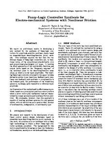
Fig. 1. Full template with one, two, and three locations

In this paper, we propose a new synthesis approach, where the size and general shape of the controller is fixed in advance in the form of a template. A template is a timed or untimed automaton with parametric control structure. Figures 1 and 2 show two example template families. In the full template, shown in Figure 1, every pair of locations is connected by an edge for every possible action. In the cyclic-executive template, shown in Figure 2, the controller implements some schedule according to which the actions are handled; the controller alternates between waiting for an uncontrollable action and responding with some controllable action. The template families are organized according to the number of locations. Typically, we start the synthesis process with small templates and then iteratively increase the size until an optimal controller is found. A controller matches a template if it can be obtained by removing a subset of the edges. We encode the presence of edges using Boolean parameter variables and combine the resulting parametric timed automaton with the plant automaton: any valuation of the Boolean parameters under which only safe states are reachable represents a correct controller. Template-based synthesis has several attractive features: Since the observations of the controller are limited by the template, template-based synthesis naturally solves the controller synthesis problem with partial observability. The size of the controller is also limited by the size of the template. Because the templates model standard types of controllers, the synthesized controllers are well-structured, resembling a manually built controller. In terms of complexity, it is not surprising that template-based synthesis is much simpler than standard synthesis. The problem is PSpace-complete, matching the complexity of model checking. Template-based synthesis can in fact be understood as parametric model checking, where we verify a timed automaton that is parametrized with Boolean variables. The technical challenge in developing fast algorithms for template-based synthesis thus lies in the efficient manipulation of the potential valuations of the parameters. In the paper, we present a solution to this challenge based on auto-

Template-based Controller Synthesis for Timed Systems c!

a? b? d! c!

3

a?

c!

a?

b?

d!

b?

d!

Fig. 2. Cyclic-executive template with two and four locations

matic abstraction refinement. Starting with an initial abstraction that considers all parameter valuations, a refinement loop incrementally focuses the search towards smaller and smaller sets of parameter valuations. The loop terminates as soon as, for the remaining parameter valuations, only safe states are reachable. New refinements are computed by identifying situations where an unsafe state is reachable for a subset of the parameter valuations. Our experimental results indicate that template-based synthesis is not only an effective solution to the controller synthesis problem with partial observability, it is an attractive alternative to standard synthesis also in the simpler case of complete observability, outperforming tools like Uppaal-Tiga on benchmarks where structurally simple controllers, corresponding to the available templates, exist. Related work. The basic timed controller synthesis problem for timed automata [AD94] with complete observability was defined by Maler et al. [MPS95,AMPS98] in the setting of turn-based timed games. In their fundamental work, the decidability of the problem was shown by demonstrating that the standard discrete attractor construction [Tho95] on the region graph suffices to obtain winning strategies. Henzinger and Kopke showed that this construction is theoretically optimal by proving that the problem is ExpTime-complete [HK99]. D’Souza and Madhusudan investigated the complexity of timed controller synthesis against external specifications [DM02]. Bouyer et al. continued this line of research and also investigated the impact of partial information [BDMP03]. A first more practical approach to timed controller synthesis, implemented in the tool SynthKro, was proposed by Altisen and Tripakis [AT02]. The approach requires, however, an expensive preprocessing step. Cassez et al. presented a symbolic algorithm, implemented in Uppaal-Tiga, that avoids the upfront state explosion by combining the backward attractor construction with a forward zone graph exploration [CDF+ 05,BCD+ 07]. Our timed verification and synthesis tool Synthia [PEM11] is based on abstraction refinement techniques that combine symbolic representations for the discrete and the continuous state components [EMP10] and exploit the compositional structure of the timed system [PM09]. We have implemented the approach presented in this paper as an extension of Synthia. Compared to the significant body of work on timed controller synthesis with complete observability, there has been comparatively little work on the more re-

4

Bernd Finkbeiner and Hans-J¨ org Peter

alistic setting of partial observability. Fundamental results on the undecidability of the general problem and the complexity for fixed granularity are due to Bouyer et al. [BDMP03]. Cassez et al. proposed a pragmatic approach to handle partial information, which restricts the choices and the observability of the controller so that a zone-based synthesis algorithm remains possible [CDL+ 07]. An extension of this work uses alternating timed simulation relations to efficiently control partially observable systems [CDL09]. This approach has also been implemented in Uppaal-Tiga. Template-based synthesis is related to the bounded synthesis approach [SF07], where one fixes the size (but not the structure) of the controller. Bounded synthesis has so far been limited to purely discrete systems. There are efficient algorithms for bounded synthesis based on SMT-solving [FS07], antichains [FJR09], and BDDs [Ehl10], which, however, unfortunately do not seem to have straightforward extensions to the timed case. Another interesting restriction on the type of controllers to be considered has been proposed by Lustig et al.: synthesis from component libraries [LV09] attempts to construct a controller by assembling routines from a given library. The difference to template-based synthesis is that the synthesized controller is a combination of predefined components rather than an instantiation of a parametric template. Currently, this approach is also limited to discrete systems.

2

Timed Systems

Timed automata. The components of a timed system are represented by timed automata. A timed automaton [AD94] is a tuple A = (L, l0 , Σ, ∆, X, I), where L is a finite set of (control) locations, l0 ∈ L is the initial location, Σ is a finite set of actions, ∆ ⊆ (L × Σ × C(X) × 2X × L) is an edge relation, X is a finite set of real valued clocks, I : L → C(X) maps each location to an invariant, and C(X) is the set of clock constraints over X. A (rectangular) clock constraint ϕ ∈ C(X) is of the form ϕ = true | x ≤ c | c ≤ x | x < c | c < x | ϕ1 ∧ ϕ2 ,

N

where x is a clock in X and c is a constant in 0 . A clock valuation t : X → IR≥0 assigns a nonnegative value to each clock and can also be represented by a |X|dimensional vector t ∈ R, where R = IRX ≥0 denotes the set of all clock valuations. The states of a timed automaton are pairs (l, t) of locations and clock valuations. Timed automata have two types of transitions: timed transitions, where only time passes and the location remains unchanged, and discrete transitions, where no time passes, the current location can be changed and some clocks can d be reset to zero. In a timed transition, denoted by (l, t) − → (l, t + d · 1), the same nonnegative value d ∈ IR≥0 is added to all clocks such that, for each 0 ≤ d0 ≤ d, t + d0 satisfies the location invariant I(l). A discrete transition, denoted by a (l, t) − → (l0 , t0 ) for some action a ∈ Σ, corresponds to an edge δ = hl, a, ϕ, λ, l0 i of ∆ such that t satisfies the clock constraint ϕ of δ, and t0 = t[λ := 0] is obtained

Template-based Controller Synthesis for Timed Systems

5

from t by setting the clocks in λ to 0 and satisfies the location invariant I(l0 ). δ

For two states s and s0 , we write s − → s0 if there is a delay d ∈ IR≥0 and an d

a

edge δ with action a such that there is an s00 with s − → s00 and s00 − → s0 . We say that a state s is reachable if there is a finite sequence of transitions δ

δn−1

0 s1 . . . sn−1 −−−→ s such that δ0 , . . . , δn−1 ∈ ∆ are edges in ∆, of the form s0 −→ s0 = (l0 , 0) is the initial state (where 0 is the zero vector), and for all 1 ≤ i ≤ n, the individual si = (li , ti ) are states of the automaton. We define Reach(A) as the set of all forward reachable states of a timed automaton A.

Composition. Timed automata can be composed to networks, in which the automata run in parallel and synchronize on shared actions. For two timed automata A = (L1 , l01 , Σ1 , ∆1 , X1 , I1 ) and A0 = (L2 , l02 , Σ2 , ∆2 , X2 , I2 ) with disjoint clock sets X1 ∩ X2 = ∅, the parallel composition A1 kA2 is the timed automaton (L1 × L2 , (l01 , l02 ), Σ1 ∪ Σ2 , ∆, X1 ∪ X2 , I), where I(l1 , l2 ) = I1 (l1 ) ∧ I2 (l2 ) for all l1 ∈ L1 and l2 ∈ L2 , and ∆ is the smallest set that contains – for a ∈ Σ1 ∩ Σ2 , h(l1 , l2 ), a, ϕ1 ∧ ϕ2 , λ1 ∪ λ2 , (l10 , l20 )i if hl1 , a, ϕ1 , λ1 , l10 i ∈ ∆1 and hl2 , a, ϕ2 , λ2 , l20 i ∈ ∆2 , – for a ∈ Σ1 \ Σ2 , h(l1 , l2 ), a, ϕ1 , λ1 , (l10 , l2 )i if hl1 , a, ϕ1 , λ1 , l10 i ∈ ∆1 , and – for a ∈ Σ2 \ Σ1 , h(l1 , l2 ), a, ϕ2 , λ2 , (l1 , l20 )i if hl2 , a, ϕ2 , λ2 , l20 i ∈ ∆2 . Finite Semantics. The decidability of the reachability problem of timed automata relies on the existence of the region equivalence relation [AD94] on R which has a finite index. For a timed automaton A = (L, l0 , Σ, ∆, X, I), we call the value of a clock x ∈ X maximal if it is strictly greater than the highest constant cmax any clock is compared to. We say that two clock valuations t1 , t2 ∈ R are in the same clock region, denoted t1 ∼R t2 , if – the set of clocks with maximal value is the same in t1 and in t2 (∀x ∈ X : t1 (x) > cmax ⇔ t2 (x) > cmax ), and – t1 and t2 agree (1) on the integer parts of the clock values, (2) on the relative order of the noninteger parts of the clock values, and (3) on the equality of the noninteger parts of the clock values with 0. That is, for all clocks x and y with nonmaximal value, it holds that (1) bt1 (x)c = bt2 (x)c, (2) bt1 (x) ≤ bt1 (y) ⇔ bt2 (x) ≤ bt2 (y), and (3) bt1 (x) = 0 if, and only if, bt2 (x) = 0, where bti (x) = ti (x) − bti (x)c for i ∈ {1, 2}. We denote with [t]R = {t0 ∈ R | t ∼R t0 } the clock region t belongs to. We say that two states s1 = (l1 , t1 ) and s2 = (l2 , t2 ) of A are region-equivalent, denoted by s1 ∼R s2 , if their locations are the same (l1 = l2 ) and the clock valuations are in the same clock region (t1 ∼R t2 ), and denote with [(l, t)]R = {(l, t0 ) ∈ L × R | t ∼R t0 } the equivalence class of region-equivalent states that (l, t) belongs to. Regions are a suitable semantics for the abstraction of timed automata because they essentially preserve the language: if there is a discrete transition a s− → s0 from a state s to a state s0 of a timed automaton, then there is, for all a states r with r ∼R s, a state r0 with r0 ∼R s0 such that r − → r0 is a discrete

6

Bernd Finkbeiner and Hans-J¨ org Peter

transition with the same label. For timed transitions, a slightly weaker property t holds: if there is a timed transition s → − s0 from a state s to a state s0 , then there is, for all states r with r ∼R s, a state r0 with r0 ∼R s0 such that there is a timed t0

transition r − → r0 (but possibly with t0 6= t). The finite semantics of a timed automaton A = (L, l0 , Σ, ∆, X, I) is the finite graph JAK = (Q, q0 , T ) where

– the symbolic state set Q = {[(l, t)]R | (l, t) ∈ L × R} of JAK is the set of equivalence classes of region-equivalent states of A, with – the initial state q0 = [(l0 , t0 )]R , and a – the set T = {(q, q 0 ) ∈ Q × Q | ∃r ∈ q, r0 ∈ q 0 , a ∈ Σ ∪ IR≥0 . r − → r0 } of transitions.

The finite semantics is reachability-preserving: Lemma 1. [AD94] For a timed automaton A = (L, l0 , Σ, ∆, X, I) there is a 0 0 finite path from astate (l,   t) to a state (l , t ) if, and only if, there is a finite path 0 0 from (l, t) R to (l , t ) R in JAK. Assuming a binary encoding of the constants in the clock constraints, the number of states of the finite semantics is exponential in the number of clocks and in the magnitude of the constants:

Lemma 2. [AD94] For a timed automaton A = (L, l0 , Σ, ∆, X, I), with cx as the maximal constant appearing in any constraint of A, the number of states of JAK is bounded by Y O(cx ) = |L| · |X|! · O(cx )|X| . |L| · |X|! · 2|X|−1 · x∈X

As it turns out, the finite semantics is a theoretically optimal state space representation for deciding reachability: Theorem 1. [AD94] For a timed automaton A and a set of states B, testing whether Reach(A) ∩ B = ∅ is PSpace-complete. In practice, instead of deciding Reach(A) ∩ B = ∅ based on an explicit construction of the finite semantics, tools like Synthia or Uppaal use the much coarser clock zones as the fundamental representation of clock values.

3

Template-based Controller Synthesis

In this section, we formalize controller templates and the template instantiation problem. A controller template is a tuple (T , P, Π) consisting of a timed automaton T = (L, l0 , Σ, ∆, X, I), a finite set of Boolean parameters P , and a total function Π : P → 2∆ defining which edges are enabled for a given parameter valuation, where P = P → is the set of all parameter valuations. In the following, we will assume that the timed automaton modeling the environment (or plant) is already integrated (by parallel composition) in T . As usual, we assume that the controller does neither reset plant clocks, inhibit plant actions, nor introduce timelocks.

B

Template-based Controller Synthesis for Timed Systems

7

Definition 1. For a controller template (T , P, Π) with T = (L, l0 , Σ, ∆, X, I) and a set of bad states B, the instantiation problem asks for a parameter valuation p ∈ P such that I = (L, l0 , Σ, Π(p), X, I) and Reach(I) ∩ B = ∅. We call an instantiation of the template that satisfies the condition of the definition feasible. Synthesizing a template-based controller corresponds to statically finding a feasible instantiation. This is in contrast to the classical formulation of the timed controller synthesis problem [MPS95,AMPS98], where the controller is an arbitrary timed automaton whose behavior depends dynamically on the observed events of the plant. The complexity of the template instantiation problem is the same as the complexity of standard timed model checking: the exponential size of the region graph dominates the size of the search space (the possible valuations of the parameters). Theorem 2. The instantiation problem for a controller template (T , P, Π) and a set of bad states B is PSpace-complete. We note that the synthesis of controllers with full observability is already ExpTime-complete [HK99]. The case where the controller can only observe a subset of the events of the plant, is even undecidable in general, or 2ExpTimecomplete if the granularity (number and precision of the clocks) of the controller is bounded in advance [BDMP03]. Furthermore, the size of the controller can be exponential or even, in case of partial observability, doubly-exponential in the size of the plant. Template-based synthesis is not only much cheaper (PSpacecomplete), it also has the advantage that the size of the controller is fixed in advance. Template-based synthesis thus provides a much more promising setting for effective controller synthesis than the standard approach. The remainder of the paper is devoted to the development of an efficient template-based synthesis algorithm and an experimental evaluation.

4

Symbolic Parameter Synthesis

We now present a symbolic algorithm for finding feasible instantiations for a given controller template (T , P, Π) with T = (L, l0 , Σ, ∆, X, I) and a set of bad states B ⊆ S, where S is the set of states of T . In the rest of this section, we assume that T , P , Π, S, and B are fixed. We develop the algorithm in three steps: first, we describe the immediate, exact, computation of the set of feasible instantiations based on forward and backward propagation; then we give an approximate computation based on an abstraction of the template; finally, we describe an abstraction refinement procedure, which increases the precision of the approximate computation until either a feasible instantiation has been found, or it has been shown that no feasible instantiation exists.

8

Bernd Finkbeiner and Hans-J¨ org Peter

4.1

Precise Computation of the Feasible Instantiations

The precise set of feasible instantiations can be computed in a standard fixed point construction that either starts from the initial state and propagates, in a forward manner, the reachable combinations of states and parameter valuations, or starts with the bad states and propagates, in a backward manner, those combinations of states and parameter valuations that have a path to the bad states. To accommodate both directions, we define a successor and a predecessor propagation function Succ, Pred : 2S×P → 2S×P with  δ Succ(Y ) = (s0 , p) ∈ S × P | ∃δ ∈ Π(p) : ∃s ∈ S : (s, p) ∈ Y ∧ s − → s0 and  δ Pred(Y 0 ) = (s, p) ∈ S × P | ∃δ ∈ Π(p) : ∃s0 ∈ S : (s0 , p) ∈ Y 0 ∧ s − → s0 . The set FR of forward-reachable states and parameter valuations and the set BR of backward-reachable states and parameter valuations are obtained by the following fixed point computations (the index identifies the round of the fixpoint iteration): FR0 = {(l0 , 0)} × P FRi+1 = Succ(FRi ) ∪ FRi FR = limi FRi

BR0 = B × P BRi+1 = Pred(BRi ) ∪ BRi BR = limi BRi .

Clearly, if there is some (s, p) ∈ FRi then this means that state s is reached after i ∈ forward steps for parameter valuation p, which corresponds to a δ1 δ2 δi path s0 −→ s1 −→ . . . −→ s, where each δ1 , δ2 , . . . , δi is in Π(p). Dually, if there is some state (s, p) ∈ BRi then this means that state s is reached after i∈ backward steps for parameter valuation p, which corresponds to a path δ1 δ2 δi s −→ s1 −→ . . . −→ b, where b ∈ B and each δ1 , δ2 , . . . , δi is in Π(p).

N

N

We can obtain the feasible instantiations either by looking for parameter valuations in FR that are not paired up with bad states, or by looking for parameter valuations in BR that are not paired up with the initial state. Both constructions identify the same set of feasible instantiations. Theorem 3. The set G = {p ∈ P | (B × {p}) ∩ FR = ∅} = {p ∈ P | ((l0 , 0), p) 6∈ BR} consists of exactly the feasible instantiations. In practice, neither construction performs well. The problem is that it is difficult and expensive to maintain the correlation between parameter valuations and reachable states; typically, each parameter valuation results in a different set of states. Instead of directly computing the precise set of parameter valuations, in the next subsection, we will present an abstraction technique that allows us to reason about approximations of parameter valuations.

Template-based Controller Synthesis for Timed Systems

4.2

9

The Focus Abstraction

We now consider an abstraction of the template based on a given set P ⊆ P of parameter valuations, which we call focus. We use the parameter valuations in P to obtain an over- or underapproximation of the sets FR and BR, by considering P as an equivalence class: we require that a transition must exist for some or all parameter valuations in P , respectively. In the following, we use an overapproximation for the forward construction and an underapproximation for the backward construction; obviously, all constructions can also be dualized. We obtain the following approximate successor and predecessor functions: P Succ , PredP : 2S → 2S with  P δ Succ (Y ) = s0 ∈ S | ∃p ∈ P : ∃δ ∈ Π(p) : ∃s ∈ Y : s − → s0 and  δ → s0 . PredP (Y 0 ) = s ∈ S | ∀p ∈ P : ∃δ ∈ Π(p) : ∃s0 ∈ Y 0 : s − Replacing the precise Succ and Pred operators in the fixed point construction from Subsection 4.1, we obtain two new fixed point constructions for the P approximations FR and BRP : P

BRP =B 0 P P BRi+1 = PredP (BRP i ) ∪ BRi BRP = limi BRP i .

FR0 = {(l0 , 0)} P P P P FRi+1 = Succ (FRi ) ∪ FRi P P FR = limi FRi P

Clearly, if there is some state s ∈ FRi then this means that state s is reached after i ∈ forward steps for a set of parameter valuations P , which corresponds δ1 δ2 δi to a path s0 −→ s1 −→ . . . −→ s, where, for each δi , there is a pi ∈ P such that δi in Π(pi ). Dually, if there is some state s ∈ BRP i then this means that state s is reached after i ∈ backward steps for a set of parameter valuations P , which δ1 δ2 δi corresponds to a path s −→ s1 −→ . . . −→ b, where b ∈ B and, for each δi and each p ∈ P , we have δi in Π(p). The following lemma clarifies the relationships between the approximate and P precise versions of FR and BR: FR overapproximates FR on P , BRP underapproximates BR on P .

N

N

Lemma 3. For every set P ⊆ P of parameter valuations, it holds that P

FR ⊇ {s ∈ S | ∃p ∈ P : (s, p) ∈ FR} and BRP ⊆ {s ∈ S | ∃p ∈ P : (s, p) ∈ BR}. Combining Lemma 3 with Theorem 3, we obtain that the focus abstraction allows us to approximate the set of feasible instantiations: A set of parameter valuations P definitely represents feasible instantiations if no bad states appear P in FR . Dually, the parameter valuations in P definitely represent infeasible instantiations if the initial state appears in BRP . Hence, we obtain the following lower and upper bounds for the set of feasible instantiations.

10

Bernd Finkbeiner and Hans-J¨ org Peter

Theorem 4. Let G be the precise set of feasible instantiations. For every set P ⊆ P, it holds that   P p ∈ P | B ∩ FR = ∅ ⊆ G ⊆ p ∈ P | p ∈ P ⇒ (l0 , 0) 6∈ BRP . In the next subsection, we will describe an automatic refinement algorithm for the Focus abstraction. 4.3

Abstraction Refinement

We now describe a refinement procedure that computes an increasingly precise approximation of the set of feasible instantiations. The procedure starts with the set P of all parameter valuations, and then splits the set into smaller and smaller subsets, until either a feasible instance is found, or it is established that no feasible instance exists. Algorithm 1 Solve(P ): The algorithm computes a safe subset of a given set P of parameter valuations, or returns fail if no safe subset exists. 1: 2: 3: 4: 5: 6: 7: 8: 9: 10: 11: 12: 13: 14:

if P = ∅ then return fail else if (l0 , 0) ∈ BRP then return fail P else if FR ∩ BRP = ∅ then return P else P1 := Refine(P ) R1 := Solve(P1 ) if R1 6= fail then return R1 else P2 := P \ P1 return Solve(P2 )

The procedure is shown as Algorithm 1. The input to the procedure is the current focus P , for which we initially use P. Unless the (un)reachability of some bad state can be surely established, after each refinement step, Solve recurs on the refined focus. In each call of Solve, the set of bad states are augmented with the states in BRP . This is justified by the following lemmas, which state that the 0 old underapproximation BRP is a subset of the new underapproximation BRP P for a refinement P 0 ⊂ P , and that excluding BRP from FR does not affect the resulting upper bound on the feasible instantiations. Lemma 4. For two sets P, P 0 ⊆ P of parameter valuations such that P 0 ⊂ P , 0 it holds that BRP ⊆ BRP . Lemma 5. For every set P ⊆ P of parameter valuations, it holds that   P P p ∈ P | B ∩ FR = ∅ = p ∈ P | BRP ∩ FR = ∅ .

Template-based Controller Synthesis for Timed Systems

11

It remains to specify the function Refine, which is called in procedure Solve to find an appropriate subset of P to split on. Since P is finite, we could, in principle, choose any strict (and non-empty) subset of P during the refinement step. In the following we describe a heuristic choice that has proved useful in practice: we choose a set of parameter valuations that are guaranteed to increase BRP in the next iteration. Suppose the termination conditions of procedure Solve are not true yet, i.e., P the initial state is not in BRP and there are still states in FR ∩ BRP . We choose P a state s ∈ F R \ BRP and a state s0 ∈ BRP , such that there exists a transition δ ∈ Π(p) that leads from s to s0 for some p ∈ P , but not for all p ∈ P . The refinement proceeds with the parameter valuations that allow a transition from s to s0 : δ

Refine(P ) = {p ∈ P | ∃δ ∈ Π(p) : s − → s0 } Since such a pair s, s0 of states can be found until the termination conditions of procedure Solve become true, we obtain that Refine always ensures progress of our refinement algorithm. Lemma 6. For every set of parameter valuations P ⊆ P, if P 6= ∅, (l0 , 0) 6∈ P P BRP , and FR ∩ BRP 6= ∅, then there is a state s ∈ FR \ BRP and a state s0 ∈ BRP such that ∅ ⊂ Refine(P ) ⊂ P. Putting everything together, we obtain the following correctness theorem for Solve(P), where Lemma 6 guarantees termination and Theorem 4 guarantees soundness of the result. Theorem 5. Called with the set P of parameter valuations, Procedure Solve(P) terminates after at most |P| refinement steps and either computes a feasible template instantiation or reports failure, in which case no feasible template instantiation exists.

5

Experimental Results

In this section, we report on experimental results based on a prototype implementation of the symbolic instantiation algorithm from Section 4. Implementation. We have implemented the symbolic instantiation algorithm from Section 4 in the Synthia tool [PEM11]. Synthia is a verification and synthesis tool for timed automata extended with bounded integer variables. The tool provides facilities for automatic abstraction refinement and combines reduced ordered binary decision diagrams (ROBDDs) [Bry86] with difference bound matrices (DBMs) [Dil89] to obtain symbolic state representations for both discrete and continuous state components.

12

Bernd Finkbeiner and Hans-J¨ org Peter

While standard Synthia already includes a game-based synthesis algorithm for timed controllers with complete observability, we only use the verification functionality of Synthia for template-based synthesis. For a template instantiation problem given by a controller template (T , P, Π) and a set of bad states, we encode the Boolean parameters P by global integer variables whose initial values are left undefined. The algorithm from Section 4 is realized as a specialized refinement procedure for Synthia’s standard (location-based) abstraction refinement loop. Whenever an edge for refinement is found, we identify the parameter valuations associated with that edge and split the global abstraction with these valuations. In the subsequent refinement step, we focus (i.e., we restrict the forward exploration) on the identified parameters of the last refinement. Benchmarks. In the Chinese Juggler benchmark [LBS], a performer needs to stabilize spinning plates to prevent them from falling. After a certain amount of time has passed since a plate was stabilized, it can nondeterministically become unstable. If no restabilization takes place, it ultimately falls down. The plates have different sizes, and hence, different times to become unstable. It takes the performer one time unit to stabilize a certain plate. During that time, he cannot stabilize another plate. The controller synthesis task consists in finding a safe strategy for the performer such that no plate will ever fall down. The benchmark size is parametrized in the number of plates n. For the template-based synthesis, we use a generic cyclic-executive template (cf. Section 1) with n locations. In each step of the cyclic execution, the controller decides which plate should be stabilized next. In the Dam benchmark, a controller is to be synthesized that determines the speed of the inflow to a dam. The controller can either stop the inflow or choose between a slow or a fast inflow speed. The bounded reachability requirement is that the fill level should reach a certain value between a minimal and maximal bound. While a fast speed might reach the desired fill level more quickly, the variance of the actual inflow is larger so that the maximal level might be exceeded. On the other hand, being in slow mode, it takes longer to reach the desired fill level, but the variance is not so high so that it is always possible to exactly reach a desired fill level. Thus, being in one mode all the time is not feasible, since a feasible controller must alternate between fast and slow at least once to fulfill the requirement. The benchmark size is parametrized in the degree of precision in which the fill level and the inflow amount is digitized. For the template-based synthesis, we use a controller template that models a parametric two-phase program: in the first phase, a certain inflow speed is set until a threshold of the current fill level is passed. Then, the controller enters the second phase with a possibly different speed. The controller stops as soon as a desired fill level is reached. The first and the second speed, as well as the phase-switching threshold are parameters, for which feasible instantiations are to be found. Results. We compare the performance of the template-based extension of Synthia against standard Synthia and Uppaal-Tiga 0.16 [BCD+ 07]. In Table 1,

Template-based Controller Synthesis for Timed Systems

13

Table 1. Experimental evaluation of template-based synthesis. We compare the performance of the template-based extension of Synthia against standard Synthia and Uppaal-Tiga.

Benchmark Juggler 2 Juggler 3 Juggler 4 Juggler 5 Juggler 6 Juggler 7 Dam 5 Dam 25 Dam 50 Dam 75 Dam 100 Dam 125 Dam 150 Dam 175 Dam 200

Template-based Synthia Standard Synthia Uppaal-Tiga Steps Abs Time Mem Steps Abs Time Mem States Time Mem 6 19 0 53 2 5 1 53 57 0 6 38 136 0 61 6 9 1 61 477 0 6 110 421 2 87 TIMEOUT 6755 6 57 423 1899 59 247 TIMEOUT 81292 1095 79 1445 8335 1932 1335 TIMEOUT TIMEOUT TIMEOUT TIMEOUT TIMEOUT 58 100 1 80 230 149 4 80 88592 2 65 268 380 13 87 1115 718 1182 91 3114648 307 443 530 730 87 105 TIMEOUT 13545848 5018 2355 793 1080 329 111 TIMEOUT TIMEOUT 1055 1430 927 143 TIMEOUT TIMEOUT 1318 1780 1949 149 TIMEOUT TIMEOUT 1580 2130 3483 153 TIMEOUT TIMEOUT 1843 2480 5127 213 TIMEOUT TIMEOUT TIMEOUT TIMEOUT TIMEOUT

the columns show, from left to right, the benchmark instance, the number of refinement steps and abstract locations in the final abstraction of the parameter synthesis algorithm, the running time and memory consumption of our templatebased implementation, the performance of Synthia’s standard controller synthesis algorithm, Uppaal-Tiga’s number of explored states, running time and memory consumption. For Uppaal-Tiga, we measured the performance for various parameters and always selected the best results. Running times are given in seconds, memory consumption in MB, the time limit was set to 2 hours, and the memory limit was set to 4 GB. All experiments were conducted on a 2.6 GHz AMD Opteron computer running Ubuntu 10.04. For both benchmarks, template-based Synthia clearly outperforms the game-based synthesis techniques implemented in standard Synthia and Uppaal-Tiga. A closer look at the Chinese Juggler example reveals that a major source of complexity results from the subtraction operation that occurs in the backwards computation of the winning states. Subtraction is expensive because it does not preserve convexity, and therefore requires a split into multiple zones. The much better performance of template-based synthesis is due to the fact that template-based synthesis is based on model checking, rather than game solving, and model checking does not require such nonconvex operations. In the Dam example, we observe that the size of the abstraction, and, thus, the running time, of the template-based approach increases polynomially in the size of the benchmark, while both standard Synthia and Uppaal-Tiga suffer from an exponential blow-up.

14

6

Bernd Finkbeiner and Hans-J¨ org Peter

Conclusion

Our results demonstrate that template-based synthesis is an attractive alternative to the standard game-based approach to timed synthesis. Template-based synthesis has the better worst-case complexity, is easier to implement with symbolic data structures such as DBMs, and produces nicely structured controllers with a small number of locations. In future work, we plan to expand the class of templates considered by the synthesis algorithm. Particularly interesting is the introduction of parameters in the clock constraints. Results from parametric timed model checking [AHV93] indicate that the analysis of such templates is in general undecidable. However, subclasses of parametric timed automata, such as L/U automata [HRSV01], for which the emptiness problem is decidable, are promising candidates for a more expressive and yet computationally feasible class of templates. The long-term goal is to obtain a succinct but comprehensive library of standard templates that serves as a basis for a fully automatic template-based synthesis approach. Acknowledgments. The authors would like to thank Alexandre David for pointing out the Chinese Juggler benchmark and Christoph Scholl for helpful comments on an early draft of the paper. This work was supported by the German Research Foundation (DFG) as part of the Transregional Collaborative Research Center “Automatic Verification and Analysis of Complex Systems” (SFB/TR 14 AVACS).

References AD94.

Rajeev Alur and David L. Dill, A theory of timed automata, Theoretical Computer Science 126 (1994), no. 2, 183–235. AHV93. Rajeev Alur, Thomas A. Henzinger, and Moshe Y. Vardi, Parametric realtime reasoning, STOC, 1993, pp. 592–601. AMPS98. Eugene Asarin, Oded Maler, Amir Pnueli, and Joseph Sifakis, Controller synthesis for timed automata, Proc. 5th IFAC Conference on System Structure and Control (J.-F. Lafay, ed.), Elsevier, 1998, pp. 469–474. AT02. Karine Altisen and Stavros Tripakis, Tools for controller synthesis of timed systems, 2nd Workshop on Real-Time Tools (RT-TOOLS), 2002. BCD+ 07. Gerd Behrmann, Agn`es Cougnard, Alexandre David, Emmanuel Fleury, Kim Guldstrand Larsen, and Didier Lime, UPPAAL-Tiga: Time for playing games!, Proc. 19th International Conference on Computer Aided Verification (CAV’07) (Werner Damm and Holger Hermanns, eds.), Lecture Notes in Computer Science, vol. 4590, Springer, 2007, pp. 121–125. BDMP03. Patricia Bouyer, Deepak D’Souza, P. Madhusudan, and Antoine Petit, Timed control with partial observability, CAV (Warren A. Hunt Jr. and Fabio Somenzi, eds.), Lecture Notes in Computer Science, vol. 2725, Springer, 2003, pp. 180–192. Bry86. Randal E. Bryant, Graph-based algorithms for boolean function manipulation, IEEE Trans. Computers 35 (1986), no. 8, 677–691.

Template-based Controller Synthesis for Timed Systems

15

CDF+ 05. Franck Cassez, Alexandre David, Emmanuel Fleury, Kim Guldstrand Larsen, and Didier Lime, Efficient on-the-fly algorithms for the analysis of timed games, Proc. 16th International Conference on Concurrency Theory (CONCUR’05) (Mart´ın Abadi and Luca de Alfaro, eds.), Lecture Notes in Computer Science, vol. 3653, Springer, 2005, pp. 66–80. CDL+ 07. Franck Cassez, Alexandre David, Kim Guldstrand Larsen, Didier Lime, and Jean-Fran¸cois Raskin, Timed control with observation based and stuttering invariant strategies, in Namjoshi et al. [NYHO07], pp. 192–206. CDL09. Thomas Chatain, Alexandre David, and Kim G. Larsen, Playing games with timed games, Proceedings of the 3rd IFAC Conference on Analysis and Design of Hybrid Systems (ADHS’09) (Zaragoza, Spain) (Alessandro Giua, Manuel Silva, and Janan Zaytoon, eds.), September 2009. Dil89. David L. Dill, Timing assumptions and verification of finite-state concurrent systems, Automatic Verification Methods for Finite State Systems (Joseph Sifakis, ed.), Lecture Notes in Computer Science, vol. 407, Springer, 1989, pp. 197–212. DM02. Deepak D’Souza and P. Madhusudan, Timed control synthesis for external specifications, STACS (Helmut Alt and Afonso Ferreira, eds.), Lecture Notes in Computer Science, vol. 2285, Springer, 2002, pp. 571–582. Ehl10. R¨ udiger Ehlers, Symbolic bounded synthesis, CAV (Tayssir Touili, Byron Cook, and Paul Jackson, eds.), Lecture Notes in Computer Science, vol. 6174, Springer, 2010, pp. 365–379. EMP10. R¨ udiger Ehlers, Robert Mattm¨ uller, and Hans-J¨ org Peter, Combining symbolic representations for solving timed games, FORMATS (Krishnendu Chatterjee and Thomas A. Henzinger, eds.), Lecture Notes in Computer Science, vol. 6246, Springer, 2010, pp. 107–121. FJR09. Emmanuel Filiot, Naiyong Jin, and Jean-Fran¸cois Raskin, An antichain algorithm for ltl realizability, CAV (Ahmed Bouajjani and Oded Maler, eds.), Lecture Notes in Computer Science, vol. 5643, Springer, 2009, pp. 263–277. FS07. Bernd Finkbeiner and Sven Schewe, SMT-based synthesis of distributed systems, Proceedings of the 2nd Workshop on Automated Formal Methods (AFM 2007), 6 November, Atlanta, Georgia, USA, ACM Press, 2007, pp. 69–76. HK99. Thomas A. Henzinger and Peter W. Kopke, Discrete-time control for rectangular hybrid automata, Theoretical Computer Science 221 (1999), no. 1-2, 369–392. HRSV01. Thomas Hune, Judi Romijn, Mari¨elle Stoelinga, and Frits W. Vaandrager, Linear parametric model checking of timed automata, TACAS (Tiziana Margaria and Wang Yi, eds.), Lecture Notes in Computer Science, vol. 2031, Springer, 2001, pp. 189–203. LBS. Kim G. Larsen, Gerd Behrmann, and Arne Skou, Exercises for Uppaal, http://www.cs.aau.dk/~bnielsen/TOV08/ESV04/exercises. LV09. Yoad Lustig and Moshe Y. Vardi, Synthesis from component libraries, FOSSACS (Luca de Alfaro, ed.), LNCS, vol. 5504, 2009, pp. 395–409. MPS95. Oded Maler, Amir Pnueli, and Joseph Sifakis, On the synthesis of discrete controllers for timed systems (an extended abstract), Proc. 12th Annual Symposium on Theoretical Aspects of Computer Science (STACS’95) (Ernst W. Mayr and Claude Puech, eds.), Lecture Notes in Computer Science, vol. 900, Springer, 1995, pp. 229–242.

16

Bernd Finkbeiner and Hans-J¨ org Peter

NYHO07. Kedar S. Namjoshi, Tomohiro Yoneda, Teruo Higashino, and Yoshio Okamura (eds.), Automated technology for verification and analysis, 5th international symposium, atva 2007, tokyo, japan, october 22-25, 2007, proceedings, Lecture Notes in Computer Science, vol. 4762, Springer, 2007. PEM11. Hans-J¨ org Peter, R¨ udiger Ehlers, and Robert Mattm¨ uller, Synthia: Verification and synthesis for timed automata, CAV (Ganesh Gopalakrishnan and Shaz Qadeer, eds.), Lecture Notes in Computer Science, vol. 6806, Springer, 2011, pp. 649–655. PM09. Hans-J¨ org Peter and Robert Mattm¨ uller, Component-based abstraction refinement for timed controller synthesis, IEEE Real-Time Systems Symposium (Theodore P. Baker, ed.), IEEE Computer Society, 2009, pp. 364–374. SF07. Sven Schewe and Bernd Finkbeiner, Bounded synthesis, in Namjoshi et al. [NYHO07], pp. 474–488. Tho95. Wolfgang Thomas, On the synthesis of strategies in infinite games, STACS, 1995, pp. 1–13.

Template-based Controller Synthesis for Timed Systems

A

17

Proofs

Theorem 2. The controller template instantiation problem for a controller template (T , P, Π) and a set of bad states B is PSpace-complete. Proof. We assume T = (L, l0 , Σ, ∆, X, I). PSpace-hardness follows immediately from Theorem 1 as the original reachability problem for timed automata is just a special case of the instantiation problem: choose Π in such a way that Π(p) = ∆, for any p. Membership in NPTimePSpace ⊆ NPSpace, which is known to coincide with PSpace, is established through the following nondeterministic algorithm. First, observe that the number of possible controllers is bounded by the number of distinct parameter valuations |P| = 2|P | . Hence, some controller can be represented using only |P | bits. Our algorithm now proceeds as follows. It first guesses the bits of a feasible controller instantiation I in linear time and then verifies the guess by model checking I, which, according to Theorem 1, is in PSpace. This concludes the proof of the upper bound. t u Theorem 3. The set G = {p ∈ P | B × {p} ∩ FR = ∅} = {p ∈ P | ((l0 , 0), p) 6∈ BR} consists of exactly the feasible instantiations. Proof. It is easy to see that Gf = {p ∈ P | B × {p} ∩ FR = ∅} comprises exactly those parameter valuations for which no bad state is forward reachable. Hence, by definition, G = Gf . On the other hand, because for every forward reachable state s, the initial state s0 is also backward reachable from s, we have that Gb = {p ∈ P | ((l0 , 0), p) 6∈ BR} coincides with Gf . Hence, G = Gf = Gb . t u Lemma 3. For every set P ⊆ P of parameter valuations, it holds that P

FR ⊇ {s ∈ S | ∃p ∈ P : (s, p) ∈ FR} and BRP ⊆ {s ∈ S | ∃p ∈ P : (s, p) ∈ BR}. P

Proof. We first show FR ⊇ Y = {s ∈ S | ∃p ∈ P : (s, p) ∈ FR}. By definition, for every state s contained in Y , there is a p ∈ P such that there is a path δ

δ

δ

0 1 n s0 −→ s1 −→ . . . −→ s,

where, for each 0 ≤ i ≤ n, δi ∈ Π(p). On the other hand, by definition, for every P state s contained in FR , there is a path δ

δ

δ

0 1 n s0 −→ s1 −→ . . . −→ s,

18

Bernd Finkbeiner and Hans-J¨ org Peter

where, for each δi , 0 ≤ i ≤ n, there is a pi ∈ P such that δi in Π(pi ). Now, P when we fix each pi = p, for some p ∈ P , then we get Y . Hence, FR ⊇ Y . P Secondly, we show BR ⊆ Y = {s ∈ S | ∃p ∈ P : (s, p) ∈ BR}. By definition, for every state s contained in Y , there is a b ∈ B and a p ∈ P such that there is a path δ

δ

δ

n 1 0 b, . . . −→ s1 −→ s −→

where, for each 0 ≤ i ≤ n, δi ∈ Π(p). On the other hand, by definition, for every state s contained in BRP , there is a b ∈ B such that there is a path δ

δ

δ

n 1 0 b, . . . −→ s1 −→ s −→

where, for each δi , 0 ≤ i ≤ n, and each p ∈ P , we have δi ∈ Π(p). Now, it is easy to see that every state s in BRP , is backward reachable for an arbitrary p ∈ P , and thus, also contained in Y . Hence, BRP ⊆ Y . t u Theorem 4. Let G be the precise set of feasible instantiations. For every set P ⊆ P,   P p ∈ P | B ∩ FR = ∅ ⊆ G ⊆ p ∈ P | p ∈ P ⇒ (l0 , 0) 6∈ BRP . Proof. We first show that Y =



p ∈ P | B ∩ FR

P

= ∅ ⊆ G. By Lemma 3,

P

FR overapproximates those states that are precisely forward reachable for P . P By definition of Y , either (1) Y = ∅ ⊆ G, if B ∩ FR 6= ∅, or (2) Y = P , P if B ∩ FR = ∅, i.e., surely no bad state is reachable for P . By Theorem 3, a parameter valuation is feasible if no bad state is forward reachable. Hence, also in case (2), Y = P ⊆ G.  Secondly, we prove that G ⊆ Y = p ∈ P | p ∈ P ⇒ (l0 , 0) 6∈ BRP by showing that every p ∈ G is also contained in Y . We distinguish two cases. Case 1: assume p ∈ G ∩ P . By Theorem 3, since p ∈ G, the initial state is not backward reachable for p. By Lemma 3, BRP underapproximates those states that are precisely backward reachable for P . Since p ∈ P , we have that the premise and the implicant of the definition of Y are true, and thus, p is also contained in Y . Case 2: assume p ∈ G \ P . p violates the premise in the implication of the definition of Y , and thus, is trivially contained in Y . Hence, G ⊆ Y . t u Lemma 4. For two sets P, P 0 ⊆ P of parameter valuations such that P 0 ⊂ P , 0 it holds that BRP ⊆ BRP . 0

Proof. We assume P 0 ⊂ P and prove BRP ⊆ BRP by showing that every state 0 in BRP is also contained in BRP . By definition, for every state s ∈ BRP , there is a b ∈ B such that there is a path δ

δ

δ

0 1 n s −→ s1 −→ . . . −→ b,

Template-based Controller Synthesis for Timed Systems

19

where, for each δi , 0 ≤ i ≤ n, and each p ∈ P , we have δi ∈ Π(p). Now, it is easy to see that the same path also exists for the smaller set P 0 ⊂ P . t u Lemma 5. For every set P ⊆ P of parameter valuations, it holds that 

 P P p ∈ P | B ∩ FR = ∅ = p ∈ P | BRP ∩ FR = ∅ .

  P P Proof. Let Y = p ∈ P | B ∩ FR = ∅ and Y 0 = p ∈ P | BRP ∩ FR = ∅ . We distinguish two cases: P Case 1: assume B ∩ FR 6= ∅. In this case, since B ⊆ BRP , Y = Y 0 = ∅. P Case 2: assume B ∩ FR = ∅. Observe that, for each state s ∈ BRP , there is a path from s to some state b ∈ B, for all parameter valuations in P . On the P other hand, by assumption, FR does not comprise any states leading to some P bad state for some parameter valuation in P . Hence, BRP ∩ FR = ∅, and thus, Y = Y 0. t u Lemma 6. For every set of parameter valuations P ⊆ P, if P 6= ∅, (l0 , 0) 6∈ BRP , P P and FR ∩ BRP 6= ∅, then there is a state s ∈ FR \ BRP and a state s0 ∈ BRP such that ∅ ⊂ Refine(P ) ⊂ P. P

Proof. By assumption, since FR ∩ BRP 6= ∅, there is a path from s0 = (l0 , 0) to some state b ∈ BRP of the form δ

δ

δ

0 1 n s0 −→ s1 −→ . . . sn −→ b,

where, for each δi , 0 ≤ i ≤ n, there is a pi ∈ P such that δi in Π(pi ). Since P s0 6∈ BRP , there is surely some si ∈ FR \BRP , whose successor si+1 is in BRP . In fact, if b is the first state from BRP which appears on the path, then a candidate δn edge for refinement is sn −→ b, i.e., s = sn and s0 = b. Thus, ∅ ⊂ Refine(P ) as Refine(P ) contains those p ∈ P , for which δn ∈ Π(p). On the other hand, if Refine(P ) subsumes exactly those p ∈ P , for which δn ∈ Π(p), we can conclude that Refine(P ) ⊂ P , as sn would be contained in BRP in the first place if δn would be available for all p ∈ P . t u Theorem 5. Called with the set P of parameter valuations, Procedure Solve(P) terminates after at most |P| refinement steps and either computes a feasible template instantiation or reports failure, in which case no feasible template instantiation exists. Proof. Termination of Solve(P) is easily established by applying Lemma 6 which ensures progress of each refinement step. Since there are only finitely many parameter valuations in P, the focus P will eventually, after at most |P| refinement steps, end up with ∅ or some parameter valuations for which one of the termination conditions becomes true.

20

Bernd Finkbeiner and Hans-J¨ org Peter

Soundness of Solve(P) follows immediately from Theorem 4. Completeness of Solve(P) is established by the fact that Solve does not miss any parameter valuation: in the lines 9 and 14 of Algorithm 1, Solve recurs on the refinement P1 and on P \ P1 . t u