Jun 4, 2015 - Croquette (1989) and Morris et al. (1991). Defects are imperfections in the .... mesh gets finer towards the side wall. It is obtained by a geometric ...
1
arXiv:1506.01560v1 [physics.flu-dyn] 4 Jun 2015
Large-scale mean patterns in turbulent convection Mohammad S. Emran and J¨ org Schumacher Institut f¨ ur Thermo- und Fluiddynamik, Postfach 100565, Technische Universit¨ at Ilmenau, D-98684 Ilmenau, Germany
Large-scale patterns, which are well-known from the spiral defect chaos regime of thermal convection at Rayleigh numbers Ra < 104 , continue to exist in three-dimensional numerical simulations of turbulent Rayleigh-B´enard convection in extended cylindrical cells with an aspect ratio Γ = 50 and Ra > 105 . They are uncovered when the turbulent fields are averaged in time and turbulent fluctuations are thus removed. We apply the Boussinesq closure to estimate turbulent viscosities and diffusivities, respectively. The resulting turbulent Rayleigh number Ra∗ , that describes the convection of the mean patterns, is indeed in the spiral defect chaos range. The turbulent Prandtl numbers are smaller than one with 0.2 ≤ P r∗ ≤ 0.4 for Prandtl numbers 0.7 ≤ P r ≤ 10. Finally, we demonstrate that these mean flow patterns are robust to an additional finite-amplitude side wall-forcing when the level of turbulent fluctuations in the flow is sufficiently high.
1. Introduction The formation of regular patterns close to the onset of a hydrodynamic instability in spatially extended flows is well documented for generic cases. The most prominent examples are convection rolls in Rayleigh-B´enard flow (Busse (1978), Bodenschatz et al. (2000)) heated from below and cooled from above, Taylor vortices in Taylor-Couette flow (Andereck et al. (1986)) between two rotating concentric cylinders and inclined turbulent stripe patterns in plane-shear flows driven by a pressure gradient or a wall movement (Barkley & Tuckerman (2005), Duguet & Schlatter (2013)). Specifically linearly unstable systems, such as Rayleigh-B´enard convection, with a sharp transition threshold to the convective flow state allow then for a perturbative expansion about the first unstable mode at onset. The expansion leads to an amplitude equation which is simpler than the original fluid equations and describes the formation of simple patterns as a function of the system parameters (Cross & Hohenberg (1993), Hoyle (2006)). The derivation of nonlinear phase diffusion equations allows to model increasingly complex patterns, such as spirals or defects (Hoyle (2006)), which have also been detected in experiments, e.g., by Croquette (1989) and Morris et al. (1991). Defects are imperfections in the patterns such as dislocations (Cross & Greenside (2009)). In large-aspect ratio cells, this results in a state of slowly evolving spirals and defects which is known as spiral defect chaos (SDC). In such SDC regimes, all symmetries of the governing equations have been spontaneously broken (Busse (2003)). For example, the azimuthal symmetry of the roll patterns is broken in an extended cylindrical cell. When the temperature difference across the fluid layer is further increased, the fluid motion crosses over from the weakly nonlinear to the turbulence regime. The dimensionless Rayleigh number Ra = gα∆T H 3 /(νκ) describes the thermal driving. It contains the acceleration due to gravity, g, the thermal expansion coefficient at constant pressure, α, the outer sustained temperature difference across the layer, ∆T , and the height of the layer (or convection cell), H. The kinematic viscosity of the fluid ν
2
Mohammad S. Emran and J¨ org Schumacher
and the thermal diffusivity κ of the temperature field form the second important dimensionless parameter which relates dissipation in the working fluid to thermal diffusion, the Prandtl number P r = ν/κ. Turbulence is characterized by an irregular, stochastic and three-dimensional fluid motion. Does this however imply that the patterns for velocity and temperature which are documented in the SDC regime at lower Rayleigh number disappear? If not, how can these patterns be extracted? How robust are they with respect to variations of the Prandtl number? And finally, how robust are they with respect to an additional side wall-forcing which is added to the momentum equation? These are the questions which we want to address in the present work. Our investigation is based on three-dimensional direct numerical simulations (DNS) in very large aspect ratio cells which are comparable to laboratory experiments in pattern formation (Bodenschatz et al. (2000)). We conducted a series of DNS of the Boussinesq equations in cylindrical cells with an aspect ratio of Γ = D/H = 50 with D being the diameter of the cell. Our investigation extends previous numerical studies of turbulent Rayleigh-B´enard convection by Hartlep et al. (2005), Hardenberg et al. (2008) and BailonCuba et al. (2010) to very large aspect ratios Γ (see also Chill`a & Schumacher (2012)). We show that patterns very similar to SDC continue to exist into the soft turbulence regime, up to Rayleigh numbers Ra = 500 000 which were accessible here. The patterns are covered by an increasing amplitude of velocity fluctuations and become visible only after a time averaging over a sequence of flow snapshots. We then determine turbulent viscosities, ν∗ , and diffusivities, κ∗ , for the time-averaged roll patterns and define turbulent Rayleigh and Prandtl numbers for the mean flow patterns. That means we replace gα∆T H 3 � Ra ν∗ κ∗
Ra → Ra∗ =
and
P r → P r∗ =
ν∗ ∼ O(1) . κ∗
(1.1)
These turbulent Rayleigh numbers are significantly smaller than the original ones and fall consistently back into a range that corresponds with the original spiral defect chaos regime. The turbulent Prandtl numbers decrease as well and remain smaller than one. The value of P r∗ depends weakly on P r. It increases with increasing P r.
2. Numerical model We perform DNS of the three-dimensional Boussinesq equations which are given by ∂ui ∂ui 1 ∂p ∂ 2 ui + uj =− +ν + αg(T − T0 )δ3i + fi , ∂t ∂xj ρ0 ∂xi ∂x2j ∂uj = 0, ∂xj ∂T ∂T ∂2T + uj =κ 2 , ∂t ∂xj ∂xj
(2.1) (2.2) (2.3)
where p(xk , t) is the pressure, ui (xk , t) the velocity field, ρ0 the constant mass density, and T (xk , t) the temperature field. The temperature T0 is a reference temperature. Summation is applied over index j in Eqns. (2.1) – (2.3), where i, j, k = 1, 2, 3. The last term on the right hand side of Eq. (2.1), which is denoted by fi (xk , t), stands for an additional volume forcing. It is applied close to the side walls of the convection cell and designed such that it enforces the azimuthal symmetry in the vicinity of the side walls. This additional forcing is applied for two runs only which are discussed in section 3.3. The velocity field has a no-slip boundary condition on all walls. The temperature boundary condition is isothermal at the top and bottom plates and adiabatic at the
Large-scale mean patterns in turbulent convection
Run
Nφ × Nr × Nz
1 2 2a 3 4 5
601 × 401 × 97 601 × 401 × 97 1201 × 601 × 141 601 × 401 × 97 601 × 401 × 97 601 × 401 × 97
Ra 5 000 500 000 500 000 500 000 5 000 500 000
Γ Pr 50 50 50 50 50 50
0.7 0.7 0.7 3 10 10
N u Re NBL 1.84 14 7.72 204 7.25 209 8.38 62 2.00 1 8.71 22
3
Ra∗ P r∗
30 – 10 4500 16 4800 10 7300 29 – 9 39000
– 0.21 0.21 0.38 – 0.40
Table 1. Parameters of the different simulations. The column NBL displays the number of grid points inside the thermal boundary layer. The last two columns display the turbulent Rayleigh and Prandtl numbers, respectively, analyzed for selected runs. Run 2a is conducted at a higher grid resolution as run 2.
side wall. The problem is formulated in cylindrical coordinates (r, φ, z) and solved by a second-order finite difference scheme (Verzicco & Camussi (2003)). In Table 1, we list the simulation parameters and grid resolutions for each DNS run. The azimuthal spacing (∆φ ) is uniform, the radial (∆r ) and axial (∆z ) grid sizes are nonuniform. The radial mesh gets finer towards the side wall. It is obtained by a geometric scaling relation which clusters the grid points less than Tchebychev collocation points when the side wall is approached, r → D/2. This also means that azimuthal grid spacing r∆φ grows for growing r. The grid resolution in the cylindrical cell with very large aspect ratio puts a challenge to the simulations, in particular in terms of the azimuthal resolution. Following Gr¨ otzbach (1983), we tested p our DNS grid by calculating the global maximum ˜ = max( 3 r∆φ ∆r ∆z ). The criterion states that ∆ ˜ ≤ πηK , of the geometric mean, ∆ where ηK is the Kolmogorov dissipation length (see also Emran & Schumacher (2008) ˜ K is 2.7 for run 2 in Table 1 and 1.7 for and Shishkina et al. (2010)). The ratio ∆/η comparison run 2a at a higher resolution. Turbulent heat and momentum transfer are compared in Tab. 1. All runs start with the diffusive equilibrium state which is perturbed randomly. Length scales are normalized in units of H, velocities in units of the free-fall velocity Uf = √ gα∆T H, time in units of the free-fall time Tf = H/Uf and temperatures in units of ∆T . The turbulent heat and momentum transport are measured by the Nusselt and Reynolds numbers, respectively. They are given by r √ Ra 2 ˜ N u = 1 + RaP rh˜ uz T iV,t , Re = h˜ u iV,t . (2.4) Pr i The notion h·iV,t stands for an ensemble average taken as a volume-time average in DNS case. From here on, we will omit the tilde for dimensionless quantities.
3. Results 3.1. Observations Figure 1 shows a sequence of three-dimensional streamline plots viewed from the top for P r = 0.7 and Γ = 50. Panel (a) and a magnification in (b) are for Ra = 5 000. For this Rayleigh number value almost no difference was found between an instantaneous snapshot and the time average which is taken over 100 Tf and not shown in the figure.
4
Mohammad S. Emran and J¨ org Schumacher
Figure 1. Streamlines of the velocity field (view from the top) and contours of the temperature field in a Rayleigh-B´enard convection cell. (a) Instantaneous velocity field pattern at Ra = 5 000 and (b) magnification, both taken from run 1 in table 1. (c) Corresponding temperature field in mid plane. (d,e) Instantaneous streamline plot and its magnification at Ra = 500 000. (f) Corresponding temperature field in mid plane. (g,h) Streamline plot of the time-averaged velocity field at Ra = 500 000 and magnification. (i) Corresponding time-averaged temperature field in mid plane. The time average in (g)–(i) is taken over τ = 200Tf . Panels (d)–(i) are for run 2 from table 1. All data are for P r = 0.7. The yellow boxes in panels (b) and (h) highlight defects in the patterns.
The corresponding temperature pattern is displayed in panel (c). Panel (d) of the same figure and its magnification (e) display an instantaneous streamline plot at Ra = 500 000. Both figures reflect the large amplitude of turbulent fluctuations. The fluctuating nature of the temperature field is also obvious in Fig. 1(f). The snapshots appear at a first glance almost featureless. The bottom panels (g)–(i) show the time averages, which are obtained for a duration of 200Tf , and its magnification. The temperature plots (f) and (i) recapture patterns which have been discussed in Hartlep et al. (2005) for similar Rayleigh and Prandtl numbers in rectangular slabs with Γ = 10. This holds particularly in the center of the convection cell. The magnified view of panel (g) in (h) confirms the wellknown result that the mean flow rolls end perpendicular to the side wall which underlines that the grid resolution is sufficient. The time-averaged plots (g)–(i) recapture now patterns that are similar to SDC, i.e., to those which are observed in panels (a)–(c) of the same figure for the Rayleigh number
Large-scale mean patterns in turbulent convection
5
Figure 2. (Color online) Determination of the drift between two successive mean flow patterns in order to quantify the slow variation. (a): Magnitude of the difference between two successive mean flow patterns taken at z0 = H/8 with τ = 50Tf . (b–d): Vk+1,k (z0 ) versus averaging interval k taken at three different z0 which are indicated in the legend and the same for all three panels. Data are for run 2 in table 1. (b) τ = 100Tf , (c) τ = 50Tf , (d) τ = 20Tf .
that is by two orders of magnitude smaller. A time average taken over τ has to be long enough such that the turbulent fluctuations in the velocity field are suppressed (τ � Tf ). However, if the averaging procedure proceeds over a very long time interval then these patterns will be washed out for all Rayleigh numbers discussed here. We can decompose the velocity and temperature fields into a time-averaged field and remaining turbulent fluctuations as ui (xj , t) = hui (xj )it + u0i (xj , t)
and
T (xj , t) = hT (xj )it + T 0 (xj , t) ,
(3.1)
where h·it denotes a time average. In Fig. 2, we analyze the slow drift of the large-scale flow pattern. The total integration time interval, T = M τ , is divided into M equidistant subintervals Ik with k = 0, M −1. These averaging intervals are taken from kτ to (k +1)τ with τ � Tf . Panel (a) of the figure shows the magnitude of the difference between two successive mean flow patterns taken at z0 = H/8. We see that pointwise differences get as high as 0.5Uf in this example. Panels (b)–(d) of Fig. 2 show a measure for the drift of the mean flow patterns which is defined as Vk+1,k (z0 ) = hui (z0 )iA,t∈Ik+1 − hui (z0 )iA,t∈Ik . (3.2) The notation h·iA,t stands for a plane-time average. Run 2 is advanced for 400Tf and this time interval is split into fractions of τ = 20, 50 and 100Tf , respectively. While for
6
Mohammad S. Emran and J¨ org Schumacher
Figure 3. Streamline plots of the velocity field in the Rayleigh-B´enard convection cell at Ra = 500 000 and P r = 10. A view from the top onto a quarter of the cell is displayed. Left: instantaneous streamline snapshot. Right: time-averaged streamline plot obtained for averaging over τ = 50Tf . Data are from run 5 in table 1.
τ = 100Tf the drift velocities in all three planes are of the same size, the data for the two smaller τ imply that the drift in the center plane is in parts slightly slower. For averaging times τ . 20Tf we reach the range of typical turnover times of a Lagrangian tracer within a large-scale circulation roll (Emran & Schumacher (2010)). Therefore, we do not consider smaller time intervals τ . In all three plots, we detect nearly the same magnitude of the drift velocity. This allows us to derive a time scale of the processes which is H/Vk+1,k & 103 Tf , a large time scale which is not accessible in this study. This time scale is comparable to that of a slow spanwise drift of streaky structures in plane Poiseuille flow which has been reported very recently by Kreilos et al. (2014). This estimate is also consistent with the one for a time scale of horizontal motion, Th , that should vary as Th = Γ2 Tf . Furthermore, we observe that the drift velocities for planes at z = δT , H/2 and H − δT are of same order of magnitude. This suggests that the mean flow roll pattern drifts slowly as a whole. Figure 3 repeats the analysis at P r = 10 and Ra = 500 000. Now, the streamlines of the snapshot appear much less disordered than for P r = 0.7. Consequently, the difference to the mean flow pattern is much smaller. One reason could be that the thermal diffusion is less compared to the momentum diffusion when the Prandtl number grows for a fixed Rayleigh number. This results in thermal plumes which have thinner stems and disperse less rapidly with respect to time. Thus the stirring of the fluid by plumes is less efficient. The result is in line with the decrease of the Reynolds number for growing Prandtl number as shown in Tab. 1. Our finding is also supported by Silano et al. (2010) who have observed decreasing peak velocities for increasing P r. In Fig. 4, we summarize the results of the Reynolds-decomposed velocity field (see the decomposition in Eq. (3.1)). In detail, we define q q q urms = hu2i iV,t , Urms = hhui i2t iV , vrms = hu0i 2 iV,t . (3.3) We include further runs at the same resolution which are not listed in Table 1, but in the caption. The smallest Rayleigh number was Ra = 2 000 for P r = 0.7 which is slightly larger than the linear instability threshold, Rac = 1 708. When expressed as a
Large-scale mean patterns in turbulent convection
7
Figure 4. (Color online) Root mean square values of the total velocity, the time-averaged velocity and the remaining turbulent fluctuations as a function of Rayleigh number Ra (see Eqns. (3.3)). Additional data points beside those listed in Tab. 1 are given at Ra = 2 000, 3 000, 4 000, 10 000, 20 000, 50 000 and 100 000 for the series at P r = 0.7 and Ra = 50 000 for P r = 10.
distance to the linear instability threshold this gives ε = (Ra − Rac )/Rac = 0.17. In this case, velocity fluctuations are practically absent, the flow pattern is almost steady consisting of several subdomains with stripe textures. With increasing Rayleigh number fluctuations of all three parts of the velocity field (see Eqns. (3.3)) grow up to Ra ≈ 5 000 which corresponds to ε = (Ra − Rac )/Rac = 1.93. At about this Rayleigh number, Urms reaches a local maximum and starts to decrease with increasing Rayleigh number. At Ra ≈ 10 000, the turbulent fluctuations vrms exceed Urms . At Ra ∼ 100 000, urms and vrms reach a local maximum and level off. For this Rayleigh number, the flow is already turbulent, the fluctuations vrms are by a factor of two larger than Urms . We also show three data sets for the case of P r = 10. The magnitudes of all three parts are significantly reduced which confirms our observation from Fig. 3. Up to the accessible Ra = 500 000 all three terms continue to grow suggesting that the maxima are shifted to higher Ra. 3.2. Estimate of turbulent viscosity and diffusivity The next step is to estimate the turbulent viscosities and diffusivities in the bulk of the cell and to evaluate the resulting turbulent Rayleigh and Prandtl numbers. We start with the Boussinesq ansatz for the closure which connects turbulent fluxes (or stresses) with the mean gradients (see e.g. Wilcox (2006); Shams et al. (2014)) and states that u0i u0j = −ν∗ijkl
∂ul , ∂xk
u0i T 0 = −κij ∗
∂T , ∂xj
(3.4)
where bars denote an appropriate space-time average. Our following estimate will aim at obtaining numbers ν∗ and κ∗ rather than exploring the full tensorial structure of the turbulent viscosities and diffusivities. This would go beyond the scope of this work. We will restrict the analysis to the dominant contributions only. In case of the turbulent diffusivity, we focus to the vertical transport of heat from the hot bottom plate to the cold top plate. The comparison of the three convective fluxes shows that the magnitude of the mean vertical flux is the largest. The turbulent
8
Mohammad S. Emran and J¨ org Schumacher
Figure 5. (Color online) Vertical profiles of the plane and time averaged correlations and derivatives which are required to determine the turbulent viscosity and diffusivity. Data displayed in the figure are obtained for Ra = 500 000 and P r = 0.7.
diffusivity, κ∗ , can be obtained by the following bulk average Z 1/2 Z 1/2 ∂hT (z)iA,t 0 0 dz . huz T (z)iA,t dz = −κ∗ ∂z δT δT
(3.5)
Time-plane averages are denoted by h·iA,t . Figure 5 displays the resulting profiles which enter the determination of κ∗ via (3.5). The double-headed arrow indicates the bulk region in the figure. In case of the momentum transport the determination is less straightforward. We can expect that the horizontal turbulent mixing is also important. First, we proceed however similar to the temperature field. We take the magnitude of horizontal velocity u⊥ (r, φ, z, t) = ur (r, φ, z, t)er + uφ (r, φ, z, t)eφ . This field is decomposed again into a temporal mean and remaining fluctuations. The turbulent viscosity, ν∗ is determined in a similar way as the turbulent diffusvity Z 1/2 Z 1/2 ∂hu⊥ (z)iA,t 0 0 huz u⊥ (z)iA,t dz = −ν∗ dz . (3.6) ∂z δT δT Here u0⊥ and u⊥ denote magnitudes. The resulting profiles that enter (3.5) and (3.6) are displayed in the right column of Fig. 5. In Tab. 1 we summarize the resulting turbulent Rayleigh and Prandtl numbers which result from this closure procedure. The turbulent Rayleigh numbers, Ra∗ , are reduced for all three cases. Ra∗ gets consistently smaller with decreasing Prandtl number P r since the amplitude of the turbulent fluctuations increases. We obtain P r∗ < P r for all three cases. Their magnitudes vary between 0.2 and 0.4. The turbulent Prandtl number P r∗ increases slightly with increasing P r. In case of runs 2 and 5, we then conducted a DNS with the same molecular viscosity and diffusivity as ν∗ and κ∗ , respectively. The resulting streamline pattern for run 2 is
Large-scale mean patterns in turbulent convection
Run 2 5
Ra
Pr
Ra∗
9
P r∗ b0 b1 b∗0 b∗1
500 000 0.7 4 500 0.21 15 8 18 7 500 000 10 39 000 0.38 20 1 18 1
Table 2. Betti numbers b0 and b1 for the original simulations at Ra and P r as well as b∗0 and b∗1 for the corresponding runs at Ra∗ and P r∗ . The number of the runs corresponds with Tab. 1. Temperature patterns at mid plane have been analyzed.
Figure 6. (Color online) Streamline plots of the velocity field in a Rayleigh-B´enard convection cell as a view from the top. Left: plot averaged for 200 Tf . Right: magnification of the same data. The DNS was conducted for Ra = 4 500, P r = 0.2 which corresponds with the turbulent viscosities and diffusivities that correspond to the time-averaged data in Fig. 1 (g,h).
displayed in Fig. 6. A time average over 200 Tf was applied at P r = 0.2 and Ra = 4 500. The flow structure has to be compared now with the time-averaged one from Fig. 1 (g,h) and indeed a reasonable visual agreement of both large-scale patterns is found. We determined the Betti numbers {b0 , b1 } from two-dimensional horizontal cuts of the mean temperature at z = 1/2 in both cases (Kurtuldu et al. (2011)). Betti numbers are d positive integers to characterize a d-dimensional set topologically. In detail, b0 is the number of connected filaments which is obtained by digitizing a grayscale picture at a threshold, b1 counts the number of enclosed holes in the pattern. We choose the temperature field in the mid plane. A threshold temperature T = 0.5 results in Betti number pairs which are listed in Tab. 2 for runs 2 and 5 as well as their corresponding runs at Ra∗ and P r∗ . Additionally, we estimated the average width of the rolls by counting the mean number of rolls that fit into the cell along different orientations. The values vary always around a width of 2H, but are not exactly equal. We also determined the turbulent viscosities from horizontal turbulent diffusion processes. It turns out that a simple adaption of the averaging procedure of Eqns. (3.5) and (3.6) to a radial dependence is not successful. The roll patterns cause radially oscillating profiles which result in strong cancellations for the averaged turbulent stresses and mean strain rates. If we omit the radial averaging and analyze the local Boussinesq relation
10
Mohammad S. Emran and J¨ org Schumacher
hu0r u0j (z)iφ,H−2δT ,t = −ν∗ (r)∂huj (r)iφ,H−2δT ,t /∂r for j = r, φ, z, we get indeed turbulent Prandtl numbers which are locally closer to one, but vary significantly with r. The resulting Ra∗ and P r∗ are such that the DNS yield time-dependent patterns, in particular for run 5 with Ra∗ = 39 000 and P r∗ = 0.4. We therefore repeated this “renormalization procedure” in the weakly nonlinear regime and obtain Ra∗∗ = 3000 and P r∗∗ = 0.13 for run 2 and Ra∗∗ = 1800 and P r∗∗ = 0.17 for run 5, respectively. Both runs end thus in the convection regime close to the onset. To summarize this section, all routes of analysis will in general not lead to turbulent Prandtl numbers P r∗ ≈ 1. A turbulent Prandtl number smaller than unity can be interpreted as follows: plume filaments of the temperature are coarser and diffuse faster than vortex filaments next to them. This circumstance could be connected to the fact that the width of rising and falling plumes is of the size of the thermal boundary layer thickness which is rather large for our Ra. In contrast, vorticity is frequently generated on finer scales. Vortex filaments are for example generated by locally reversed flows next to rising plumes, a consequence of incompressibility. An increase of the Rayleigh number to very large values could then increase the turbulent Prandtl number to one since the typical flow structures are getting finer and the boundary layers themselves are expected to become eventually fully turbulent. At this point, it should also be mentioned that the particular magnitudes of turbulent Prandtl numbers, P r∗ are still an open problem. For example, Spiegel (1971), Kays (1994), or Gr¨ otzbach (2011) discuss the dependence of P r∗ on the distance from walls or on the original P r. In case of homogeneous isotropic turbulence, Nakano et al. (1979) derived a value of P r∗ = 0.4 from a spectral formulation based on the classical Kolmogorov turbulence theory.
3.3. Robustness of large-scale mean flow patterns to additional side wall forcing The sensitivity of SDC patterns to side wall effects and suppressed mean flows has been discussed in Bodenschatz et al. (1991) and Chiam et al. (2003), respectively. This motivates us here, also in view to spontaneous symmetry breaking, to study their robustness with respect to an addition of a volume forcing to (2.1). The forcing is set up such that ˆi (r, z) with i = {r, z} very close to the it sustains a steady Lamb–Oseen–type vortex U side walls of the cell at (r0 = (Γ − 1)/2, z0 = 1/2). This vortex generates an azimuthally symmetric mean flow at the side wall. The circulation, Ω, and the radius of the vortex core, rL , are chosen such that no-slip boundary conditions can still be satisfied by setting this flow to zero below a certain threshold. This clearly prohibits a stronger variation of the amplitudes and thus of the strength of the additional forcing. Incompressibility of the full velocity field is sustained via the solution of the Poisson problem for the pressure in each time step. Figure 7 shows the results for the mean flow pattern. In case of P r = 0.7, the toroidal roll is clearly visible right at the side wall. A second roll next to the side walls can be established by the additional forcing term. Towards the center of the convection cell the mean pattern remains however unchanged as can be seen by a comparison with panels (g,h) of Fig. 1. The turbulent fluctuations are large enough to re-establish the mean flow pattern. This is different for P r = 10. In comparison to Fig. 3, the pattern has changed significantly. The toroidal roll pattern of the time averaged velocity is continued almost to the center of the cell. The reason for the stronger impact of the additional side wall forcing lies in the significantly lower level of turbulent fluctuations which we documented in Fig. 4.
Large-scale mean patterns in turbulent convection
11
Figure 7. Streamline plots of the velocity field in a Rayleigh-B´enard convection cell as a view from the top for Ra = 500 000 with the additional forcing fi (see also Eq. (2.1)). Left: P r = 0.7. Right: P r = 10. Both data sets have been averaged over 150Tf . We took Ω = 1 for the (non-dimensional) circulation and rL = 0.01 for the (non-dimensional) radius of the vortex core.
4. Summary We presented three-dimensional DNS of thermal convection in the soft turbulence regime to study time-averaged velocity field patterns and their dependence on the Prandtl number in very large aspect ratio convection cells. Our DNS demonstrate clearly that the SDC patterns, which are known from the weakly nonlinear regime, continue to exist in the turbulent regime. They remain thus dynamically relevant and do not simply disappear when convection turns into the turbulent regime. The patterns are revealed when the turbulent fluctuations are removed by time averaging over intervals of the order of 102 Tf , which is significantly smaller than the time scale over which the mean velocity and temperature patterns evolve. Our simulations allow us to calculate the turbulent viscosities and diffusivities as well as related turbulent Rayleigh and Prandtl numbers, Ra∗ and P r∗ . Their values fall indeed back into the range of the original SDC regime. The turbulent Prandtl numbers P r∗ vary between 0.2 and 0.4 and increase with increasing P r. Our studies showed also that the mean patterns are robust to finite-amplitude perturbations once the turbulent fluctuations in the flow are sufficiently large, i.e., once P r at a given Ra is sufficiently small. We demonstrated this by a side wall forcing that sustained an azimuthally symmetric vortex. Three future implications follow to our view: (i) it has to be investigated systematically if the mean flow patterns which are similar to SDC persist to even higher Rayleigh numbers or if the mean flow structure is changed. This would require numerical studies at high Rayleigh numbers and large aspect ratios. (ii) a more detailed analysis of the turbulent viscosities and diffusivities for larger Rayleigh numbers will provide useful input for technological and astrophysical applications in which the small-scale convective turbulence has to be modeled. This would however imply to explore systematically the tensorial nature of the turbulent viscosity which we did not analyze in the present work. (iii) our results could also provide useful input to reduce the degrees of freedom systematically and to derive some effective equations for the large-scale patterns, as done in other systems (Malecha et al. (2014)). This work is supported by the Deutsche Forschungsgemeinschaft. Part of this work
12
Mohammad S. Emran and J¨ org Schumacher
was completed while one of us (JS) stayed at the Institute of Pure and Applied Mathematics (IPAM) at the University of California Los Angeles. He thanks IPAM and the US National Science Foundation for financial support. Helpful comments by Janet Scheel and discussions with Jonathan Aurnou, Eberhard Bodenschatz, Friedrich Busse, Gregory Chini, and Keith Julien are acknowledged.
REFERENCES Andereck, C. D., Liu, S. S. & Swinney, H. L. 1986 Flow regimes in a circular Couette system with independently rotating cylinders J. Fluid Mech. 164, 155–183. Bailon-Cuba, J., Emran, M. S. & Schumacher, J. 2010 Aspect ratio dependence of heat transfer and large-scale flow in turbulent convection. J. Fluid Mech. 655, 152–173. Barkley, D. & Tuckerman, L. S. 2005 Computational study of turbulent laminar patterns in Couette flow. Phys. Rev. Lett. 94, 014502 (4 pages). Bodenschatz, E., de Bryun J. R., Ahlers G. & Cannell, D. S. 1991 Transitions between patterns in thermal convection. Phys. Rev. Lett.. 67, 3078–3081. Bodenschatz, E., Pesch, W. & Ahlers G. 2000 Recent developments in Rayleigh-B´enard convection. Annu. Rev. Fluid Mech. 32, 709–778. Busse, F. H. 1978 Nonlinear properties of thermal convection. Rep. Prog. Phys. 41, 1929–1967. Busse, F. H. 2003 The sequence-of-bifurcations approach towards understanding turbulent fluid flow. Surveys Geophys. 24, 269–288. Chiam, K.-H., Paul, M. R., Cross, M. C. & Greenside, H. S. 2003 Mean flow and spiral defect chaos in Rayleigh-B´enard convection. Phys. Rev. E 67, 056206 (13 pages). ` , F. & Schumacher, J. 2012 New perspectives in turbulent Rayleigh-B´enard convection. Chilla Eur. J. Phys. 35, 58 (25 pages). Croquette, V. 1989 Convective pattern dynamics at low Prandtl number. Part II. Contemp.. Phys. 30, 153–173. Cross, M. C. & Hohenberg, P. C. 1993 Pattern formation out of equilibrium. Rev. Mod. Phys. 65, 851–1112. Cross, M. C. & Greenside, H. S. 2009 Pattern formation and dynamics in nonequilibrium systems, Cambridge University Press. Duguet, Y. & Schlatter, P. 2013 Oblique laminar-turbulent interfaces in plane shear flows. Phys. Rev. Lett. 110, 034502 (4 pages). Emran, M. S. & Schumacher, J. 2008 Fine-scale statistics of temperature and its derivatives in convective turbulence. J. Fluid Mech. 611, 13–34. Emran, M. S. & Schumacher, J. 2010 Lagrangian tracer dynamics in a closed cylindrical turbulent convection cell. Phys. Rev. E 82, 016303 (9 pages). ¨ tzbach, G. 1983 Spatial resolution requirements for direct numerical simulation of the Gro Rayleigh-B´enard convection. J. Comput. Phys. 49, 241–269. ¨ tzbach, G. 2011 Revisiting the resolution requirements for turbulence simulations in nuGro clear heat transfer. Nucl. Eng. Design 241, 4379–4390. Hartlep, T., Tilgner, A. & Busse, F. H. 2005 Transition to turbulent convection in a fluid layer heated from below at moderate aspect ratio. J. Fluid Mech. 554, 309–322. von Hardenberg, J., Parodi, A., Passoni, G., Provenzale, A. & Spiegel, E. A. 2008 Large-scale patterns in Rayleigh-B´enard convection. Phys. Lett. A 372, 2223–2229. Hoyle, R. 2006 Pattern formation: An introduction to methods, Cambridge University Press. Kays, W. M. 1994 Turbulent Prandtl number – where are we? J. Heat Transfer 116, 284–295. Kreilos, T., Zammert, S. & Eckhardt, B. 2014 Comoving frames and symmetry-related motions in parallel shear flows. J. Fluid Mech. 751, 685–697. Kurtuldu, H., Mischaikow, K. & Schatz, M. F. 2011 Extensive scaling from computational homology and Karhunen-Lo`eve decomposition analysis of Rayleigh-B´enard convection experiments. Phys. Rev. Lett. 107, 034503 (4 pages). Malecha, Z., Chini, G. & Julien, K. 2014 A multiscale algorithm for simulating spatially– extended Langmuir circulation dynamics. J. Comp. Phys. 271, 131–150. Morris, S. W., Bodenschatz, E., Cannell, D. S. & Ahlers, G. 1991 Spiral defect chaos in large aspect ratio Rayleigh-B´enard convection. Phys. Rev. Lett. 71, 2026–2029.
Large-scale mean patterns in turbulent convection
13
Nakano, T., Fukushima, T., Unno, W. & Kondo, M. 1979 Viscosity, conductivity, and power spectra of the turbulent convection in Boussinesq fluids. Publ. Astron. Soc. Japan 31, 713–735. Shams, A., Roelofs, F., Baglietto, E., Lardeau, S. & Kenjeres, S. 2014 Boundary layer structure in turbulent thermal convection and its consequences for the required numerical resolution. Int. J. Heat Mass Transfer 79, 589–601. Shishkina, O., Stevens, R. A. J. M., Grossmann, S. & Lohse, D. 2010 Boundary layer structure in turbulent thermal convection and its consequences for the required numerical resolution. New J. Phys. 12, 075022 (17 pages). Silano, G, Sreenivasan, K. R. & Verzicco, R. 2010 Numerical simulations of RayleighB´enard convection for Prandtl numbers between 10−1 and 104 and Rayleigh numbers between 105 and 109 . J. Fluid Mech. 662, 409–446. Spiegel, E. A. 1971 Convection in stars: I. Basic Boussinesq convection. Annu. Rev. Astron. Astrophys. 9, 323–352. Verzicco, R. & Camussi, R. 2003 Numerical experiments on strongly turbulent thermal convection in a slender cylindrical cell. J. Fluid Mech. 477, 19–49. Wilcox, D. C. 2006 Turbulence modeling for CFD, DCW Industries.