PHYSICAL REVIEW E
VOLUME 57, NUMBER 5
MAY 1998
Spatial structure of the thermal boundary layer in turbulent convection Siu-Lung Lui and Ke-Qing Xia* Department of Physics, The Chinese University of Hong Kong, Shatin, Hong Kong, China ~Received 5 August 1997! ¯ (z) and the thermal layer thickness d (x,y) at various We have measured the mean temperature profiles T th horizontal positions on the lower plate of a cylindrical convection cell, using water as the working fluid. The Rayleigh number Ra in the experiment varied from 23108 to 231010. The normalized vertical temperature profiles measured at various positions x along the direction of large scale circulation and for the same Ra are found to be self-similar, once the vertical distance z is scaled by the respective thermal layer thickness d th(x,0). Whereas those measured at different Ra do not have a universal form. Our results further reveal that the thermal layer thickness d th varied significantly in the two directions measured—along the large-scale circulation (x) and perpendicular to it (y). We found that the scaling exponent of d th with Ra is a function of x ~and possibly a function of y as well!, i.e. d th; Ra 2 b ( x ) . Moreover, our results suggest that the thermal layer will eventually become uniform at very high Rayleigh numbers. @S1063-651X~98!02405-2# PACS number~s!: 47.27.Te, 44.25.1f.
I. INTRODUCTION
The Rayleigh-Be´nard system refers to a fluid layer confined between two horizontally parallel conducting surfaces and an insulating sidewall. Turbulent convection of the fluid occurs when the temperature difference between the two horizontal plates exceeds a certain critical value. Convective thermal turbulence is interesting both for its obvious engineering and geophysical applications and as a model system for turbulence study. When the Rayleigh number ~the dimensionless ratio of the driving energy to the dissipation one! is above ;43107 , the so-called hard turbulence regime sets in @1#. This scaling state of convective thermal turbulence is characterized @2,3# by a large-scale mean circulating flow that spans the entire system, an exponential probability distribution function of the temperature fluctuation at the center of the convection cell, and scaling laws for the heat flux and other measured quantities with exponents being different from those predicted by the ‘‘classical’’ theories @4,5#. Since the discovery of the hard turbulence regime in 1987 by Heslot, Castaing, and Libchaber @1#, much interest, both experimental and theoretical, has been focused on the study of turbulent convection @6#, and much progress has been made @2,7–13#. Although some of the proposed theoretical models @2,7# have been able to explain the observed scaling and statistical properties of the temperature field in the hard turbulence state successfully, not all of the assumptions and predictions of these models are consistent with results from later experiments @14,15#, our recent results on the scaling laws of the viscous boundary layer also provide further experimental evidence of this @16,17#. Boundary layers have long been recognized as playing a key role in convective turbulence, since the early days in the study of turbulent convectionu @18–20#. Two boundary layers exist in thermal turbulence, one viscous layer and one thermal layer; both are produced by the shear of the largescale mean circulating flow. Because heat is transported via
*Electronic address:
[email protected] 1063-651X/98/57~5!/5494~10!/$15.00
57
conduction within the thermal boundary layer, the global heat transport is intimately related to its thickness. An important assumption made in a model by Shraiman and Siggia was that the thermal layer is buried entirely within the viscous layer for large to moderate Prandtl numbers, and the reverse is true for small Prandtl numbers @7#. This assumption has been confirmed experimentally by a direct measurement of both boundary layers in water ~Pr .7) @10#, and in mercury ~Pr .0.024) where the viscous layer was indirectly measured @21#. However, most of the boundary layer measurements made so far were conducted along the central axis of a convection cell @10,16#. A question naturally arises as to whether the boundary layers are uniform across the horizontal conducting plates on which they reside. The existence of possible spatial nonuniformity of the boundary layers was first suggested by the numerical results of Werne @22# in his two-dimensional ~2D! simulation study of the hard turbulence regime. Belmonte, Tilgner, and Libchaber @14# also pointed out that in order to take into account the heat transported by thermal objects like plumes, the shear produced by the large scale circulation near the boundary should have a dependence on horizontal positions and the need to check experimentally the horizontal dependence of both viscous and thermal boundary layer properties. In her recent theoretical analysis of heat transport in the boundary layers, Ching @15# assumed horizontal dependence for both the shear rate and the thermal boundary layer thickness, and obtained a scaling relation between the heat flux and the shear rate which is in better agreement with corresponding experimental results @16,17# than a previous model @7#. Thus an experimental investigation of the boundary layers in off-centralaxis horizontal positions will not only provide information about their spatial structures, but will also serve to test some of the assumptions in, and predictions of, the abovementioned numerical and theoretical studies. In this paper, we report an experimental study of the thermal boundary layer measured at various positions on the lower plate of a cylindrical convection cell. The range of Rayleigh number ~Ra! spanned in the experiment was from 23108 to 231010. Spatial variations of the thermal layer 5494
© 1998 The American Physical Society
57
SPATIAL STRUCTURE OF THE THERMAL BOUNDARY . . .
FIG. 1. Schematic diagram of the convection cell with the movable thermistor probe for local temperature measurements. The four ‘‘black dots’’ inside the top and bottom plates are imbedded thermistors for measuring temperatures in the respective plates.
thickness were measured along two orientations, one in the direction of the large-scale circulation ~LSC! and the other one perpendicular to it. We analyze both the Ra and position dependences of the measured thermal layer, and its relation with the LSC. The rest of the paper is organized as follows. In Sec. II, we give detailed descriptions of our convection cell and the thermistor probe used for local temperature measurements. The experimental results are presented and analyzed in Sec. III, which is divided into three parts. Section III A discusses the scaling properties of the measured temperature profiles, and Secs. III B and III C discuss the positional variation and the Rayleigh number dependence of the thermal layer thickness along and perpendicular to the LSC direction, respectively. We summarize our findings and conclude in Sec. IV. II. EXPERIMENT
Figure 1 shows a schematic drawing of the convection cell, which is a vertical cylinder with its inner diameter and height being 19 and 19.6 cm, respectively ~the aspect ratio is thus near unity!. The upper and lower plates were made of copper, and their surfaces were gold plated. The sidewall of the cell was a cylindrical tube made of transparent Plexiglas. The temperature of the upper plate was regulated by passing cold water through a cooling chamber fitted on the top of the plate. The lower plate was heated uniformly at a constant rate with an imbedded film heater. The temperature difference DT between the two plates was measured by four thermistors imbedded inside the plates. The two thermistors at the top plate were at about a one-third radius from the edge at opposite positions, while the two at the bottom plate were placed at the center and the half-radius position. The measured relative temperature difference between the two thermistors in the same plate was found to be less than 1% for both plates at all Ra. This indicates that temperature was
5495
uniform across the horizontal plates. The control parameter in the experiment is the Rayleigh number Ra5 a gL 3 DT/ n k , with g being the gravitational acceleration, L the height of the cell, and a , n , and k , respectively the thermal expansion coefficient, the kinematic viscosity, and the thermal diffusivity of water, which was used as the convecting fluid. During our experiment, the average temperature of water in the convection cell was kept near room temperature, and only the temperature difference across the cell was changed. In this way, the variation of the Prandtl number Pr5 n / k was kept at minimum ~Pr.7). The thermistor used in the local temperature measurements had a diameter of 300 m m and an in-water thermal time constant of 10 ms ~AB6E3-B10KA103J, Thermometrics!. In order to access different positions in the convection cell, we used a specially designed temperature probe. As is shown in Fig. 1, a rectangular shaped stainless steel rod was soldered perpendicularly on a stainless steel capillary tubing of outer diameter 1.5 mm and inner diameter 1 mm. The horizontal rod had a cross section of 2.2 mm in height and 0.75 mm in width. A Plexiglas cube ~4 mm in side! can slide freely on the rod. The rod is marked at every 5-mm interval to indicate the exact position of the cube. The thermistor is attached at the end of a syringe needle ~outer diameter 0.5 mm, length 88 mm! which was fixed to the cube. To move the needle horizontally, two fishing strings of diameter 0.2 mm are tied to the Plexiglas cube. By pulling the two strings separately, one can move the needle in either direction along the rod to the desired horizontal position. The leads of the thermistor were fed through the needle, and then, together with the fishing strings, through the tubing to the outside. The tubing was fixed on a vertical translation stage which was mounted right above the filling stem of the convection cell. The stage has a total travel distance of 10 cm and a precision of 0.01 mm, and was driven by a computercontrolled stepper motor. In the automated temperature profile measurement along the vertical direction, a 30-min time series was first recorded by a 7 12 -digit multimeter ~Keithly 2001! at each position. The mean value and the standard deviation ~rms fluctuation! of the local temperature were then obtained from the measured resistance using a calibrated conversion curve. A typical temperature profile consists of 30 vertical positions. After completing one profile measurement, the thermistor was moved to a different horizontal position and the measurement was repeated. We measured the horizontal variation of the thermal boundary layer in directions both along the largescale circulation and perpendicular to it. To determine the direction of the LSC, we employed the following method. After the convective motion is fully established, a stainless steel tube with a very light string attached to its end is inserted into the convection cell; near the lower plate of the cell, the flow is unidirectional, so the string follows the flow and indicates its direction. It has been found by us @23# and also by others @24#, that, once established, the direction of LSC will remain the same for different Rayleigh numbers. III. RESULTS AND DISCUSSION
For ease of presentation and discussion, we first define the coordinate system for the experiment. Let the center of the
5496
SIU-LUNG AND KE-QING XIA
FIG. 2. The mean temperature ^ T & ~subtracted from the bottom plate temperature T bot and normalized by the temperature difference DT across the cell! ~circles! and the rms temperature fluctuation s ~dots! vs the vertical distance z from the bottom plate. The inset shows an enlarged region near the plate. The measurement was made at the horizontal position x58.5 cm and y50, and at Ra 51.5831010.
lower plate of the convection cell be the origin of our righthand Cartesian coordinates with the z axis pointing upward and the large-scale circulation flowing along the x axis from 2x to 1x, the y axis then being perpendicular to the LSC. Below, we discuss first the general features of the measured temperature profiles, and then examine the variations of the thermal boundary layer thickness along and perpendicular to the LSC direction, respectively. A. Scaling property of the temperature profiles
Systematic measurements were made at 11 positions on the x and the y axes, respectively. They were x528.5, 26.5, 24.5, 22.5, and 20.8 cm ~hereafter referred to as the ‘‘upstream’’ positions!, and x50.8, 2.5, 4.5, 6.5, and 8.5 cm ~hereafter called the ‘‘downstream’’ positions! on the x axis. Also, y560.8, 62.5, 64.5, 66.5, and 68.5 cm on the y axis, and at the central axis of the cell (x,y50,0). Figure 2 shows the results from a typical profile measurement at the position x58.5 cm, y50 and at Ra 51.5831010, where both the mean temperature ^ T & ~open circles! and the rms of temperature fluctuation s 5 ^ (T2 ^ T & ) 2 & 1/2 ~solid circles! are plotted as a function of the vertical distance z from the lower plate. In the figure, the mean temperature is subtracted from that of the bottom plate T bot , and then normalized by the temperature difference DT across the cell. The inset shows an enlargement of the region near the plate, where the thickness d th of the thermal boundary layer is defined as the distance at which the extrapolations of the linear part and the horizontal part of the mean temperature profile intersect. It is seen from the figure that the mean temperature profile consists of a linear portion near the plate ~where heat is mainly transported by conduction!, a ‘‘horizontal’’ portion away from the plate ~zero mean temperature gradient, which
57
FIG. 3. Scaled temperature profiles measured at various positions x along the direction of LSC at Ra 57.193109 . Here the mean temperature ~subtracted from that of the bottom plate! is normalized by the temperature scale DT, and the vertical distance z is scaled by the respective thermal layer thickness d th(x,0).
means convection dominates!, and a transitional region in between. The rms profile has a sharp maximum near d th , and then decays toward the cell center. These same features are also found for profiles measured at other horizontal positions, and are similar to those measured by others along the central axis @11#. Note also from the figure that the normalized mean temperature profile saturates at 0.5, indicating that the temperature drops at the top and bottom plates each contribute half to the total temperature difference across the cell. This implies that the Boussinesq condition @25–27# is satisfied in our system @28#. Using encapsulated liquid crystals as thermal imaging particles in water, Gluckman, Willaime, and Gollub @29# found that the temperature in the upper half of a near-cubic cell tends to be warmer than the average temperature of the cell, and that in the lower half it is cooler than the average. Tilgner, Belmonte, and Libchaber @10#, in a direct temperature profile measurement in a cubic cell in water, also found this inversion of mean temperature along the cell height ~though the deviation is only about 0.5%). Within the experimental uncertainty of our measurement, we do not see such an inversion in our cylindrical cell. Without knowing the exact circumstances of their measurements, we can only speculate that the reason is perhaps due to the geometrical shape of the cells used in the different experiments. It is known that flow patterns depend strongly on the shape of the cell, and that sharp corners in a cubic cell can produce backflows. With the change in flow field, the temperature distribution will be affected, which may result in an inversion. We found that the mean temperature profiles measured at different x all reach the same 0.5 ‘‘plateau’’ value in the center region, while their linear parts have different slopes, implying that d th changes with x. When the vertical distance z is scaled by the thickness d th(x,0), it is found that temperature profiles measured at different x but the same Ra all collapse onto a single curve, and this is true for all Ra. Figure 3 shows an example of such a scaled temperature profile for Ra57.193109 ; note from the figure that data for both the upstream (x,0) and the downstream (x.0) positions
57
SPATIAL STRUCTURE OF THE THERMAL BOUNDARY . . .
FIG. 4. Scaled temperature profiles measured along the central axis (x5y50) of the cell, and at various Ra. In the figure, the vertical and horizontal axes are normalized the same way as those in Fig. 3.
collapse together with those for the central axis (x50) almost perfectly. In his 2D numerical simulation of hard turbulence, Werne @22# found that the temperature profile is self-similar when z/ d th(x,0),1, in the sense that profiles for different x and Ra can be scaled into a single curve. A simple scaling of temperature profiles with d th(x,0) has also been assumed in a recent theoretical study @15#. Thus our results have verified the assumption of Ref. @15#, and in partial agreement with the results of Ref. @22#. But there are a few important differences between our profiles and those from the numerical study. First, our scaled profiles collapse for the entire range of z ~i.e., all the way to the cell center z5L/2), not just within the thermal layer ~in order to show the boundary layer region more clearly, only data points with z/ d th 43109 , the profiles were all reproducible, like the one shown in Fig. 5~d!. This implies that the spatial structure of thermal boundary layers was fully established only for Ra>43109 . We attribute this evolution of d th(x,0) with Ra to the gradual strengthening of the LSC. The argument here is that as the LSC is fully established, the ‘‘downhill’’ and ‘‘uphill’’ sides of the flow will become more symmetric. Since the LSC modifies the boundary layers via its shear, a symmetric LSC will give rise to a symmetric thermal layer profile. The above argument is also in line with that of Belmonte and Libchaber @33#. By finding a transition of a length scale ~associated with the power spectrum of temperature fluctuations near the boundary layer! at Ra;23109 , these authors argued that there is a turbulent transition of the large scale circulation at Ra;109 , and that the thermal layer above this Ra will be determined by the shear of the LSC instead of buoyancy. We would like to point out, however, that both their argument and ours are somewhat speculative; the fact is that none of the gross features of hard turbulence, such as the heat flux and the velocity field of the LSC ~its mean speed, shear and the viscous boundary layer thickness!, shows signs of a transition around Ra;109 @16,17#. In Fig. 6 we plot a few more profiles measured at Ra above 43109 . The two solid lines in the figure are respective linear fits to the upstream and downstream data measured at Ra51.0231010, i.e., x d th~ x,0! 1C, 5M d th~ 0,0! L/2
~1!
with the slope and interception M 520.24360.002 and C 51.0060.01 for the upstream data, and M 50.25660.002 and C50.9960.01 for the downstream ones. It is seen here that d th(x,0) at higher Ra all exhibit the V-shaped variation with x. Moreover, the horizontal variation of d th decreases with increasing Ra. This suggests that the thermal layer
57
FIG. 7. The slopes M of the V-shaped profiles vs Ra. The diamonds are those obtained by fitting the ‘‘upstream’’ positions, and the circles are those for ‘‘downstream’’ positions. The solid line is the fit: M 51.2631010Ra 21.07 for all data points except the downstream datum for the highest Ra.
thickness will ultimately become uniform at very high Rayleigh numbers. This trend is shown more explicitly in Fig. 7, where the slope M from the linear fits to the upstream and downstream data points for Ra.43109 are plotted as a function of Ra in a log-log scale. We see here that the upstream and downstream slopes are essentially the same for most Rayleigh numbers, indicating that the variation of d th(x,0) for these Ra is symmetrical about the central axis. Note that the difference between the upstream and downstream slopes for the highest Ra is real ~the error bar for the downstream point looks particularly large because of the logarithmic scale, it is in fact of the same order as the others!. This can also be seen from Fig. 6, where the profile for this Ra ~inverted triangle! appears to be genuinely asymmetric. We do not know whether this implies that d th(x,0) will become asymmetric ~and presumably the LSC as well! at higher Ra, as we have reached the highest Ra for the present cell. For the very limited range of Ra, we have attempted a power-law fit to all the slopes ~except the downstream datum for the highest Ra! which gave M 51.2631010 Ra 21.07, as indicated by the solid line in Fig. 7. One question we would like to ask in measuring the offcentral-axis thermal layers is whether they still obey the same scaling with Ra as that for x50, i.e., would the value b from a power-law fit of d th(x,0);Ra 2 b be still 72 , or would it be some other value that depends on x? Figure 8 shows d th(x,0) measured at various x positions as a function of Ra in a log-log scale, where the upstream and downstream data are plotted separately in ~a! and ~b!. It is seen that d th(x,0) for different x all have a power-law dependence on Ra, but the slope clearly increases with the increasing of the absolute value of x. In fact, when respective power-law fits were made to data for the same x, the obtained exponents yield quite an interesting behavior. Figure 9 is a plot of the exponent b versus the normalized horizontal position x/(L/2), where it is seen that b is close to 72 (.0.285) only near the central axis of the convection cell, and that it increases significantly toward the sidewall, giving rise to a symmetric
SPATIAL STRUCTURE OF THE THERMAL BOUNDARY . . .
57
FIG. 8. Thermal boundary layer thickness d th(x,0) measured along the x axis as a function of Ra. ~a! Those for the ‘‘upstream’’ positions and ~b! those for the ‘‘downstream’’ positions.
distribution. It is also seen that the off-central-axis values of b are closer to the ‘‘classical’’ value of 31 . Motivated by the highly suggestive shape of the data distribution, and unaware of any theory predicting b as a function of x, we fitted b (x) by a parabolic function b 5(0.28560.002)1(0.083 60.006) @ x/(L/2) # 2 ~represented by the solid curve in Fig. 9!. Note that the fitting incidentally produces b 50.285 at x 50. We now discuss the implications of our results. Using the measured thermal layer thickness d th(x,y), one can define a pointwise Nusselt number @14,15#, Nupt~ x,y ! 5
L . 2 d th~ x,y !
~2!
FIG. 9. The fitted scaling exponents b for the thermal layer thickness vs the normalized position x/(L/2) in the direction of LSC.
5499
FIG. 10. Nutot , Nupt(0,0) from measured thermal layer at center of the bottom plate, and ^ Nupt(0,x) & 5L/2^ d th(x,0) & using d th(x,0) measured at different positions along the x axis. The two solid lines are power fits: Nutot5(0.1960.01)Ra 0.28060.06 ~lower line! and Nupt(0,0)5(0.2360.02)Ra 0.28560.04 ~upper line! to the corresponding data, respectively.
It has been shown experimentally in gas @14# that the pointwise heat flux at the center of the plate Nupt(0,0) has the same scaling ~with Ra! and approximately the same magnitude as the total normalized heat flux Nutot5J/ @ x (DT/L) # , where J is the actual heat flux through the cell and x is the thermal conductivity of the fluid. By assuming a negligible thermal leakage for our cell @34#, we obtained the flux J by dividing the heater input power by the cross-sectional area of the cell, Nutot was then calculated from J, and the measured temperature difference DT across the cell. Figure 10 shows Nutot ~circles! as obtained above, Nupt(0,0) ~squares! converted from the measured d th(0,0), and ^ Nupt(x,0) & 5L/2^ d th(x,0) & ~diamonds!, where ^ d th(x,0) & is the simple arithmetic average of the 11 thermal layer thicknesses obtained along the x axis. The two solid lines in the figure are power-law fits: Nutot5(0.1960.01)Ra 0.28060.06 and Nupt(0,0)5(0.2360.02)Ra 0.28560.04 to the corresponding data respectively. Thus Nutot and Nupt(0,0) have similar power-law dependences on Ra but quite different amplitudes, and this cannot be accounted for by any possible heat leakage in the convection cell @35#. It is also seen from the figure that the averaged pointwise Nusselt number ^ Nupt(x,0) & becomes very close to Nutot . We like to emphasize here, however, that ^ Nupt(x,0) & falling almost on top of Nutot is probably a coincidence, since it is the true twodimensional average ^ Nupt(x,y) & over the entire conducting plate that should be equal to the truly measured Nutot , and we have neither in the above. Thus the plot L/2^ d th(x,0) & in the figure shows only qualitatively what kind of corrections is needed in order to connect the local thermal layer with the overall heat flux. Nevertheless, our results suggest that the thermal layer measured at the center of the plate is not sufficient to characterize the global heat flux in a quantitative way, at least for water in the present range of Ra. The fact that b is also position dependent tells us that caution must be taken when measuring scaling properties for local quantities, and relate them to those for global quantities, or generalize
SIU-LUNG AND KE-QING XIA
5500
57
FIG. 12. Schematic drawing of the secondary flows and the mean flow observed near horizontal plates of the cylindrical convection cell ~top view!. FIG. 11. Normalized thermal layer thickness vs normalized position in the direction perpendicular to LSC measured at four different Ra: ~a! 2.473108 , ~b! 5.653108 , ~c! 1.193109 , and ~d! 7.193109 . See text for the definition of w in ~d!.
the obtained results to the whole cell. Another interesting point to note from Fig. 10 is that Nutot;Ra 2/7 and d th(0,0) ;Ra 22/7 imply that the two-dimensional average
^ Nupt~ x,y ! & 5
L 2
Ed
dx dy th~ x,y !
~3!
should produce the 72 scaling with Ra, since the average pointwise Nu must be the same as the total Nu. The x dependence of b shown in Fig. 9 does not seem to guarantee that the above will be automatically satisfied, and it remains to be experimentally tested. C. Thermal layer variations perpendicular to the LSC
We now look at the positional dependence of d th in the direction perpendicular to LSC (y axis!. Like those measured along the direction of LSC, the variation of d th with y does not show a systematic trend for Ra below 43109 . In Fig. 11, we show four plots of the normalized thermal layer thickness d th(0,y)/ d th(0,0) as a function of the normalized position y/(L/2) along the y axis, which shows the evolution of the thermal layer profile from low to high Ra. The direction of the LSC in this case points out of the paper. It is seen that as the Rayleigh number increases, the seemingly ‘‘random’’ variation of d th(0,y) with y becomes more and more systematic. Finally, an M-shaped profile emerges at higher Ra. Similar to the situation along the direction of LSC, we found that the exact profiles of the thermal layer for Ra,43109 , such as those shown in Figs. 11~a!, 11~b!, and 11~c!, were different from different measurements, but that the general feature that d th is the thinnest at the center is quite reproducible. However for Ra>43109 , such as the one shown in Fig. 11~d!, the variations of d th(0,y) with y are all reproducible. This is consistent with our earlier observation that the spatial structure of the fluctuating d th(x,y) is stabilized for Ra above 43109 .
We denote the separation between the two peaks in Fig. 11~d! as w, and associate it with the width of the LSC. Our argument here is similar to that given in Sec. III B, which assumes that the LSC modifies the thermal layer via its shear, and thus the structure of the boundary layer reflects the morphology of the LSC. Here we argue that the LSC forms a band of width w, since the LSC is stronger in the center and that as it decays toward the edge it produces the trough for the profile of d th(0,y). Note that, near the sidewall, d th decreases again; we think this is probably due to the ‘‘secondary’’ flows near the horizontal plates ~observed, for example, when we were searching the direction of LSC using the light string!. These are shown schematically in Fig. 12, together with the main circulating flow. The origin of these secondary streams are likely to be some branches from the main shear flow, but their strengths are much weaker. In the figure the LSC is depicted to form a band of finite width which we assume to be directly related to the width w defined in Fig. 11~d!. It is known that the LSC advects thermal plumes between the two conducting plates. Figure 12 thus suggests that the plumes ~or other coherent thermal objects! are advected between the top and bottom plates by the LSC when they are inside the main circulating stream ~the ‘‘band’’!, and that they traverse vertically across the cell ~and carries heat flux with them! when they are outside the ‘‘band’’ of LSC. If this is indeed the case, then it could offer an explanation as to why the LSC in the model of Shraiman and Siggia @7# ~which essentially ignores the thermal plumes! is not able to carry all the heat flux across the convection cell @14,17#. To verify the picture depicted in Fig. 12, velocity measurements are currently underway to map out the spatial structure of the LSC. Figure 13 shows a few typical profiles measured at higher Ra, the dotted lines connecting the symbols in the figure serve to guide the eye. Figure 13~a! are the M-shaped variations of d th(0,y) with y, while in Fig. 13~b!, for Ra .1 31010, the layer thickness rises toward the edge giving rise to a triple V-shaped variation. With the limited range in Ra and limited spatial resolution, it is difficult to judge whether there is a transition around Ra5131010. We plot in Fig. 14 the separation w between the two peaks as defined in Fig. 11~d! as a function of Ra in a log-log scale. It is seen that with the very limited range of Ra, w seems to follow a power
57
SPATIAL STRUCTURE OF THE THERMAL BOUNDARY . . .
FIG. 13. Thermal layer variations in the direction perpendicular to LSC for Ra .43109 . The vertical axis is the normalized thickness d th(0,y)/ d th(0,0), and the horizontal axis is the normalized position y/(L/2); the dotted lines simply connect the symbols to guide the eye. ~a! shows typical profiles for 43109 ,Ra,131010, and ~b! shows those for Ra .131010.
law of Ra as indicated by the fitting line: w52.731015 Ra 21.6. We like to emphasize here that because of the very limited spatial resolution along the y axis, there could be large errors for the apparent position of the peaks, and this limits the significance of the obtained exponent. Still, we are surprised to see how well the data points follow the power law. If the identification of w as the width of the LSC is valid, then Fig. 14 suggests that the width of the LSC decreases with increasing Ra, which implies that thermal plumes will play a larger role in carrying heat flux across the
FIG. 14. The separation w between the two peaks in the profiles shown in Fig. 11 vs Ra. The solid line is a power-law fit: w52.7 31015Ra 21.6 to the first four data points.
5501
FIG. 15. Thermal boundary layer thickness d th(0,y) measured along y axis as a function of Ra. ~a! Those for the y,0 positions. ~b! Those for the y.0 positions. The solid line in both figures is a power-law fit to the layer thickness at the center of the bottom plate: d th(0,0)5425Ra 20.285 ~mm!.
cell as Ra increases. This observation is also in line with results from a recent measurement @16# of the viscous shear rate g in the boundary region, where it was found that g ;Ra 0.66 instead of the theoretically predicted g ;Ra 6/7;Ra 0.85 @7,22#. This later theoretical result was a direct consequence of assuming that the LSC carries all the heat flux with thermal plumes playing a negligible role @14,17#. We now examine the Rayleigh number dependence of the measured thermal layer along the y direction. It is seen from Fig. 13 that the magnitude of variation in d th decreases significantly as Ra increases, from close to 40% to about 10% at the highest Ra @the trend seems to be reversed in Fig. 13~b!, but with only two sets of data, it is difficult to tell whether this is a fluctuation or the start of a new trend#. Thus the thermal layer thickness in the direction normal to the LSC will ultimately become uniform at very high Rayleigh numbers, just like the case along the direction of the LSC. Combining the results for both the x and y directions, we infer that, for the current range of Ra, the thermal layer thickness d th varies significantly in all directions along the horizontal plates of the convection cell, but will become uniform at very high Rayleigh numbers. In Fig. 15, we plot the measured d th(0,y) at various y positions as a function of Ra in a log-log scale, where data for negative and positive y are plotted separately in Figs. 15~a! and 15~b!. The solid line in Fig. 15~a! represents a power-law fit d th5(425 620)Ra 20.28560.04 ~mm! to the thermal layer at the center of the bottom plate ~circles! @also shown in Fig. 15~b!#, and no attempts were made to fit d th at other y positions because of the large data scatter. But from the fact that the variation of d th with y changes with Ra as shown in Fig. 13, it is reasonable that the scaling exponent b depends on y, and in general will not be 72 at positions other than y50 ~and x50).
SIU-LUNG AND KE-QING XIA
5502 IV. CONCLUSION
We have measured the temperature profiles and the thermal boundary layer thickness as a function of the Rayleigh number Ra at various locations on the bottom plate of a cylindrical convection cell, both along the direction of the large-scale circulation ~LSC! and perpendicular to it. The temperature profiles measured at different horizontal positions along the LSC for the same Ra are found to be selfsimilar once the vertical distance z is scaled by the respective thermal layer thickness d th(x,0), whereas those measured at different Ra do not have a universal form. The thermal layer thickness d th(x,y) was found to vary at different horizontal positions, and by as much as 60%. For Ra .43109 , a Vshaped profile was found for d th in the direction of the LSC, while for the direction perpendicular to the LSC an Mshaped profile was found. We associate the observed boundary layer profiles to the morphology of the LSC, and suggest that the LSC forms a band with a width that decreases with Ra. The change of the profiles with Ra suggests that the thickness of thermal layer will eventually become uniform at very high Rayleigh numbers. Our experiment also reveals that the scaling of d th is horizontal-position dependent, i.e., d th
@1# F. Heslot, B. Castaing, and A. Libchaber, Phys. Rev. A 36, 5870 ~1987!. @2# B. Castaing, G. Gunaratne, F. Heslot, L. P. Kadanoff, A. Libchaber, S. Thomae, X.-Z. Wu, S. Zaleski, and G. Zanetti, J. Fluid Mech. 204, 1 ~1989!. @3# M. Sano, X.-Z. Wu, and A. Libchaber, Phys. Rev. A 40, 6421 ~1989!. @4# W. V. R. Malkus, Proc. R. Soc. London, Ser. A 225, 185 ~1954!. @5# L. N. Howard, J. Fluid Mech. 17, 405 ~1963!. @6# See the review by E. D. Siggia, Annu. Rev. Fluid Mech. 26, 137 ~1994!, and references therein. @7# B. I. Shraiman and E. D. Siggia, Phys. Rev. A 42, 3650 ~1990!. @8# T. H. Solomon and J. P. Gollub, Phys. Rev. Lett. 64, 2382 ~1990!; Phys. Rev. A 43, 6683 ~1991!. @9# P. Tong and Y. Shen, Phys. Rev. Lett. 69, 2066 ~1992!. @10# A. Tilgner, A. Belmonte, and A. Libchaber, Phys. Rev. E 47, R2253 ~1993!. @11# A. Belmonte, A. Tilgner, and A. Libchaber, Phys. Rev. Lett. 70, 4067 ~1993!. @12# F. Chilla`, S. Ciliberto, and C. Innocenti, Europhys. Lett. 22, 681 ~1993!. @13# Y. Shen, K.-Q. Xia, and P. Tong, Phys. Rev. Lett. 75, 437 ~1995!. @14# A. Belmonte, A. Tilgner, and A. Libchaber, Phys. Rev. E 50, 269 ~1994!. @15# E. S. C. Ching, Phys. Rev. E 55, 1189 ~1997!. @16# Y.-B. Xin, K.-Q. Xia, and P. Tong, Phys. Rev. Lett. 77, 1266 ~1996!. @17# Y.-B. Xin and K.-Q. Xia, Phys. Rev. E 56, 3010 ~1997!. @18# D. B. Thomas and A. A. Townsend, J. Fluid Mech. 2, 473 ~1957!; A. A. Townsend, ibid. 5, 209 ~1959!.
57
;Ra 2 b (x) , with a value of b (x) that changes significantly with x ~and possibly with y), and equals 72 only at the central axis (x50, y50) of the cell. This implies that scaling relations obtained at the center cannot be simply generalized to other locations, and that care must be taken when relating these local results to the global properties of the turbulent flow. The experimental results presented in this paper demonstrate that the hard-turbulence regime in thermal convection is a complex phenomena with many rich features, and most of the existing models provide only a partial understanding of this turbulence state. The data presented here provide important information and constraints for the formulation of future theoretical models. Clearly, to have a complete understanding of the interplay between the large-scale circulation and the heat flux, one needs to map out the full spatial structures of the temperature and the velocity fields in the boundary layer region in future experiments. ACKNOWLEDGMENTS
We thank E. S. C. Ching and P. Tong for helpful discussions. This work was supported by the Hong Kong Research Grants Council under Grant No. CUHK 319/96P.
@19# C. H. B. Priestley, Turbulent Transfer in the Lower Atmosphere ~University of Chicago Press, Chicago, 1959!. @20# J. S. Turner, Buoyancy Effects in Fluid ~Cambridge University Press, Cambridge, 1973!. @21# T. Takeshita, T. Segawa, J. A. Glazier, and M. Sano, Phys. Rev. Lett. 76, 1465 ~1996!; A. Naert, T. Segawa, and M. Sano, Phys. Rev. E 56, R1302 ~1997!. @22# J. Werne, Phys. Rev. E 48, 1020 ~1993!. @23# Y.-B. Xin, Ph.D. thesis, The Chinese University of Hong Kong, 1996 ~unpublished!. @24# X.-Z. Wu and A. Libchaber, Phys. Rev. A 45, 842 ~1992!. @25# D. J. Tritton, Physical Fluid Dynamics, 2nd ed. ~Clarendon, Oxford, 1988!. @26# X.-Z. Wu and A. Libchaber, Phys. Rev. A 43, 2833 ~1991!. @27# J. Zhang, S. Childress, and A. Libchaber, Phys. Fluids 9, 1034 ~1997!. @28# See Ref. @17# for more detailed discussions. @29# B. J. Gluckman, H. Willaime, and J. P. Gollub, Phys. Fluids A 5, 647 ~1993!. @30# E. E. DeLuca, J. Werne, and R. Rosner, Phys. Rev. Lett. 64, 2370 ~1990!. @31# J. Werne, E. E. DeLuca, R. Rosner, and F. Cattaneo, Phys. Rev. Lett. 67, 3519 ~1991!. @32# We note that the highest Ra reached in Ref. @22# was .1.6 3108 , which corresponds to the low end of our experiment and the Prandtl number Pr 57, which was the same as ours. But we think this probably is not the reason for the discrepancy between the experiment and the simulation, because the Ra for the onset of hard turbulence in two dimensions is around 53106 ~Ref. @30#!, which is about an order of magnitude lower than that for the 3D system. Thus, if we extrapolate linearly, the boundary layer profile in Ref. @22# for Ra 51.6 3108 should be compared with that shown in Fig. 5~c! ~Ra
57
SPATIAL STRUCTURE OF THE THERMAL BOUNDARY . . .
51.193109 ) for our system, and the two are quite different. @33# A. Belmonte and A. Libchaber, Phys. Rev. E 53, 4893 ~1996!. @34# Our assumption is partially justified by the fact that the temperature difference DT for different aspect ratio cells ~different heights, therefore different sidewall areas! are the same under the same heater input power; this implies that at least heat leakage through the sidewall is negligible, in our system which was wrapped by several layers of nitrile rubber sheets and Styrofoam. This is also reflected by the fact that Nu for cells
5503
with aspect ratio A.1 all fall on a single line as shown in Ref. @17#. @35# When there is a heat leakage in the cell, the measured DT will be smaller than what it should be when there is no heat leak, and the measured J will be smaller than the one calculated based on the heater input power. As we used measured DT and calculated J, a heat leakage in the cell will make our Nutot larger than the real one.