conditions of the laser are such that collective effects such as superfluorescence or the local field correction, do not arise. The conditions for superfluorescence ...
Quantum Semiclass. Opt. 8 (1996) 1067–1079. Printed in the UK
Laser generation with coloured input: I. Quantum Langevin equations for the laser I E Protsenko† and L A Lugiato‡ † Lebedev Physics Institute, Leninsky Prospect 53, 117924, Moscow, Russia ‡ INFM—Istituto Nazionale di Fisica della Materia, Dipartimento di Fisica, Universita’ di Milano, via Celoria 16, 20133 Milan, Italy Received 12 April 1996 Abstract. Operator equations for a two-level laser with explicit expressions for Langevin forces are obtained. They can be used for analysis of laser generation with nonclassical input field and pump, including the cases when they have nonwhite-noise statistics.
Introduction The quantum properties of laser radiation have been an object of research since shortly after the first laser experiments [1, 2]. The present interest in this subject relates to the progress in studies of nonclassical light states. It was found, in particular, that proper quadrature components of coherent radiation in ‘squeezed’ states can have quantum noise suppressed below the shot noise level [4]. This feature can facilitate the detection of super-weak signals, improve the performance of optical information processing devices [5], open up the possibility for quantum nondemolition measurements [6], and super-precise interferometry [7] necessary, in particular, for gravity-wave detection [8]. Several arrangements of ‘subPoissonian’ lasers and masers with reduced output noise [9], ‘noiseless’ optical amplifiers [10, 11] based on squeezing phenomena are widely discussed in the literature. Some of the theoretical suggestions have already been realized in experiments, see for example [12]. There is still great interest in studying quantum properties of laser light from the viewpoint of fundamental physics, since the laser is one of the most interesting and realistic examples of an open macroscopic quantum system. The important role of quantum noise in lasers and other nonlinear optical systems dealing with coherent radiation gave a reason for extensive development of related theoretical methods. There are, basically, three well known methods of analysis of quantum noise [1, 2]: (i) the method of Heisenberg operator equations which leads to quantum Langevin equations; (ii) the density matrix method formulated in terms of master equations; (iii) the method of the classical-looking generalized Fokker–Planck equation or, equivalently, Langevin equations using the Glauber–Sudarshan, or the Wigner, or the Husimi representation. The first procedure is related to the Heisenberg picture; the latter two are related to the Schr¨odinger picture, and are linked to each other. The first has been re-created, with explicit account being taken of system–thermal-bath interactions, in [13] and named the method of c 1996 IOP Publishing Ltd 1355-5111/96/051067+13$19.50
1067
1068
I E Protsenko and L A Lugiato
‘quantum Langevin equations’ (QLE). Based on QLE the master equation for the density matrix was derived in [13], and later it was used very efficiently, with the application of numerical methods, for studying atoms driven by nonclassical light [14]. To perform calculations in models linearized around the stationary state, as is done in squeezing studies, the operator QLEs present the noteworthy advantage of simplicity. However, they have been used mostly in the framework of parametric models [11, 15, 16] to describe parametric down-conversion, second harmonic generation and four-wave mixing. In this paper, however, we focus on the case of the laser. The problem of QLE for the laser was already considered in the classic works of Haken and of Lax. Our treatment basically coincides theirs with the following two additional points. (i) Following the idea of an ‘inverted harmonic oscillator’ introduced by Glauber [17], we derive an explicit form for the Langevin force operator which originates from the interaction of the atoms with the pump reservoir. (ii) We consider general statistics for the input field reservoir, including nonwhite-noise statistics. The latter feature allows us to study the cases in which the input field is in a squeezed vacuum state with finite bandwidth. This paper is subdivided into two parts. In this part (I) we derive, in general, the QLE for the two-level laser, and link them to some classic pioneering papers on laser theory [1, 3]. In the following part (II) we will apply the QLE to an analysis of the quantum properties of the laser light, when the field entering the input–output port of laser is not in the vacuum state, but in a squeezed vacuum state of the kind emitted by an optical parametric oscillator below threshold. The treatment in this paper is limited to the case of two-level atoms, however the approach can be generalized to more realistic, but more complex three- and four-level laser schemes, and also to the case of a laser close to threshold, in which the standard linearization procedure can no longer be applied. The case of a laser with nonclassical pump statistics has already been considered extensively, see e.g. [18, 19]. A brief derivation of QLE following the procedure of [13] is given in section 1. The laser QLE equations are derived in section 2. Section 3 demonstrates the agreement between the obtained QLE equations and the Heisenberg operator equations introduced by Haken [1]. A final discussion is contained in section 4. 1. General QLE Let us assume, that a system, having a characteristic frequency and described by the Hamiltonian Hsys , is subjected to a linear interaction with a heat bath, which consists of a large number of incoherent modes—harmonic oscillators. The Hamiltonian of the entire system is H = Hsys + Hb + Hint
(1)
where ¯ Hb = h
Z
+∞
ωb+ (ω)b(ω) dω
(2)
−∞
is the free Hamiltonian of the reservoir modes. The Bose operators b(ω) of the modes obey the canonical commutation rule: [b(ω), b+ (ω′ )] = δ(ω − ω′ ) .
(3)
Laser generation with coloured input: I
1069
The term Hint in Hamiltonian (1) describes the interaction between the system and the bath: Z +∞ Hint = i¯ h k(ω)[b+ (ω)c − c+ b(ω)] dω . (4) −∞
Here c is an operator of the system, k(ω) is the coupling coefficient. In the Markovian approximation we can set p k(ω) ≡ (Ŵ/2π ) = constant . (5)
All terms of Hamiltonian (1) are taken in a rotating frame, so that ω = 0 corresponds to the central frequency ≫ ω. With the help of (1)–(4) one can write Heisenberg equations of motion for b(ω) and an arbitrary system operator a. The linear equation for b(ω) is integrated and the solution is substituted in the equation for a. Thus one arrives at the quantum Langevin equation: � � da i da = − [a, Hsys ] + . (6) dt h ¯ dt R
The dissipative part of (6), indicated by (da/dt)R and originating from the interaction with the bath, is � � � √ ! � da Ŵ! = − [a, c+ ]c − c+ [a, c] − Ŵ [a, c+ ]b(in) − b(in)+ [a, c] (7) dt R 2
with the operator b(in) given by Z +∞ 1 b(in) (t) = √ b0 (ω) exp (−iωt) dω (8) 2π −∞ where the operator b0 (ω) is taken at the initial time moment t = 0. Equation (6) is linear with respect to bath variables and can be easily generalized for the case of more then one bath. Equation (6) does not depend on the nature of system operators a, c, Hamiltonian Hsys and bath statistics. Only the commutation relations, equation (3), the Markovian approximation (5) and the rotating frame were used in the derivation of (6), (7). Equation (8) shows that the bath mode operator b(ω) is the Fourier component of the operator b(in) . It follows from commutation relations (3) and (8) that [b(in) (t), b(in)+ (t ′ )] = δ(t − t ′ )
(9)
i.e. b(in) is a Bose operator. One assumes that the system and the bath are uncorrelated at the initial time t = 0. The bath is normally assumed to be so large that it does not feel any influence from the interaction with the system, and remains in its stationary state. This is usually assumed to be such that the fluctuations b(ω) have zero average, i.e. hb(in) (ω)i = 0 .
(10)
On the other hand, the correlation functions of the operators b(in) (ω) or b(in)+ (ω′ ) depend on the characteristics of the reservoir. For example, in the case of standard thermal fluctuations of white character, one has hb(in) (ω)b(in) (ω′ )i = 0
hb(in)+ (ω)b(in) (ω′ )i = nth δ(ω − ω′ )
(11)
hb(in)+ (t)b(in) (t ′ )i = nth δ(t − t ′ ) .
(12)
where nth = [exp (¯ h/KT ) − 1]−1 , and T is the temperature, so that
1070
I E Protsenko and L A Lugiato
For bath fluctuations of coloured (i.e. nonwhite) type one has, in general, in a stationary state hb(in) (ω)b(in) (ω′ )i = fbb (ω)δ(ω + ω′ )
hb
(in)+
(ω)b
(in)
′
(ω )i = f
b+ b
′
(ω)δ(ω − ω )
(13) (14)
where fbb (ω) and f (ω) are not constants. Situations of this kind will be analysed in part II. In this case, the operators b(in) (t), b(in)+ (t ′ ) are no longer delta-correlated. b+ b
2. Derivation of laser QLE Now we derive the QLE for lasers on the basis of the general QLE, equations (6)–(8). We consider a laser with a unidirectional ring resonator which has a single input–output mirror. We take a two-level active medium, the lower level of which is the fundamental energy level, assume exact resonance between a cavity mode and the lasing transition, and homogeneous broadening in the medium caused by spontaneous emission. We consider the case when only the cavity mode close to resonance is generated. Let us define the parts of the Hamiltonian (1) for the laser. The term Hsys is hg Hsys = i¯
N X ! + + E � E + a1µ aeiK rEµ . a a1µ a2µ e−iK rEµ − a2µ
(15)
µ=1
This Hamiltonian, as well as all Hamiltonians below, is written in a rotating frame. The symbol a in (15) denotes the Bose operator which corresponds to the slowly varying E The complete mode operator amplitude of the laser mode which has the wavevector K. is a exp (−it), where is the laser frequency. The laser mode is a travelling wave E and its spatial configuration is described by the multipliers e(±iK rEµ ) in (15). The vector rEµ indicates the position of the atom ‘µ’ of the active medium, aj µ is the Fermi operator, which annihilates an electron in the level ‘j ’ (j = 1, 2) of atom µ (1 is the lower energy + a2µ is the operator which corresponds to the polarization of the µth atom, N is level), a1µ the total number of active atoms and g is the coupling constant. The laser medium and the cavity mode interact with three different baths. The first bath is the external vacuum field modes entering the resonator through the semitransparent mirror and interacting at the mirror with the laser mode. We call a(ω) the operators of such external modes. The respective interaction Hamiltonian is s Z � Ŵ (in) +∞ � + (in) Hint = i¯ h aa (ω) − a(ω)a + dω . (16) 2π −∞
The active medium interacts with the second bath which consists of the spontaneous emission modes b(ω) different from the modes a(ω). (sp) The Hamiltonian Hint , responsible for the spontaneous emission of the atoms, has the same structure of the Hamiltonian Hsys given by (15), but instead of a single cavity mode it contains all spontaneous emission modes: r Z +∞ X N � � + Ŵ (sp) + + a2µ − a2µ a1µ bµ (ω) dω . (17) Hint = i¯ h bµ (ω)a1µ 2π −∞ µ=1
The index µ in bµ (ω) appears for the following reason. We neglect any correlation between atoms through the spontaneous emission modes. This is legitimate if the operational conditions of the laser are such that collective effects such as superfluorescence or the local field correction, do not arise. The conditions for superfluorescence are specified in
Laser generation with coloured input: I
1071
[20]; for the local field correction see, e.g., [21]. In order to ensure this, one treats the operators bµ as referring to different reservoirs, which are uncorrelated from one another. The third bath is the pump mechanism used to obtain population inversion. This is essentially different from the two baths described above. Indeed, the pump is the energy source for the laser emission, while the bath modes in Hamiltonians (16), (17) lead to energy losses. Following Glauber [17], we describe the pump bath as a set of ‘inverted’ harmonic oscillators (figure 1). With respect to standard oscillators, both the potential and kinetic energies go down instead of up; this amounts to reversing the sign of the frequency , which is equivalent to reversing the sign of the Hamiltonian. The algebraic properties of the operators bp (ω) and bp+ (ω) remain identical, however, i.e. they obey the usual commutation relations. The operator bp decreases the energy of the oscillator instead of increasing it; because the system–bath interaction Hamiltonians that we consider are energy conserving, + + a2µ and a1µ a2µ describing, respectively, the lowering this fact has the consequence that a1µ and the rising of the electron in the two-level atom µ, appear exchanged in the interaction Hamiltonian with respect to those in the Hamiltonian (17). Hence the Hamiltonian which governs the interaction between the laser medium and the pump baths, reads r Z N � � + Ŵp +∞ X (p) + + h a2µ bpµ (ω) dω . (18) a1µ − a1µ Hint = i¯ bpµ (ω)a2µ 2π −∞ µ=1
Figure 1. Potential energy V as a function of the position q of the ‘inverted’ harmonic oscillator. Energy levels n = 0, 1, 2, 3 are shown (taken from [17]).
Thus the explicit form of the Hamiltonian for the laser has been obtained; its terms are given by (15)–(18). In appendix A we show the derivation of a QLE similar to (7), but obtained in the case of a bath of inverted oscillators. Now, by following the procedure that
1072
I E Protsenko and L A Lugiato
leads to the general QLE (6), (7) and (A4), we can write the QLE for the laser: N X √ da + = gµ a1µ a2µ − 12 Ŵ (in) a − Ŵ (in) a (in) dt µ=1
+ a2µ da1µ
dt
(19)
! + ! + � � + + + = gµ∗ a a2µ a2µ + a2µ a2µ − a1µ a1µ Bµ(in) a2µ − a1µ a1µ − 12 (Ŵ + Ŵp )a1µ
+ a2µ ) d(a2µ
dt
� ! + + + + a1µ a2µ + Ŵp a1µ a1µ a − Ŵa2µ a2µ + gµ∗ a2µ = − gµ a + a1µ
(21)
! � + + + + = gµ∗ aa2µ a1µ a2µ a + + Ŵa2µ a2µ − Ŵp a1µ a1µ + gµ a1µ
(22)
+ + a1µ Bµ(in) a2µ − a2µ −Bµ(in)+ a1µ
+ a1µ ) d(a1µ
dt
(20)
+ + a1µ Bµ(in) a2µ + a2µ +Bµ(in)+ a1µ
where we have introduced the notation: gµ ≡ g exp (−iKE rEµ ) .
(23)
In the derivation of (19)–(22) we used the operator equivalence + + + aiµ aj µ akµ alµ = δj k aiµ alµ
(24)
which was proved in [22]. If one neglects the pump terms proportional to Ŵp , equations (19)– (22) coincide with those derived in Haken’s book ‘Laser Theory’ [1] (pp 42, 43). The Bµ(in) operators appearing in (20)–(22) are given by √ p (in)+ (t) . (25) Bµ(in) (t) ≡ Ŵbµ(in) (t) − Ŵp bpµ
(in) (t) are related to bµ (ω), bpµ (ω), respectively, by a Fourier The operators bµ(in) (t), bpµ transform as in (8) and (A5), respectively. Now we must derive from (19)–(22), which govern the evolution of the microscopic operators aiµ , i = 1, 2, µ = 1 . . . N, the time evolution equations for the macroscopic operators which describe the laser medium as a whole. We introduce the operators P and Ni , i = 1, 2 of the total polarization and the total population of the level i of the active medium, respectively,
P =
N X µ=1
+ a1µ a2µ exp (−iKE rEµ )
Ni =
N X µ=1
Niµ =
N X
+ aiµ aiµ .
(26)
µ=1
By performing the summation over the atomic index µ in (19)–(22), and taking into account the definitions (23) and (26) we obtain √ da = gP − 12 Ŵ (in) a − Ŵ (in) a (in) (27) dt dP = ga1 − Ŵ⊥ P + FP (28) dt ! � d1 = − g aP + + P a + − 2Ŵ⊥ (1 − 10 ) + F1 (29) dt where 1 is the operator corresponding to the population difference: 1=
N N X X 1µ = N2 − N1 (N2µ − N1µ ) = µ=1
µ=1
(30)
Laser generation with coloured input: I
1073
Ŵ⊥ is the transverse relaxation rate Ŵ⊥ = 12 (Ŵ + Ŵp ),
(31)
and the parameter 10 = N
Ŵp − Ŵ 2Ŵ⊥
(32)
is the unsaturated population inversion. The Langevin force operators F in (28) and (29) are given by FP ≡
N X
E
1µ Bµ(in) e(−iK rEµ )
µ=1
FP+ ≡ FP +
N X + + a2µ + a2µ a1µ Bµ(in) ) = F1+ . (Bµ(in)+ a1µ F1 ≡ −2
(33)
µ=1
By noting that the relaxation rates in (27)–(29) are, of course, the same as in the respective semiclassical equations, we understand the physical meaning of the constants Ŵ (in) , Ŵ and ŴP in Hamiltonians (16)–(18). Ŵ (in) is the relaxation rate of the cavity mode, which escapes through the semitransparent mirror of the resonator; it is expressed through the intensity mirror transmissivity coefficient γ and the cavity round-trip time τR : γ Ŵ (in) = . (34) τR Ŵ and ŴP are, respectively, the spontaneous emission relaxation rate of the upper level of the active medium and the pump rate. 3. Comparison with the previous theory In many practical cases one is interested in the statistical characteristics of the laser, which can be expressed in terms of the second moments of operators (dispersions, correlation functions, etc). In order to calculate such second moments it is necessary to know the second-order correlation functions of the Langevin force operators F . If they are δ-correlated in time (white noise), their correlation functions can be found even if the explicit expressions for F in terms of the system and the bath operators are not known. The procedure is described, for example, in the paper of Lax [3]; we recall it in the following. Let us consider a three-component vector O ≡ {O1 , O2 , O3 } where O1 = P , O2 = P + , O3 = 1. Their Heisenberg equations have the form dOk = Mk (O) + Fk (O, t) . dt Let us assume, that the Langevin force operators Fk in (35) are such that
� hFk (O, t)i = 0 Fk (O, t)Fp (O, t ′ ) = qkp δ(t − t ′ ) .
(35)
(36)
The coefficients qkp in (36) can be found by the ‘generalized Einstein formula’ [3]
�
�
� d Ok Op qkp = − Mk Op − Ok Mp . (37) dt Let us now calculate the coefficients q by direct substitution of the explicit expressions (33) for operators FP , FP + , F1 in (36); we will then compare the results with those obtained
1074
I E Protsenko and L A Lugiato
in the classic papers using (37). As an example we calculate the coefficient q1P for the correlation function hF1 (t)FP (t ′ )i. By using (33) we write hF1 (t)FP (t ′ )i ≡ hF1 FP′ i = −2
N X
′
E
+ + a2µ + a2µ a1µ Bµ(in) )(1′ν Bν(in) )ie(−iK rEµ ) (38) h(Bµ(in)+ a1µ
µ,ν=1
Bµ(in)
where is given by (25). We neglect the correlations between the baths and the system, so that the average factorizes into the product of an average for system operators and an average for bath operators. The exact formulation of this argument is given in appendix B. ′ ′ Furthermore, the averages hBµ(in) Bν(in) i, hBµ(in)+ Bν(in) i, for µ 6= ν factorize, because the different atomic baths are uncorrelated with one another, and we must take into account that hBµ(in) i = 0 (see equation (10)). Hence equation (38) becomes hF1 FP′ + i = −2
N � � X ′ ′ E + + a1µ 1′µ i e−iK rEµ . a2µ 1′µ i + hBµ(in)+ Bµ(in) iha2µ hBµ(in)+ Bµ(in) iha1µ
(39)
µ=1
If the baths are in the fundamental state (zero temperature), so that (see equation (11) for zero temperature and (9)): + hbµ (t)bµ+ (t ′ )i = hbpµ (t)bpµ (t ′ )i = δ(t − t ′ )
and the other binary averages of combinations of b and bp operators vanish, in such a case one has from (25) ′
hBµ(in) Bµ(in) i = 0
′
hBµ(in)+ Bµ(in) i = Ŵp δ(t − t ′ )
and
so that equation (39) becomes hF1 FP′ i = −2Ŵp
N X + a2µ 1µ i exp (−iKE rEµ )δ(t − t ′ ) . ha1µ µ=1
By applying the operator identity (24) and the definitions of 1µ and P given by (26) and (30) one can simplify the sum in the last expression: N N X X E E + + + + ha1µ a2µ (a2µ ha1µ a2µ 1µ ie(−iK rEµ ) = a2µ − a1µ a1µ )ie(−iK rEµ ) µ=1
µ=1
N X E + = a2µ ie(−iK rEµ ) = hP i . ha1µ µ=1
Thus we finally obtain
hF1 (t)FP (t ′ )i = −2Ŵp hP iδ(t − t ′ ) ≡ q1P δ(t − t ′ ) .
(40)
In a similar way one can calculate the other correlation functions and obtain the coefficients: ! � qP P = qP +P + = 0 q11 = 4N Ŵ 1 − m0 m/N 2 q1P + = 2Ŵv ∗ (41) qP +1 = −2ŴP v ∗ q1P = −2ŴP v qP 1 = 2Ŵv qP +P = ŴP N
qP P + = ŴN
where we named m = h1i
m0 ≡ 10
v = hP i .
(42)
The calculations of the coefficients qi,j obtained from the ‘generalized Einstein formula’ (37) lead to the same result [1, 3].
Laser generation with coloured input: I
1075
In the following it is convenient to recast the expressions of the Langevin forces FP , FP + and F1 in a simpler but equivalent form, which allows for omitting the index µ and leads to the same values for the coefficients q. Let us define B (in) as √ p (43) B (in) = Ŵb(in) − Ŵp bp(in)+
and the Langevin force operators as √ ¯ FP + = (FP )+ FP = N B (in) 1
¯ and P¯ are single-atom operators: where 1
√ F1 = −2 N (B (in)+ P¯ + P¯ + B (in) )
P¯ = a¯ 1+ a¯ 2
¯ = a¯ 2+ a¯ 2 − a¯ 1+ a¯ 1 1
(44) (45)
and a¯ i , i = 1, 2 are the Fermi operators of the single atom. As before, any binary product ¯ P¯ and P¯ + operators can be reduced to a single operator with the composed of any of 1, use of operator equivalence (24). In this way one can prove directly that the second-order correlation functions calculated for operators F defined by (43) and (44) have the same coefficients q given by (41). In this way, one can use (27)–(29) together with (44), (45) and the relations ¯ 1 = N1
P = N P¯ .
(46)
4. Discussion of laser QLE Laser QLE (27)–(29), (43)–(46) provide new possibilities for studying the quantum properties of laser systems. As a matter of fact, one can use them to investigate the cases in which the baths have various statistics, including the nonwhite-noise cases. We can take, for example, the squeezed light produced by an optical parametric oscillator as laser input. In such a case the bath operator a (in) has the form Z +∞ 1 asq (ω) exp (−iωt) dt a (in) (t) ≡ √ 2π −∞ Z +∞ 1 [a(ω)µ(ω) + a + (−ω)ν(ω)] exp (−iωt) dt (47) =√ 2π −∞ where a(ω) are Bose Fourier-component operators such that [a(ω), a + (ω′ )] = δ(ω − ω′ )
ha(ω)i = 0
ha(ω)a + (ω′ )i = δ(ω − ω′ )
(48)
and µ(ω), ν(ω) are functions which obey the relations |µ(ω)|2 − |ν(ω)|2 = 1 .
(49)
An explicit form for µ(ω) and ν(ω) can be found, for example, in [11]. Because a (in) (ω) is also a Bose operator, as follows from relations (47) and (49), we can use the QLE method. However the time correlation for any product of operator a (in) (t) and/or a (in)+ (t) is not a delta function, for example, Z +∞ 1 dω exp [−iω(t − t ′ )]µ(ω)ν(−ω) ha (in) (t)a (in) (t ′ )i = 2π −∞
is not proportional to a delta function. Therefore the white-noise approach cannot be used. This case will be analysed in part II. In order to obtain QLE for the two-level laser, we utilized the description of the pump bath as a set of ‘inverted’ harmonic oscillators [17]. The confirmation of the validity of such a treatment is in the coincidence of the coefficients (41) with those obtained by the well
1076
I E Protsenko and L A Lugiato
known formula (37). However, if we consider a more realistic description of the pumping, in terms of three- or four-level schemes, we no longer need to treat the pump bath as a set of ‘inverted’ oscillators. Such schemes will be analysed in future publications. It is interesting to note the analogy between the ‘inverted’ oscillators of the laser pump and the so-called ‘Kapitza’ pendulum [23]. This is a classical parametric oscillator with a fast-oscillating upper point. These oscillations provide a ‘vibration momentum’, which fixes the pendulum overturned by 180◦ . Analogies between ‘Kapitza’s’ pendulum and free-electron lasers have been found already (see [23] and references therein). Acknowledgments We are grateful to Doctor Andrei Kozlovsky for helpful discussions. This work was carried out within the framework of the ESPIRIT BR Project 6934 ‘Quantum Information Technology’. Appendix A. Derivation of QLE for a system interacting with a bath of inverted harmonic oscillators Let us consider a system which interacts with a reservoir of inverted harmonic oscillators according to the Hamiltonian H = Hsys + Hb + Hint
(A1)
where Hb = −¯ h Hint
Z
+∞
ωb+ (ω)b(ω) dω
(A2)
−∞
r
Ŵ = i¯ h 2π
+∞
Z
−∞
[b+ (ω)c+ − cb(ω)] dω .
(A3)
By following the same procedure which led from (1)–(4) to (6) and (7), one arrives again at (6) with � � � � √ ! da Ŵ! (A4) = − [a, c]c+ − c[a, c+ ] − Ŵ [a, c]b(in) − b(in)+ [a, c+ ] dt R 2
and
1 b(in) (t) = √ 2π
Z
+∞
b0 (ω) exp (iωt) dω .
(A5)
−∞
Note that the change from exp (−iωt) to exp (iωt) with respect to (8) is immaterial, and (9) is still valid. As an example, we may consider the case in which the system is a (normal) harmonic oscillator itself, so that Hsys = h ¯a + a and c = a. In this case the QLE (6) with (A4) becomes � � √ da Ŵ = −i + a + Ŵb(in)+ dt 2 so that in this case there is amplification instead of damping.
(A6)
(A7)
1077
Laser generation with coloured input: I Appendix B. Factorization in equation (38)
In this appendix we will use the Schr¨odinger picture, instead of the Heisenberg picture which is utilized throughout the paper. Let us consider a system Sys in interaction with a thermal reservoir R, assuming that at the initial time t = 0 the system and the reservoir are uncorrelated. This means that, if we indicate by W (t) the density operator of the total system Sys + R, one has W (0) = ̺(0)Req
(B1)
where ̺(t) is the density operator of Sys and Req is the equilibrium density operator for the reservoir. We assume that R has many degrees of freedom and that the interaction between Sys and R is weak enough so that the reservoir remains basically unperturbed by the interaction with Sys, whereas Sys is strongly affected by the interaction with R, and the time evolution of ̺(t) is governed by the master equation d̺ = 3̺ (B2) dt where for the following consideration it is not necessary to specify the form of the generator 3. This assumption can be formalized by saying that, in the calculations of the two-times correlation functions, one can use the approximation ! � (B3) e−(i/¯h)H t ABe(i/¯h)H t ≈ e3t A e−(i/¯h)Hb t Be(i/¯h)Hb t where H is the total Hamiltonian
H = Hsys + Hb + Hint
(B4)
and Hsys is the Hamiltonian of Sys, Hb is the Hamiltonian of R and Hint is the interaction Hamiltonian, A = S̺(0) where S is an operator of Sys (possibly S = identity operator) B = LReq , where L is an operator of R (possibly L = identity operator). Let us consider first the two-times correlation function ′
′
hS1 (t)S2 (t ′ )i = he(i/¯h)H t S1 e−(i/¯h)H t e(i/¯h)H t S2 e−(i/¯h)H t ̺(0)Req i
where S1 , S2 are operators of Sys. One has � ′ � ′ ′� ′ hS1 (t)S2 (t ′ )i = Tr S1 e−(i/¯h)H (t−t ) S2 e−(i/¯h)H t ̺(0)Req e(i/¯h)H t e(i/¯h)H (t−t )
(B5) (B6)
where Tr indicates the trace of an operator and we used the cyclic property of the trace. By using (B3) twice, we obtain � � � � ′ � ′ ′ � hS1 (t)S2 (t ′ )i ≈ Tr S1 e−(i/¯h)H (t−t ) S2 ̺(t ′ )Req e(i/¯h)H (t−t ) ≈ Tr S1 e3(t−t ) S2 ̺(t ′ ) Req (B7)
hHR t) = Req . Finally, taking into where we used the fact that exp (−i/¯ hHR t)Req exp (i/¯ account that Tr = Trsys TrR , where Trsys (TrR ) means a partial trace with respect to the variables of the system (reservoir), and that TrR Req = 1 we have � � ′ � hS1 (t)S2 (t ′ )i ≈ Trsys S1 e3(t−t ) S2 ̺(t ′ ) . (B8)
This is the regression theorem which allows us to calculate the two-times correlation functions of two operators of S using the solution of the master equation (B2). Next, let us consider a two-times correlation function of the kind of (38), i.e. of the form � ′ ′ ′ ′ Tr e(i/¯h)H t S1 e−(i/¯h)H t e(i/¯h)Hb t L1 e−(i/¯h)Hb t e(i/¯h)H t S2 e−(i/¯h)H t e(i/¯h)Hb t L2 e−(i/¯h)Hb t ̺(0)Req (B9)
1078
I E Protsenko and L A Lugiato
where S1 and S2 are operators of Sys and L1 , L2 operators of R. As a matter of fact, in (38) Bµ(in) (t) evolves according to the bath Hamiltonian Hb instead of the full Hamiltonian H . In the same spirit of (B3), we use the approximation e(i/¯h)Hb t Le−(i/¯h)Hb t ≈ e(i/¯h)H t Le−(i/¯h)H t
(B10)
applying it to both L1 and L2 in (B9). By following the same steps which led from (B5) to (B7) we obtain that expression (B9) amounts to � �� � ′ ! ′ ′ Tr S1 L1 e3(t−t ) S2 ̺(t ′ ) e−(i/¯h)HR (t−t ) L2 e(i/¯h)HR (t−t ) Req . (B11) Finally, using Tr = Trsys TrR and (B8), we have that (B9) is equal to where
hS1 (t)S2 (t ′ )ihL1 (t)L2 (t ′ )i
(B12)
� ′ ′ hL1 (t)L2 (t ′ )i = TrR e(i/¯h)HR t L1 e−(i/¯h)HR t e(i/¯h)HR t L2 e−(i/¯h)HR t Req .
Expression (B12) just represents the factorization property that is used after (38). References [1] Haken H 1970 Laser theory Handbuch der Physik. Encyclopedia of Physics ed S Flugge (Berlin: Springer) Haken H and Weidlich W 1969 Quantum theory of lasers Quantum Optics (Proc. Int. School of Physics ‘Enrico Fermi’) ed R J Glauber (New York: Academic) [2] Willis C R 1966 Phys. Rev. 147 406 Lax M 1966 Physics of Quantum Electronics ed P L Kelley, B Lax and P E Tannenwald (NewYork: McGrawHill) Scully M O and Lamb W E Jr 1967 Phys. Rev. 159 208 Louisell W H 1973 Quantum Statistical Properties of Radiation (New York: Wiley) Sargent M III, Scully M O and Lamb Jr W E 1974 Laser Physics (Reading, MA: Addison-Wesley) [3] Lax M 1968 Fluctuation and Coherence Phenomena in Classical and Quantum Physics ed M Chretien et al (New York: Gordon and Beach) [4] Yuen H P 1976 Phys. Rev. A 13 2226; 1987 Squeezed States a special issue of J. Opt. Soc. Am. B 4 ed H J Kimble and D F Walls Wu L A, Kimble H J, Hall J and Wu H 1986 Phys. Rev. Lett. 57 2520 Kimble H J 1992 Phys. Rep. 219 227 [5] Caves C M 1981 Phys. Rev. D 23 1693 [6] Roch J F, Roger G, Gardiner P, Courty J M and Reynaud S 1992 Appl. Phys. B 55 291 [7] Yurke B, Grangier P and Slusher R E 1987 J. Opt. Soc. Am. B 4 1677 [8] See, for example, Blair D G (ed) 1991 The Detection of Gravitational Waves (Cambridge: Cambridge University Press) [9] Lugiato L A, Lu N and Scully M O 1990 Opt. Commun. 74 327 Laughen D W G and Swain S 1991 Quantum Opt. 3 77 Bergou J and Hillery M 1994 Phys. Rev. A 49 1241 Kozlovskii A V and Oraevskii A N 1994 Kvant. Elektron. 21 273 (in Russian) [10] Garcia-Fernandez P, Lugiato L A, Bermejo F J and Galatola P 1990 Quantum Opt. 2 49 Levien R B, Collett M J and Walls D F 1993 Phys. Rev. A 47 2324 [11] Protsenko I E, Lugiato L A and Fabre C 1994 Phys. Rev. A 50 1627 Protsenko I E and Lugiato L A 1994 Opt. Commun. 109 304 [12] Yamamoto Y, Machida S and Nilsson O 1986 Phys. Rev. A 34 4025 Masalov A V, Putilin A A and Vasilyev M V 1994 Mod. Opt. 41 677 [13] Yurke B 1984 Phys. Rev. A 29 408 Collett M J and Gardiner C W 1984 Phys. Rev. A 30 1386 Gardiner C W, Parkins A S and Collett M J 1987 J. Opt. Soc. Am. B 4 1683 Gardiner C W, Parkins A S and Zoller P 1992 Phys. Rev. A 46 4363 [14] Gardiner C W 1993 Phys. Rev. Lett. 70 2269 Carmichael H J 1993 Phys. Rev. Lett. 70 2273 Gardiner C W and Parkins A S 1994 Phys. Rev. A 50 1792
Laser generation with coloured input: I [15] [16] [17] [18] [19] [20] [21]
1079
Yamamoto Y, Machida S, Imoto N, Kitagava M and Bj¨ork G 1987 J. Opt. Soc. Am. B 4 1645 Gardiner C W and Collett M J 1985 Phys. Rev. A 31 3761 Glauber R J 1986 Frontiers in Quantum Optics ed E R Pike and S Sarkar (Boston, MA: Hilger) Kolobov M I, Davidovich L, Giacobino E and Fabre C 1993 Phys. Rev. A 47 1431 Ritsch H, Zoller P, Gardiner C W and Walls D F 1991 Phys. Rev. A 44 3361 Bonifacio R and Lugiato L A 1975 Phys. Rev. A 11 1507 Born M and Wolf E 1965 Principles of Optics (London: Pergamon) Benedict M G, Malyshev V A, Trifonov E D and Zaitsev A I 1991 Phys. Rev. A 43 3845 [22] Lax M 1963 Phys. Rev. 129 2342 [23] Rabinovitch M I and Trubezkov D I 1984 Vvedenie v Teoriu Kolebanii i Voln (Moscow: Nauka) pp 189 (in Russian)