Moravec et al. [8] work with evidence grids in 3d space based on stereo vision ...... [8] Hans P. Moravec. Robot spatial perception by stereoscopic vision and 3d ...
Laser Range Imaging using Mobile Robots: From Pose Estimation to 3d-Models Bj¨orn Jensen, Jan Weingarten, Sascha Kolski, Roland Siegwart {bjoern.jensen, jan.weingarten, sascha.kolski, roland.siegwart}@epfl.ch EPFL-I2S-ASL, Autonomous Systems Lab, 1015 Lausanne, Switzerland Abstract This paper addresses the question of generating large-scale 3d models from a set of 2d laser scans. We investigate two configurations: a rotating laser scanner and a setup of two orthogonally mounted laser range finders. Both systems are used to combine data from several viewpoints into a map using global registration. A feature-based and a raw-data based method for pose estimation and global registration are presented. These approaches are applied to data from indoor and outdoor scenes. For data acquisition the Biba-robot and a Smart-car were used. With additional information from a panoramic camera a textured 3d model of a part of EPFL campus was created. The precision of the resulting 3d model is evaluated by comparing it to an orthophoto of the environment.
1 Introduction Laser sensors provide range images consisting of a set of point-measurements. Usually, such a range image is acquired from one view-point by ”moving” the laser beam using rotating mirrors/prisms. The orientation of the laser beam can be easily measured and converted into coordinates of the image. Another possibility of acquiring range images is moving the entire setup through an environment and measuring with a 2d laser orthogonally to the motion trajectory. With such a configuration the question of determining the displacement of the setup arises. This is a typical application of mobile robotics, which addresses the following questions: • Where am I ? • Where am I going ? • How do I go there ? The answer to these three questions can be found in the spatial representation of the environment and of the robot’s position therein. The first question is addressed in the robot’s localization module, which determines the robot’s pose with respect to a map of the environment. The answer to the second question to where the goal is located, may be specified by a user or derived from some high-level reasoning on a specific task. In the interactive case it is necessary, that robot and user share a common map, so that the user can specify the location in the map. The answer to the last question is given by the robot’s path planning and navigation. In the following we focus on localization and map building. Most of the work in mobile robotics regarding these topics is based on two-dimensional data, where the robot is assumed to move on flat ground. With the increased interest in outdoor robotics and the emergence of flying robots, attention shifted to three-dimensional data.
a)
b)
Figure 1: General overview of the approaches for localization and mapping: a) shows a raw data based approach and b) a feature-based approach to pose estimation and incremental mapping. Research in mobile robotics is concerned with finding solutions to the problem of localization and map building which enable the robot to autonomously localize itself and create a map. To create globally consistent maps it is necessary for the robot to be continuously localized while registering new data with the map it is building. This is known as SLAM (Simultaneous Localization and Mapping). It is a boot-strapping process where a map is created without a-priori information. Another special requirement in mobile robotics is that the environment is in most cases sensed on-the-fly, that is while the robot is continously moving. That is why sensors which give a wide-angle (or even panoramic) representation at a high frequency even if the data is sparse are favoured, over a high-resolution representation, which takes a longer acquisition time. In this paper we present approaches for 3d-mapping using range data, which were experimentally tested using two systems: • Indoor robot: a mobile robot equipped with a number of sensors for navigation and a rotating laser for 3d range image acquisition. • Outdoor robot: a modified Smart-car with two orthogonally mounted (other angle possible) laser range finders for outdoor 3d-mapping.
1.1 Related Work Generating 3d maps with mobile robots is a recent research topic which is actively investigated: H¨ahnel et al. [4] build 3d models with a laser scanner mounted vertically on a mobile robot equipped with a horizontal 2d localization system. Liu et al. [7] simplify these models by extracting planes using an expectation maximization algorithm and include intensity information. Moravec et al. [8] work with evidence grids in 3d space based on stereo vision and Surmann et al. [10] reconstruct abandoned mines by aligning point clouds using the three-dimensional ICP (iterative closest point) algorithm. Other examples are mapping of urban areas [14] or helicopter mapping [13]. Besides 2d laser scanners and stereo vision, cameras producing dense three-dimensional data in real-time have recently become available ensuring further progress [6]. In this paper, two sensor setups have been used which will be presented in the next section.
a)
b)
Figure 2: a) The BIBA-robot equipped with a rotating SICK laser scanner for 3D-range images. b) The Smart-car equipped with additional sensors for improved pose estimation and range image acquisition.
1.2 Overview We present approaches to estimate poses of moving vehicles with respect to a self-generated map. This requires localization and mapping. In a first step the vehicle pose with respect to its last pose is computed. Here, a displacement is estimated fusing information from odomerty and other sensors. This information is then fed to the map generation and pose correction, where the scan data is registered with the map acquired so far and the vehicle pose is estimated with respect to this map. This process can be run on raw-data or using features. Features have usually the advantage of reducing the computational requirements of localization and mapping. However, this limits the system to surroundings where such features are available. Additionally, a feature extraction step is required. Here, two systems are used: an indoor robot moving in stop-and-go mode using a rotating laser range finder for range image acquisition and an outdoor system moving continously acquiring data with an orthogonal setup of lasers. The outdoor system runs on the raw-data approach shown in figure 1 a). The indoor system uses the feature-based approach shown in figure 1 b). In the following section the robotic systems and the sensors are presented. Kalman-filter based sensor fusion combining odometry and inertia measurements to obtain pose estimations is explained in section 3.2. This information is then fed to the incremental map generation and pose estimation in section 4. This process may be raw-data or feature based, in section 5 the feature extraction from range image data is explained. Experiments and results for pose estimation, mapping and feature extraction and shown in section 6.
2 Systems Our approaches are tested on two systems shown in figure 2. The Biba-robot is used indoors in stop-and-go mode with a rotating laser range finder for range image acquisition and the Smart-car, which is equipped with additional sensors for improved pose estimation and range image acquisition is used in continuous motion. In the following both platforms and the sensors are presented in detail.
2.1 Robotic Platforms 2.1.1 BIBA-robot The BIBA robot, shown in figure 2 a) is designed for indoor use. It is a non-holonomic differential drive robot and can move up to 1.0 m/s. It is running XOberon, a real-time operating system handling data acquistion and actuator control. It is equipped with two SICK LMS 200 laser range finders measuring a horizontal plane at 0.55 m above the ground. For the indoor experiments the lasers are run in a high-precision mode (8.0 m, 0.5◦ resolution and an accuracy of 1 mm). Additionally a rotating laser range finder is mounted providing the robot with 3d range image information. The horizontal laser scanners provide the robot with a 360◦ view of its environment. Scans are available at 37 Hz and are read over a 500 kBaud serial line, which allows autonomous navigation and obstacle avoidance in real-time. 2.1.2 Smart-car The Smart is a regular passenger car which was slightly modified for our experiments. Since it is a modified car we are currently limited to the premises of EPFL campus for experiments. Those modifications were: adding sensors and interfacing the CAN-bus system to access data on the dynamic state of the vehicle, particularly the wheel speed and steering angle. Additional data on the dynamic state of the vehicle is provided by an inertia measurement unit (IMU). To measure the environment further sensors were added such as a setup of two orthogonally mounted laser range sensors and a panoramic color camera. At the core of the system is a standard laptop computer for data acquisition running the Linux operating system. It is connected to the entire sensor setup and the CAN-bus. The software platform is based on GenoM [3], a real-time framework for Linux. It allows data acquisition with a rate of 100 Hz for the wheel encoders and IMU, 10 Hz for both laser scanners and 30 fps for the panoramic camera.
2.2 Sensors Regarding the sensors we distinguish proprioceptive and extereoceptive sensors. Proprioceptive sensors measure data internal to the system, in our case these are: wheel encoders and inertia measurements which are dedicated to one platform. The extereoceptive sensors such as rotating laser range finder, panoramic camera, orthogonal laser setup can be used interchangeably between the platforms. 2.2.1 Laser Range Finder For sensing the environment SICK LMS 200 laser range finders are used on our robotic platforms. This is configurable range finder based on time of flight measurements. The angular resolution can be configured to 1 or 0.5 degree. The measuring range can be 8 to 80 meters depending on the setup. This laser measures in a plane. We use two sensor setups to obtain range images. In the first a laser is mounted on a rotating plate. This is shown in figure 2 a) together with the Biba-robot. The second setup consists of two lasers are mounted orthogonally as shown in figure 3.
Rotating Range Sensor As depicted in Figure 2 a), the rotation unit of 3d laser scanner the developed at our lab uses a stepping motor connected via a v-ribbed belt transmission to the rotation axis of the laser scanner. The resolution of the angular steps was set to 0.45◦ , to be close to the angular resolution of the 2D laser scanner (0.5◦ ). The angular scanning range was set to 270◦ , resulting in highly regular scans with a wide viewing angle. A simple calibration method using the laser scanner to find the front edge of the sensor setup was used to initialize the step counter correctly at each power-on. Throughout this work, the sensor produces 3D scans composed of 601 2d scans from a rotation pitch angle of −45◦ up to +225◦ w.r.t. the ground floor. It is expected that this large field of view is beneficial for the SLAM algorithm as it may lead to more good pairings during data association in comparison to using a sensor with a smaller field-of-view. Orthogonal Laser Setup The orthogonal setup of the lasers is shown in figure 3. It measures two half-planes one parallel to the floor and one pointing up vertically. Using the horizontal scanner to estimate the vehicle’s displacement and the data from the vertical scanner to measure the depth while moving through the environment. With the scans being available at up to 10 Hz this setup allows the acquisition of 3d range data from a moving vehicle. 2.2.2 Panoramic Camera The omni-directional vision system, shown in figure 3 consists of a firewire camera Sony DFWVL500 and a panoramic mirror type Kaidan 360 One VR with a field of view of 360◦ × 100◦ . The maximal resolution of the camera is 640 × 480 pixels at a frame rate of 30 color frames per second. The panoramic mirror is equiangular, thus every pixel spans an equal angle irrespective of its distance from the center of the image, which simplifies the unwrapping and finding corresponding points in the horizontal scan. To minimize the load on the data logger, we use the resolution of 320 × 240 pixels at a frame rate of 30 frames per second. The data is used to map intensity data onto the range scan of the horizontal scanner. A simple way to map intensity data onto the range data generated by a 2D laser scanner is to align the rotation axis of the mirror directing the laser with the optical axis of the camera. By minimizing the offset between the laser scanner and the omni directional mirror, it can be assumed that all 181 laser-scanned points at an angular range of 180◦ can be mapped onto a semi-circle of the intensity image centered around the suspension of the mirror. This setup is shown in figure 3. 2.2.3 Internal Sensors Wheel Encoders: As many other passenger cars, the Smart is equipped with a variety of sensors which are linked using the vehicle’s controller area network bus (CAN-bus). By interfacing this bus it is possible to access the sensor data and measure the vehicle’s dynamic state precisely. This data is used to obtain an initial pose estimate as explained in section 3.1. It requires the motion state of the vehicle: velocity and direction. The overall vehicle speed is derived from the four wheel encoders with a resolution of 0.5 turns/minute. The steering wheel angle is available with a resolution of 0.04◦ and determines the vehicle’s direction. IMU: The second source of information about the motion state of the Smart car is an IMU. We have chosen a 6 degree of freedom platform which measures angular rates up to 100 ◦ /sec
a) panorama camera
vertical laser scanner
horizontal laser scanner
b)
c)
Figure 3: a) Two laser scanners and one panoramic camera mounted onto the Smart car. The data generated by the horizontal laser scanner is used to correct the pose of the Smart car which is necessary to generate consistent maps. These corrected poses are subsequently used to register the scans of the vertical laser scanner which are associated with intensity information generated by the panoramic camera. b) Image as acquired from the camera with a semicircle indicating the pixels corresponding to the scanned region. c) Unwrapped image with the corresponding region shown as a straight line, which is used to map intensity data onto the 181 range data points from the laser sensor. at a resolution of 0.025 ◦ . Lateral accelerations in all three dimensions can be measured up to 2 g with a resolution of 0.01 m/s2 .
3 Pose Estimation When acquiring data from a moving platform it is important to determine its position at all times. To estimate the motion of our vehicle we have two sources of information. The car’s built-in sensors deliver data of the actual steering wheel angle and the actual speed of our vehicle. Additionally, the car’s angular and translational accelerations are measured using an IMU. Deriving the vehicle’s pose from wheel encoders is done by the odometry converting the measured wheel speed into a vehicle displacement using the actual cinematic model of the vehicle. Using Kalman-filter based sensor fusion the acceleration measured by the IMU is integrated to improve the pose estimation.
3.1 Initial Pose Estimation The initial pose estimation is given by the odometry of the robot. This is a pose estimation using information of the wheel encoders and a model of the robot’s cinematic. We present
a)
b)
Figure 4: a) General Ackermann steering principle and b) the bycicle odometry, as a simplification, which is used to compute the position of the vehicle from the wheel encoder information. a dedicated model for the Biba-robot and the Smart-Car. The Biba-robot uses a differential drive cinematic. The Smart-car Ackermann-steering. Both are explained in the following. 3.1.1 Differential drive robot The Biba-robot is a differential drive robot. The kinematic model and its inverse are given in (1). # � " Rwheel ( q ˙ + q ˙ ) s( ˙ q ˙ , q ˙ ) r l l r 2 ˙ = ~v(~q) = Rwheel θ˙ (q˙l , q˙r ) ( q ˙ − q ˙ r l) D �
base
� � � Dbase ˙ ˙) θ ( s ˙ + θ )/R q ˙ ( s, ˙ l wheel 2 ˙ v) = = ~q(~ ˙ ˙ θ˙ ) q˙r (s, (s˙ − Dbase 2 θ )/Rwheel �
(1)
where Rwheel is the radius of the drive wheels, Dbase is the wheel base, (q˙l , q˙r ) are the rotational speeds of the left and right wheel and (s, ˙ θ˙ ) are the translational and rotational speeds of the robot. 3.1.2 Ackermann Steering When calculating the vehicle position over the time based on the motion state (speed, yaw) of the vehicle we have to take into account the special geometry of the vehicle. For the Smart-car this is based on the Ackermann steering principle illustrated in figure 4 a). The Ackermann steering principle ensures a smooth movement of the vehicle by aplying different steering angles to the inner and outer wheel while turning. This is needed as the two wheels move in a circle on two different radii arround the center of rotation, denoted as (ICR) in the figure 4 a). To take this into account the odometry is based on the trajectory of the vehicle as given by a virtual wheel between the two steered wheels. The principle is depicted in figure 4 b). Thus the yaw rate dΘ, the displacement dx, dy are given by (2) as a function of the forward displacement dS and the orientation of the virtual wheel φS and the vehicle orientation Θ. The distance of front and rear axes is denoted by L
dΘ =
dS tan(φS ) L
dx = dS cos(φs ) cos(Θ)
dy = dS cos(φs ) sin(Θ)
(2)
3.2 Improving Pose Estimation using an IMU To combine the two sources we have decided to use two Kalman filters, weighting the two sensors due to there specific strengths and weaknesses. In several tests we determined that the speed data delivered by the vehicle is more accurate than the information on the steering angle. Even more difficult in using the steerin gangle is that it shows random offsets after major turns. These offsets usually remain constant up to the next turn. To estimate the vehicle velocity and the yaw rate Kalman filters are used to fuse information from the wheel encoders and the IMU. 3.2.1 Vehicle Velocity The prediction of the speed vˆk+1 for the next timestep k + 1 is derived from the previous vk and the acceleration aimu measured by the IMU. The timesteps are of constant duration ∆t. We k v denote with Pk the previous covariance and with Qv the measurement noise of the IMU. This gives the prediction of the vehicle speed and its uncertainty (3). vˆk+1 = vk + ∆taimu k v v v ˆ Pk+1 = Pk + Q
(3)
With Rv as the observation noise of the speed delivered by the wheel encoders, the Kalman gain results in (4). K v = Pˆk+1 (Pˆk+1 + Rv )−1 (4) New measurements from the wheel encoders are integrated in the update step. The new velocity is computed according to (5). ˆ vk+1 = vˆk+1 + K v (vcan k − vk + 1) v v Pk+1 = (1 − K v )Pˆk+1
(5)
3.2.2 Vehicle Orientation For the yaw rate a similar aproach using an Extended Kalman filter (EKF) was chosen. An additional difference to the previous part is that the yaw rate is not directly measured, but only the steering wheel angle Φ. This function is linearized for the EKF. Thus the vehicle yaw rate is given by (6), with c being a constant modeling the steering geometry of the vehicle. ˙ = g(Φ, v) = Φv Θ c
(6)
The prediction of the yaw rate for the next time step k + 1 is given by (7). ˆ˙ Θ k+1 = g(Φk , vk ) dg 2 dg T dg v dg T Θ Pˆk+1 = σ ( ) + P( ) dΦ Φk dΦ dvk k dvk
(7)
The Kalman gain K Θ results to (8). Θ Θ K Θ = Pˆk+1 (Pˆk+1 + RΘ )−1
(8)
˙ and its variance are then computed according to (9). The updated yaw rate Θ ˆ˙ ˆ˙ Θ ˙ imu ˙ k+1 = Θ Θ k+1 + K (Θk − Θk+1 ) Θ Θ Pk+1 = (1 − K Θ )Pˆk+1
(9)
4 Generating Consistent Maps The problem of mapping is that of acquiring a consistent spatial model of the robot’s environment [12]. A key challenge arises from the nature of the measurement noise which are in general statistically dependent. A small rotational error at the beginning of a robot path can lead to a huge pose error at the end of the robot trajectory. Hence, a robotic system has to compensate these errors. An example is given later in figure 7. Another well-known issue is the data association problem, which is the problem of associating data taken at different points in time to the same physical object. Especially, when closing a loop it is important to recognize already mapped areas in order to keep consistency. We address the task of generating consistent maps with two dedicated approaches. A rawdata based approach using scan alignment and global registration and a feature-based approach using an EKF and the Symmetries and Perturbations Model (SPmap).
4.1 Raw-data based Map Generation and Pose Correction The raw-data based map generation and pose correction uses scan alignment to pairwise estimate the displacement between spatially close robot poses ~pi = (xi , yi , Θi )T and ~p j = (x j , y j , Θ j )T . Applying this procedure to all spatially close poses usually results in an overdetermined system with M equations for N poses (M ≥ N). This is then solved for the robot poses using least-squares estimation in the global registration step. 4.1.1 Correspondence between Poses Starting with the initially estimated poses from the fused odometry, correspondences are established from a reference pose ~pi to a corresponding pose ~p j if they are sufficiently close. Sufficiently close means that the distance is below a threshold which grows with the distance travelled by the robot to reflect the growing position uncertainty due to the accumulation of errors such as wheel slippage. Each correspondence is represented by a n−element vector ~ck = (0, . . . , ci , . . . , c j , . . . , 0)T , where ci = −1 and c j = 1. All these vectors are stacked in a matrix C = (~ c1 , . . . ,~ck , . . . , c~m )T . From the scan alignment explained below the number of connected points wk is obtained, which is stored in a weight matrix W = diag(w1 , . . . , wk , . . . , wm ) as a measure of the strength of the link. 4.1.2 Scan Alignment Our scan alignment [5] is based on the iterative closest points algorithm (ICP) [1]. A comparison of different variants can be found in [9]. Scan alignemnt iteratively links corresponding elements and then seeks a transformation minimizing the remaining distance between the linked elements. Special care has to be taken to suppress outliers, which are points which are present in one scan, but not in the other, because they bias the alignment. The pose correction dx , dy , dΘ is computed as a weighted mean over all connected points. The link between a scan point (xi , yi ) and a scan point (x j , y j ) is expressed by a link variable li = j. With this the pose correction can be computed from the linked scan points and results in (10). dx =
1 ∑∗(xi − xli ) I i=I
dy =
1 ∑∗(yi − yli ) I i=I
dΘ =
1 ∑∗(φi − φli ) I i=I
(10)
a)
b)
Figure 5: Trajectory of the robot before and after registration. The start position is indicated by arrows pointing up. The end position by arrows pointing down. Note the gap between start and end position in a) which is removed through global scan alignment in b). Linking and correcting are repeated until the correction is below a predefined threshold. The result determines the displacement from the reference to the correspondence pose. 4.1.3 Global Registration The result after scan alignment is usually graph with more connections than poses, which can be expressed in the form of (11). Here, we simplify the task by negelecting the orientation Θ, which is directly derived from the IMU. The difference in position of ~pi and ~p j is here expressed by d~i j = ~p j − ~pi = (dx , dy ). d~x = C~x
d~y = C~y
(11)
Using a weighted least-squares estimation this results into a global registration of the poses as given in (12). ~x = (CT WC)−1CT W d~x
~y = (CT WC)−1CT W d~y
(12)
4.2 EKF-based SLAM One possibility to tackle the above-mentioned problems is to use a feature-based representation along with an Extended Kalman Filter (EKF) as probabilistic update algorithm. The Symmetries and Perturbations model (SPmodel) presented by Tard´os et al. [11] provides means to represent and process uncertain geometrical features. It is capable of handling geometrical objects with different numbers of degrees of freedom (e.g. points, lines, planes) in a single consistent framework, a stochastic map presented by Castellanos et al. [2] called the SPmap. An EKF is used to predict the robot pose along with its error and in a second step correct this pose and the map by fusing it with exteroceptive information obtained as probabilistically extracted infinite planes. A crucial aspect of feature-based approaches is the feature extraction itself described in the following.
(a) The example scene shows a corridor of our lab with an open door on the left and the glass door in front leading to the roof terrace.
(b) The same scene visualized as a point cloud measured by the rotating laser scanner.
(c) In every cube of a side length of 0.25m and the point data is approximated by a planar patch.
(d) Similar planar patches are fuses by region-growing resulting in the final segmentation.
Figure 6: This figure shows how planes are extracted from the scene. The real scene (a) is scanned by the rotating laser scanner generating point cloud (b), which is decomposed into a number of cubes and approximated by a planar patch for every cube (c). The final segmentation (d) results from region growing.
5 Probabilistic Feature Extraction The amount of data especially when working in 3D easily becomes huge. Already single 3D scans can be composed of several hundred thousand points. To reduce the amount of data feature extraction can be used, when features are present in the environment and models thereof can be formulated.
5.1 Segmentation The used segmentation method is based on the method presented in [15]. It decomposes the space into regular cells which in this work are chosen to be cubes with a side length of 0.25m. After every raw data point has been associated to its corresponding cell, a plane is fitted to the data of the cell by using a Ransac algorithm for segmentation with subsequent least-square fitting (see Figure 6 (c)). After extracting a plane for every cell, a recursive region growing algorithm generates the final segmentation by fusing similar neighboring planes together. Figure 6 (d) shows that even in the presence of a lot of clutter (e.g. the structures at ceiling), planes are extracted reliably.
5.2 Probabilistic Fitting An infinite plane P can be described by two angles and an orthogonal distance to the origin of the coordinate frame. See [16] for a list of models describing infinite planes. Here, a normal vector n = (nx , ny , nz )T and a distance di is chosen as this notation is more convenient for the fitting process. The plane normal n = (nx , ny , nz )T is found by calculating the eigenvector corresponding to the smallest eigenvalue of the matrix N 2 ∑N ∑N i=1 wi xti i=1 wi xti yti ∑i=1 wi xti zti 2 A = ∑N ∑N ∑N i=1 wi xti yti i=1 wi yti i=1 wi yti zti N 2 ∑N ∑N i=1 wi xti zti ∑i=1 wi yti zti i=1 wi zti where xi , yi and zi are the raw data points translated to the center of gravity and wi = 1/trace(Ci )2 are weighting factors depending on the uncertainty Ci of the raw data. The uncertainty of the fitted plane is calculated as described in [16]. Note that in the current implementation, the uncertainty information is merely used for the plane fitting step only after the segmentation step. It is believed that due to the high precision of the raw data, a probabilistic segmentation not necessarily leads to better results and for extracting infinite planes the presented algorithm is appropriate.
6 Experiments The raw-data and feature based approaches presented above were tested on the Biba-robot and the Smart-car. Outdoor experiments use the raw-data approach. The indoor environment is sufficiently structured for the feature-based approach. The test-scenarios were as follows: • Feature-based approach: with data acquired by the Biba-robot using the rotating laser. The robot was moving in a stop-and-go mode through a part of our lab. The initial pose estimation is derived from odometry which is then fed to the feature-based pose correction and map generation step. • Raw-data approach: using data acquired with the Smart-car and its orthogonal sensor setup. The car was driven in a continuous motion through a part of EPFL campus. Initial pose estimation of the vehicle is based on sensor fusion from wheel encoders and IMU. This information was fed with the laser scans to pose correction and map generation for global registration. In the following results on the pose estimation using odometry, sensor fusion and alignment are shown, before presenting 3d-maps of a part of EPFL campus.
6.1 Pose Estimation The indoor example shown in 7 gives an example of the difference of pure odometry and a path estimated by the pose correction and incremental mapping (SLAM). The mobile robot starts at the bottom right and moves along a corridor to the left entering two rooms on its way. It travels approximately 35 meters and stops 40 times to take 3d scans of its surrounding with the rotating laser scanner. The light colored trajectory represents the estimated robot poses using the wheel encoders only, the dark colored trajectory represents the corrected path including information of the extracted planes. It can be seen that the robot pose can be effectively corrected by using the exteroceptive information. Note that only the 2d components (x, y, φ )
106 odometry only slam
104 102
y [m]
100 98 96 94 92 90 88 95
100
105 x [m]
110
115
Figure 7: The mobile robot starts at the bottom right and moves along a corridor to the left entering two rooms on its way. It travels approximately 35 meters and stops 40 times to take 3d scans of its surrounding with the rotating laser scanner. The light colored trajectory represents the estimated robot poses using the wheel encoders only, the dark colored trajectory represents the corrected path including information of the extracted planes. It can be seen that the robot pose can be effectively corrected by using the exteroceptive information. Note that only the 2d components (x, y, φ ) of the robot pose are shown along with an apriori map, the other components (z, θ , ψ ) have been omitted for clarity. of the robot pose are shown along with an a-priori map, the other components (z, θ , ψ ) have been omitted for clarity. In figure 8 a) pose estimation and pose correction for the Smart-car are compared. Results are shown from a path through a part of EPFL campus of 1 km length. The car was driven at a speed of approximately 10 km/h. Different from the indoor example the surface was not totally flat (max. difference 0.5 m) and the map for pose correction was incrementally built from the data of the laser scanners. The path starts near to our lab (close to the arrow pointing to the left), moves in loops over the campus and ends close to the starting position (arrow pointing to the right). Figure 8 a) shows pose estimation using different sensor information. The path derived from the wheel encoders shows a similar effect as in the indoor example (figure 7), already after two turns it the pose error is huge. Results from the IMU prove reliable for the orientation, but overestimate the travelled distance. Fusing both sensors according to section 3.2 yields better results. Finally, using pose correction on the horizontal scanner data the pose becomes sufficiently correct to compare it to the orthophoto of EPFL campus. Scan data from the vertical scanner
a)
b)
c)
Figure 8: a) Estimated trajectory after global registration. The result is projected onto an orthophoto of EPFL campus together with data acquired from the vertical scanner which was used for scan alignment. b) Point-data after global alignment. c) Colored surfaces using the data from the panoramic camera.
(a) A point cloud based on registered scans showing a part of a corridor.
(b) The same scene represented by the SPmap using the appropriate supporting points to visualize the learned planes as 2d alpha-shapes.
(c) Part of an office reconstructed by several registered 3d scans showing high detail.
(d) A non-flat area of the lab reconstructed correctly.
Figure 9: This figure shows some 3d reconstruction results based on the indoor experiments. Note that (a),(c) and (d) show the scan alignment capabilities of the algorithm and (b) is based on the learned plane-based map. is superimposed on the orthophoto and clearly shows details as buildings covering the road (close to the start/goal position) and trees beside the road. The biggest deviations occur close to the park area, where only few scan points are available for correcting the pose. This consequently leads to minor errors in the map. Manual comparision with the photo shows the pose error to be below 0.5 m. Note that small errors in the orientation are amplified by the sensor range of 80.0 m. The results were derived assuming motion on a flat surface. Modelling the vehicles motion completely in 3d may further improve the precision. To further improve the precision one could use additional sensor information, e.g. such as GPS, or use 3d range information which provides more measurements.
6.2 Generating 3d-models Figure 9 shows indoor range images acquired by the Biba-robot using the rotating laser scanner are used to create globally consistent maps of the environment. The environment allows for a stop-and-go operation of the robot. These results were obtained with the feature-based approach, where features of each new range image are aligned with an incrementally built map consisting of infinite planes. Figure 8 b) shows a 3d view of the campus created from range data shown in figure 8 a) the viewpoint is denoted by a dot. The range image acquired from the vehicle shown in 8 a) is used together with additional information from the panoramic camera to create 3d-models. An example of such a model showing a part of EPFL is depicted in 8 c).
7 Conclusion In this paper we present methods to combine range information from different viewpoints into a globally consistent map of the environment. This comprises odometry, pose estimation and incremental map generation and pose correction. The result is a globally consistent map and an estimation of the vehicle motion. We showed raw-data and feature-based examples of this process creating 3d-maps of indoor and outdoor environments. Combining information from the laser range finders with color information from a panoramic camera led to the creation of virtual models of a part of EPFL campus with depth and color information.
References [1] P. J. Besl and N. D. Kay. A method for registration of *-d shapes. IEEE Transactions on Pattern Analysis and Machine Intelligence, 14(2):239–256, 1992. [2] J. A. Castellanos and J. D. Tard´os. Mobile robot localization and map building. Kluwer Academic Publishers, 1999. [3] S. Fleury, M. Herrb, and R. Chatila. Genom: A tool for the specification and the implementation of operating modules in a distributed robot architecture. In International Conference on Intelligent Robots and Systems, volume 2, pages 842–848, Grenoble (France), September 1997. IEEE. [4] Dirk H¨ahnel, Wolfram Burgard, and Sebastian Thrun. Learning compact 3d models of indoor and outdoor environments with a mobile robot. In The fourth European workshop on advanced mobile robots (EUROBOT’01), pages 91–98, 2001. [5] B. Jensen, R. Philippsen, and R. Siegwart. Motion detection and path planning in dynamic environments. In Workshop Proc. Reasoning with Uncertainty in Robotics, International Joint Conference on Artificial Intelligence IJCAI’03, 2003. [6] R. Lange and P. Seitz. Solid-state, time-of-flight range camera, 2001. [7] Yufeng Liu, Rosemary Emery, Deepayan Chakrabarti, Wolfram Burgard, and Sebastian Thrun. Using em to learn 3d models of indoor environments with mobile robots. In Proceedings of the IEEE International Conference on Machine Learning (ICML), pages 329–336, 2001. [8] Hans P. Moravec. Robot spatial perception by stereoscopic vision and 3d evidence grids. Technical report, CMU technical report, CMU-RI-TR-96-34, 1996. [9] S. Rusinkiewicz and M. Levoy. Efficient variants of the icp algorithm. In Proceedings of the Third International Conference on 3D Digital Imaging and Modeling (3DIM), 2001. [10] Hartmut Surmann, Andreas Nchter, and Joachim Hertzberg. An autonomous mobile robot with a 3d laser range finder for 3d exploration and digitalization of indoor environments. Journal Robotics and Autonomous Systems, 2003. [11] J. D. Tard´os. Representing partial and uncertain sensorial information using the theory of symmetries. In Proceedings of ICRA 1992, pages 1799–1804, Nice, France, 1992. [12] S. Thrun. Robotic mapping: A survey. In G. Lakemeyer and B. Nebel, editors, Exploring Artificial Intelligence in the New Millenium. Morgan Kaufmann, 2002. [13] S. Thrun, W. Burgard, and D. Fox. A real-time algorithm for mobile robot mapping with applications to multi-robot and 3d mapping. In Proceedings of ICAR, San Francisco, 2000. [14] Chieh-Chih Wang, Chuck Thorpe, and Sebastian Thrun. Online simultaneous localization and mapping with detection and tracking of moving objects: Theory and results from a ground vehicle in crowded urban areas. In IEEE International Conference on Robotics and Automation, May 2003. [15] J. Weingarten, G. Gruener, and R. Siegwart. A fast and robust 3d feature extraction algorithm for structured environment reconstruction. In Proceedings of ICAR, volume 3, pages 390–397, Coimbra, 2003. [16] J. Weingarten, G. Gruener, and R. Siegwart. Probabilistic plane fitting in 3d and an application to robotic mapping. In Proceedings of ICRA, volume 3, pages 390–397, New Orleans, 2004. This work is partially funded by the European Commission within the project SPARC (Grant No. IST507859).