Latent-Class Hough Forests for 3D Object Detection and Pose ...

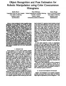
Latent-Class Hough Forests for 3D Object Detection and Pose Estimation Alykhan Tejani, Danhang Tang, Rigas Kouskouridas, and Tae-Kyun Kim Imperial Collge London {alykhan.tejani06, d.tang11, r.kouskouridas, tk.kim}@imperial.ac.uk

Abstract. In this paper we propose a novel framework, Latent-Class Hough Forests, for 3D object detection and pose estimation in heavily cluttered and occluded scenes. Firstly, we adapt the state-of-the-art template matching feature, LINEMOD [14], into a scale-invariant patch descriptor and integrate it into a regression forest using a novel template-based split function. In training, rather than explicitly collecting representative negative samples, our method is trained on positive samples only and we treat the class distributions at the leaf nodes as latent variables. During the inference process we iteratively update these distributions, providing accurate estimation of background clutter and foreground occlusions and thus a better detection rate. Furthermore, as a by-product, the latent class distributions can provide accurate occlusion aware segmentation masks, even in the multi-instance scenario. In addition to an existing public dataset, which contains only single-instance sequences with large amounts of clutter, we have collected a new, more challenging, dataset for multiple-instance detection containing heavy 2D and 3D clutter as well as foreground occlusions. We evaluate the Latent-Class Hough Forest on both of these datasets where we outperform state-of-the art methods.

1

Introduction

Accurate localization and pose estimation of 3D objects is of great importance to many higher level tasks such as robotic manipulation, scene interpretation and augmented reality to name a few. The recent introduction of consumer-level depth sensors have allowed for substantial improvement over traditional 2D approaches as finer 3D geometrical features can be captured. However, there still remain several challenges to address including heavy 2D and 3D clutter, large scale and pose changes due to free-moving cameras as well as partial occlusions of the target object. In the field of 2D object detection, part or patch-based methods, such as Hough Forests [10], have had much success. In addition to being robust against foreground occlusions, they remove detection disambiguation by clustering votes over many local regions into mutually consistent hypothesis. Furthermore, these methods typically separate foreground regions from background clutter/occluders by a discriminatively learnt model, additionally reducing the rate of false positives. However, for practical use, this requires the collection of a representative negative training set which is also able to generalize to unseen environments. At present there is a huge disparity in the number

2

Tejani et al.

of RGB-D image datasets vs. 2D image datasets and furthermore, it is not clear how to select such a representative set in order to not create a unintentional bias to particular environments. In fact, many studies have shown that classifiers can show a significant drop in performance when evaluated on images outside of the training domain [35, 6, 27].

RGB-D images

#iterations=0

#iterations=2

#iterations=10

Fig. 1. An illustration of the algorithm used to update the latent class distributions. Columns 24 show intermediate results from different number of iterations of the algorithm, where row 1 shows the foreground confidence map, Z, and row 2 shows the resulting Hough voting space. Note the contrast of the vote images have been enhanced for visualization.

State-of-the-art approaches in 3D detection and pose estimation [7, 16] avoid this issue by training just from 3D models of the target object. Whilst previously the requirement of 3D models may have been a disadvantage, with recent innovations in surface reconstruction techniques [24, 36] these can now be obtained easily and efficiently using hand-held RGB-D cameras. Using these models, 3D features, either simple pointpair features [7] or holistic templates [16] are extracted from the model and matched to the scene at test time providing promising results, even for texture-less objects in heavily cluttered environments. While these results are encouraging, these methods have only been evaluated under little or no occlusion and under the assumption of only one instance present per image. However, as these methods have no knowledge of the background distribution in training, heavy background clutter can cause false regions to have significant responses. While this is a more prominent issue in the point-to-point methods, as planar regions of target objects are easily matched to background clutter, holistic template matching is by no means immune to this. Motivated by these issues, we present the Latent-Class Hough Forest; a framework for 3D object detection and pose estimation. Unlike the traditional Hough Forest [10], which explicitly exploits classification labels during training, we train only from positive samples and use only the regression term. However, unlike a regression forest [8] we maintain class distributions at leaf nodes. During testing, these distributions are considered as latent variables that are iteratively updated, providing more accurate voting results. Furthermore, as a by-product, our method also produces accurate occlusion-

Latent-Class Hough Forests for 3D Object Detection and Pose Estimation

3

aware figure-ground segmentation masks, which are useful for further post-processing procedures such as efficient occlusion-aware registration [38]. Fig. 1 illustrates this iterative procedure, the effect it has on the output voting results and the figure-ground segmentation masks. Our main contributions can be summarized as follows: – We propose the Latent-Class Hough Forest, a novel patch-based approach to 3D object detection and pose estimation; It performs one-class learning at the training stage, and iteratively infers latent class distributions at test time. – We adapt the state-of-the-art 3D holistic template feature, LINEMOD [14], to be a scale invariant patch descriptor and integrate it into the random forest framework via a novel template-based splitting function. – During the inference stage, we jointly estimate the objects 3D location and pose as well as a pixel wise visibility map, which can be used as an occlusion aware figure-ground segmentation for result refinement. – We provide a new, more challenging public dataset for multi-instance 3D object detection and pose estimation, comprising near and far range 2D and 3D clutter as well as foreground occlusions In the remainder of this paper we first discuss related work in Sec. 2 before introducing our method in Sec. 3. Following this, in Sec. 4, we provide a quantitative and qualitative analysis of our results as well as a comparison to current state-of-the art methods. Finally, in Sec. 5, we conclude with some final remarks and a discussion of future work.

2

Related Work

Throughout the years, several techniques for the detection and registration of objects have been proposed. From the literature, two main categories can be distinguished; nearest-neighbour approaches and learning based methods. Nearest neighbour methods can take a more local approach, such as feature matching, or a holistic approach such as template matching. Local approaches comprise of matching local 2D textural features or 3D geometrical features and transferring their spatial information to form a consistent object hypothesis [7, 18, 4, 20]. On the other hand, template matching approaches [15, 31, 14, 28] attempt to match global descriptors of the object to the scene; These templates can further be used to transfer contextual knowledge, such as 3D pose [16], to the detection. While, feature-point matching is inherently more robust to foreground occlusion, template matching has also been extended to incorporate occlusion reasoning, one notable work being [17]. However, these approaches makes strong assumptions about the occluder shape and location and may not generalize as well. Learning based methods also comprise of local [10, 25, 9] and holistic [5, 32] approaches. Learning based methods tend to quantize samples together and in turn often can generalize better to slight variations in translation, local shape and viewpoint. Furthermore, as an explicit background/foreground separation is learnt parametrically, these methods are geared to work in the presence of heavy background clutter, causing far less false positives than nearest neighbour approaches. However, the efficacy of this

4

Tejani et al.

is heavily dependent on how representative the background training data is of the “real world”, and this benefit does not always transfer across different domains. In fact, it has been shown that significant performance degradation can occur when the negative training set is not representative of target domain [35, 6, 27]. One-class classification is a branch of learning based methods focussed on learning only from positive samples. This branch of learning, first coined by by Moya et al.[23] and further developed by Tax [34] try to learn closed decision boundaries around the target class in the feature space. However, as observed by Tax, these methods suffer from the added issue of specifying the multi-dimensional margin of such a boundary to balance between false positives and negatives and incorrect assignment can significantly affect performance [34]. We refer the reader to [19] for an in-depth review of one-class classification techniques.

3

Proposed Method

Our goal is to achieve accurate 3D object detection and pose estimation via one-class training, whilst being robust to background clutter and foreground occlusions. To this end, we use only synthetic renderings of a 3D model for training. To leverage the inherent robustness to foreground occlusions, we adopt the state-of-the-art patch-based detector, Hough Forests [10], and for the patch representation we use the state-of-theart 3D template descriptor, LINEMOD [14]. However, combining these components naively does not work for the following reasons: i) The absence of negative training data means that we cannot leverage the classification term of the Hough Forest, thus, relinquishing the ability to filter out false results caused by background clutter. ii) It is not clear how to integrate a template-based feature into the random forest framework; The main issue is that the synthetic training images have null space in the background whereas the testing patches will not. Thus, doing a naive holistic patch comparison, or the two-dimenson/ two-pixel tests (as used in [29, 8, 33]) can lead to test patches taking the incorrect route at split functions. iii) LINEMOD [14], in its current form, is not a scale-invariant descriptor; this gives rise to further issues, such as should we train detectors for multiple scales and how finely should we sample these scales in both the training and testing phases. To address these issues, we propose the Latent-Class Hough Forest (LCHF); an adaptation of the conventional Hough Forest that performs one-class learning at the training stage, but uses a novel, iterative approach to infer latent class distributions at test time. In Sec. 3.1 we discuss how to build a LCHF, in particular we discuss how to adapt LINEMOD into a scale-invariant feature and how to integrate it into the random forest framework via a novel template-based split function. Following this, In Sec 3.2, we discuss how testing is performed with the LCHF and how we can iteratively update the latent class distributions and use them to refine our results. 3.1

Learning

Latent-Class Hough Forests are an ensemble of randomized binary decision trees trained using the general random forest framework [2]. During training, each tree is built using

Latent-Class Hough Forests for 3D Object Detection and Pose Estimation

5

a random subset of the complete training data. Each intermediate node in the tree is assigned a split function and threshold to optimize a measure of information gain; this test is then used to route incoming samples either left or right. This process is repeated until some stopping criteria is met, where a leaf node containing application-specific contextual information is formed. Each stage in this learning process is highly application dependent and we will discuss each in turn below.

Training Data In order to capture reasonable viewpoint coverage of the target object, we render synthetic RGB and depth images by placing a virtual camera at each vertex of a subdivided icosahedron of a fixed radius, as described in [13]. A tree is trained from a set of patches, {Pi = (ci , Di , Ti , θi )}, sampled from the training images, where ci = (xi , yi ) is the central pixel, Di is the raw depth map of the patch, Ti is the template describing the patch and θi = (θx , θy , θz , θya , θpi , θro ) is the 3D offset from the patch center to the object center and the 3 Euler angles
representing the object pose. The patch template is defined as Ti = {Oim }m∈M , ∆i , where Oim are the aligned reference patches for each modality, m, which are either the image gradient or normal vector orientations and ∆i = {(r, m)}, where r = (λ · x, λ · y) is a discrete set of pairs made up of the 2D offsets (x, y) scaled by λ which is equal to the templates depth at the central pixel, and modalities, m, of the template features. The template features are evenly spread across the patch; features capturing the image gradients are taken only from the object contours and features capturing the surface normals are taken from the body of the object, the collection and representation of template features is the same as described in [14].

Split Function Given a set of patches, S, arriving at a node, a split function, hi , is created by choosing a random patch, Pi , and evaluating its similarity against all other patches, Pj ∈ S. Along with a randomly chosen threshold, τi , the incoming patches can be split into two distinct subsets Sl = {Pj |hi (Pj ) ≤ τi } and Sr = S \ Sl . The original similarity measure of [14], adapted to work over patches, is formulated as:

ε (Pi , Pj ) =

∆i  X (r,m)

max fm Oim t∈R(cj +r)

(ci +

r) , Ojm


(t)

 (1)

where R(x) defines a small search window centred at location x and fm Oim (x) , Ojm (y) computes the dot product between quantized orientations at locations x and y for modality, m. Note, for clarity we keep the max operator and the explicit function, fm in the formulation, however, we refer the reader to [14] for a discussion on how to compute these with constant time complexity using pre-processing techniques. As neither the patch description, Pi , nor the similarity measure, ε, account for scale, this similarity measure will only work if the patches, Pi and Pj are of the same scale. To remedy this, inspired by [29], we achieve scale-invariance by using the depth of the patch center to scale the offsets, r. More formally, we define a scale-invariant similarity




6

Tejani et al.

measure, ε0 , as:   ε0 (Pi , Pj )



∆i P

=

max

(r,m)

 ς (c , r) x x

= cx +

t∈R(ςj (cj +r))

fm Oim (ςi (ci + r)) , Ojm (t)




 ,

(2)

r Dx (cx )

where Dx (a) is the depth value at location a in patch Px . This similarity measure is still not sufficient, as given two patches, both representing the same part of the target object, one synthetically generated and one from a testing m image (containing background noise), the functions fm (Oim (ςi (ci + r)) , Otrain (t)) m m and fm (Oi (ςi (ci + r)) Otest (t)) will produce significantly different values if any template features, (r, m) ∈ ∆i , from the selected template falls in the null, background, space in the training patch or on to a foreground occluder in the testing patch. This can then cause the two patches to proceed down the tree in different directions, see Fig. 2 for an illustration of this issue. To this end, we alter the similarity function is as follows:   ε00 (Pi , Pj )

=

∆i P (r,m)

 ι (P , P , r) i j

 max

ι(Pi , Pj , r) ·

t∈R(ςj (cj +r))

fm Oim

(ςi (ci +

r)) , Ojm


(t) ,

(3)

= δ (||Di (ςi (ci + r)) − Di (ci )| − |Dj (ςj (cj + r)) − Dj (cj )|| < )

where ι(Pi , Pj , r) is an indicator function that removes template features that are not spatially consistent with the patch’s 3D surface from having an effect on the similarity score. The efficacy of this indicator function is illustrated in Fig 2. Finally, we can express the split function of a node as hi (Pj ) = ε00 (Pi , Pj ). The effectiveness of a particular splitting function is evaluated by the information gain, however, as no negative data is present at training we cannot use the formulation of the Hough Forest [10]. Instead, we measure only the entropy of the offset and pose regression as done in the regression forest of Fanelli et al.[8]. This process is then repeated multiple times and the split, (hi , τi ), producing the highest information gain is selected as the nodes split function. Constructing Leaf Nodes The training data is recursively split by this process until the tree has reached a maximum depth or the number of samples arriving at a node fall below a threshold. When this criteria is met a leaf node is formed from the patches reaching it. The leaf node stores votes for both the center position of the object, (θx , θy , θz ), and the pose, (θya , θpi , θro ). Following the approach of Girshick et al.[11] we only store the modes of the distribution which we find efficiently via the mean shift algorithm. Finally, similar to the Hough Forest [10], we create a class distribution at the leaf, however, as no background information reaches the leaves during training this distribution is initialized to pf g = 1 and pbg = 0 for the foreground and background probabilities respectively. 3.2

Inference

We want to estimate the probability of the random event, E(θ), that the target object exists in the scene under the 6 degrees of freedom pose θ = (θx , θy , θz , θya , θpi , θro ).

Latent-Class Hough Forests for 3D Object Detection and Pose Estimation

7

Fig. 2. A conceptual view of how our similarity measurement works. Left: rows 1 & 2 show two patches, one from training and one from testing; both are of different scale which is handled by Eq 2. Row 3 shows the learnt template, T , at the highlighted node. Right: Shows how without the indicator function (Eq 3) the two patches can go down different paths in the tree, leading to wrong results.

We can calculate this by aggregating the conditional probabilities P (E(θ)|P) for each patch, P. As we only model the effect that positive patches have on the pose estimation, the existence of an estimation at θ in the pose space assumes the vote originates from a foreground patch, that is pf g = 1, which is assumed for all patches initially. Thus, for a patch P evaluated on tree T and reaching leaf node l, we can formalise the conditional probability as:
p (E (θ) |P; T ) = p E (θ) , plf g = 1|P (4)

= p E (θ) |plf g = 1, P · p plf g = 1|P where plf g is the foreground probability at the leaf node, l. Finally, for a forest, F, we simply average the probabilities over all trees: |F |

p (E (θ) |P; F) =

1 X p (E (θ) |P; Tt ) |F| t

(5)

The first factor, p (E (θ) |pf g = 1, P), can be estimated by passing each patch down the forest and accumulating the votes stored at the leaf, in which votes from multiple trees can be combined in an additive manner, this gives us the same probabilities as in Eq. 5 up to a constant factor. The estimation is then deferred to the ability of locating local maxima in this aggregated space which, traditionally, has been done by either exhaustively searching the space combined with non-max suppression or by treating each vote as a point in the space and using mean shift to locate the modes. However,

8

Tejani et al.

these approaches are usually applied to low dimensional (2D) spaces [10, 26, 21] or in cases where many of the data points (pixels) have already been removed via some preprocessing [8, 33]. In our case, the pose voting space is 6 dimensional and in the case of evaluating all patches in a VGA image for several trees in the forest, the number of data points becomes very large and this solution is highly inefficient. To this end, we propose a three-stage localization technique; We initially aggregate all votes into a 2D voting space i.e. p (E ((θx , θy )) |P) and use this space to locate the hypothesis with non-max suppression. We then further process the votes from patches within the bounding box of these hypothesis to locate modes in the 3D translation space, (θx , θy , θz ), and finally use the patches to find the modes in the rotation space, (θya , θpi , θro ), given the estimated translation. The second factor of Eq (4), p (pf g = 1|P), is traditionally estimated from the learnt class distribution at the leaf nodes. However, in the LCHF this is a latent distribution and all leaf nodes are in initially set to have pf g = 1. Therefore, we propose a method similar to the co-training concept to iteratively update these distributions from the observable unlabelled data in the scene. Co-training [1] is a technique, that has seen much success in many applications [22, 3, 37], where the main idea is to have two independent classifiers, in which each iteratively predicts labels for the unlabelled data and then uses these labels to update the other classifier. In the seminal work of Blum & Mitchell [1] it was stated that each classifier should be trained from different views/feature representations of the data, but it was later shown that using two classifiers trained originally on the same view will suffice [12], and this is the variant most similar to our method. Thus, to obtain classifiers, for each iteration of the co-training, we randomly partition the random forest, F, into two forest subsets, F1 & F2 , which can be seen as independent classifiers in their own right. Following this, given a forest, F, we select a random subset of the image patches and predict  their labels by evaluating Eq (4) to obtain an initial object hypotheses set, Θ = θi . For the N most likely hypotheses, we backproject the contributing votes to their corresponding patches to obtain a consensus patch set, Ki as done in [20]. This patch set is then further reduced to a consensus pixel set, Π, as follows: !

  Π  

g Pj , θ

=
i

S

S

θ i ∈Θ

Pj ∈Ki

g Pj , θ

i




,

(6)

= {pj ∈ Pj |d (cj , θi ) ≤ α ∧ d(pj , cj ) ≤ β}

where pj are pixels, d is the euclidean distance function,  is the diameter of the target objects 3D model and α and β are scaling coefficients. The consensus pixel set contains the pixels from patches that vote for the selected hypotheses and are also spatially consistent with the hypothesis that they vote for. All pixels in Π are then labelled as foreground pixels and all others as background, thus producing two labelled datasets from the patches extracted around those pixels, P + and P − . These datasets are then passed as input to the second classifier, Fj , where each leaf node, l, accumulates the patches that arrive at it, Pl , and updates the leaf

Latent-Class Hough Forests for 3D Object Detection and Pose Estimation

9

probability distribution as follows: plf g =

| {Pi | Pi ∈ (Pl ∩ P + )} | |Pl |

(7)

This process is then repeated for a fixed number of iterations. Once finished, the final hypotheses set is produced by passing all patches down the complete forest, F and evaluating Eq (5) using the newly learnt plf g . The overall principle of this co-training algorithm is depicted in Algorithm 1 and in Fig. 1.

Algorithm 1 Update Latent-Class Distributions Require: An input image, I; A Latent-Class Hough Forest, F 1: repeat 2: Randomly draw a subset of trees Fi from F; Fj = F \ Fi . 3: Randomly sample a set of patches P from I. 4: Propagate P down Fi collect hypotheses set Θ with Eq (5). 5: Backproject top N hypotheses to obtain a consensus set Π (Eq. (6)). 6: Partition P ∈ P into positive and negative sets using the consensus set. P + = {P|P ∈ Π} P− = P \ P+ 7: Propagate P + and P − down Fj and update the leaf node distributions with Eq (7). 8: until Maximum iteration

Additionally, as a by-product of this process, we can produce a pixel-wise foreground confidence map, Z, of the input image by labelling each pixel by the average plf g (see Fig 1). Using the confidence map, Z, and the final set of hypotheses, Θ, we can produce a final image segmentation mask, M, by M=

[



B θi ∩ Z

(8)

θ i ∈Θ

where B (θ) is a function that computes the bounding box from the hypothesis θ. This final segmentation, although not currently used, is useful for further refinement of the hypotheses, for example by using it as input for an occlusion-aware ICP alignment.

4

Experiments

We perform experiments on two 3D pose estimation datasets. The first is the publicly available dataset of of Hinterstoisser et al.[16], which contains 13 distinct objects each associated with an individual test sequence comprising of over 1,100 images with close and far range 2D and 3D clutter. Each test image is annotated with ground truth position and 3D pose.

10

Tejani et al.

For further experimentation, we propose a new dataset consisting of 6 additional 3D objects. We provide a dense 3D reconstruction of each object obtained via a commercially available 3D scanning tool [30]. For each object, similarly to [16], we provide an individual testing sequence containing over 700 images annotated with ground truth position and 3D pose. Testing sequences were obtained by a freely moving handheld RGB-D camera and ground truth was calculated using marker boards and verified manually. The testing images were sampled to produce sequences that are uniformly distributed in the pose space by [0◦ − 360◦ ], [−80◦ − 80◦ ] and [−70◦ − 70◦ ] in the yaw, roll and pitch angles respectively. Unlike the dataset of [16], our testing sequences contain multiple object instances and foreground occlusions in addition to near and far range 2D and 3D clutter, making it more challenging for the task of 3D object detection and pose estimation. Some example frames from this dataset can be seen in Fig 5. In Sec. 4.1 we perform self comparison tests highlighting the benefits of adding scale-invariance to the template similarity measure (Eq. (2)) and using co-training to update the latent class distributions (Algorithm 1). Following this, in Sec. 4.2 we present a comparison of our method against the state of the art methods, namely LINEMOD [14] and the method of Drost et al.[7]. In all tests we use the metric defined in [16] to determine if an estimation is correct. More formally, for a 3D model M, with ground truth rotation R and translation T , ˆ and translation, Tˆ, the matching score is defined as given an estimated rotation, R ˆ + Tˆ)|| m = avg ||(Rx + T ) − (Rx

(9)

x∈M

for non-symmetric objects and ˆ 2 + Tˆ)|| m = avg min ||(Rx1 + T ) − (Rx x1 ∈Mx2 ∈M

(10)

for symmetric objects. An estimation is deemed correct if m ≤ km d, where km is a chosen coefficient and d is the diameter of M. Unlike [14], in which only the top N detections from each image are selected, we compute precision-recall curves and present the F1-Score which is the harmonic mean of precision and recall. We argue that this is a more accurate form of comparison, as directly comparing detections is inaccurate as some images may be harder than others, which is especially true in the case of occlussion and heavy clutter (as in our new dataset). Therefore, similarly to [28], we argue a more meaningful evaluation is to sort all detection scores across all images and calculate the general performance of the detector, given by the precision-recall curves. In all experiments, unless otherwise stated, the parameters for our method are as follows. For each object class we train a Latent-Class Hough Forest comprising of 10 trees with a maximum depth of 25 trained from randomly selected set of training patches. Image patch templates centred at a pixel consist of 20 features in both the color gradient and normal channel. These features are selected anywhere in a search window centred at the central pixel with a maximum size of, but not further than, 31 of the bounding box size in any direction and are chosen randomly in the same method as described in [14]. For the co-training stage we set the number of iterations empirically as 10 and the number of hypothesis to be backprojected per iteration as N = 5. We choose 5 as it

Latent-Class Hough Forests for 3D Object Detection and Pose Estimation

11

is greater than the number of instances present in all datasets, however this number is not fixed and can be adapted based on application. Furthermore, in all experiments the coefficient km is set to the value of 0.15, the results with this coefficient are also found to be visually correct. 4.1

Self Comparisons

We perform two self comparisons on the dataset of Hinterstoisser et al.[16]. Firstly we compare the results of our method with and without updating the latent class distributions. As can be seen in Fig. 3 our approach with updating distributions improves the F1-Score by 2.8% on average and up to 8.2% on some objects. The biggest gains are seen in objects which have large amounts of indistinct planar regions, for which background clutter can easily be confused at the patch level. For example, the biggest improvements are seen in the Camera, Holepuncher and Phone objects which contain large planar regions. Furthermore, in Fig. 3 we also compare the results of LINEMOD [14] using holistic templates with the original similarity measure (Eq. (1)) and the scaleinvariant similarity measure (Eq. (2)). As the scale-invariant version is trained using only one scale, the performance is increased 6-fold (623 templates as opposed to 3738). Furthermore, the performance is also increased by 7.2% on average, this is due to the fact that templates are able to be matched at scales not seen in the template learning stage of the original LINEMOD [14]. Comparison on the dataset of Hinterstoisser et al.[16]

Fig. 3. F1-Scores for the 13 objects in the dataset of Hinterstoisser et al.[16]. We compare our approach with and without updating the latent class variables (Sec. 3.2). We additionally show results of the scale-invariant LINEMOD templates vs. the original LINEMOD templates [14].

4.2

Comparison to State-of-the-arts

We compare our method to two state-of-the-art methods, namely LINEMOD [14] and the method of Drost et al.[7]. For LINEMOD, we use our own implementation based on [14] and for the method of Drost et al.[7], we use a binary version kindly provided by the author and set the parameters to the recommended defaults. Furthermore, for the

12

Tejani et al.

method of Drost et al.[7] we remove points further than 2000mm to reduce the effect of noise, as recommended by the authors. Note, this should not effect accuracy as all target objects are safely within this range. In Fig. 4 we show the average precision-recall curves across all objects in both datasets respectively and in Tables 1 and 2 we show the F1-Score per object for each dataset. All methods show worse performance on the new dataset, which is to be suspected due to the introduction of occlusions as well as multiple object instances. As can be seen we outperform both state-of-the-arts in both datasets. However, a point to note is that by just picking the top detection from each image, as done in [16], the method of Drost et al.[7] and LINEMOD [14] are shown to be almost equal in accuracy (see [16] for this comparison), however, when considering the precision-recall curve, as we do, the method of Drost et al.has considerably lower precision values. This is due to the fact that this method does not take object boundaries into consideration, thus large planar regions of the target object can have a large surface overlap in the background clutter causing many false positives in addition to the true positives. Conversely, our method maintains high levels of precision at high recall which is due to the inferred latent class distributions simplifying the Hough space. In Fig. 5 we present some qualitative results on both datasets.

(a)

(b)

Fig. 4. Average Precision-Recall curve over all objects in the dataset of LINEMOD [16] (a) and our dataset (b). The shaded region represents one standard deviation above and below the precision value at a given recall value.

5

Conclusion

In this paper we have introduced a novel framework for accurate 3D detection and pose estimation of multiple object instances in cluttered and occluded scenes. We have demonstrated that these challenges can be efficiently met via the adoption of a state-ofthe-art template matching feature into a patch-based regression forest. During training

Latent-Class Hough Forests for 3D Object Detection and Pose Estimation Approach Sequence (# images) Ape(1235) Bench Vise (1214) Driller (1187) Cam (1200) Can (1195) Iron (1151) Lamp (1226) Phone (1224) Cat (1178) Hole Punch (1236) Duck (1253) Box (1252) Glue (1219) Average (15770)

LINEMOD [14] 0.533 0.846 0.691 0.640 0.512 0.683 0.675 0.563 0.656 0.516 0.580 0.860 0.438 0.630

Drost et al.[7] F1-Score 0.628 0.237 0.597 0.513 0.510 0.405 0.776 0.471 0.566 0.500 0.313 0.826 0.382 0.517

13

Our Approach 0.855 0.961 0.905 0.718 0.709 0.735 0.921 0.728 0.888 0.875 0.907 0.740 0.678 0.817

Table 1. F1-Scores for LINEMOD [14], the method of Drost et al.[7] and our approach for each object class for the dataset of Hinterstoisser et al.[16].

Approach Sequence (# images) Coffee Cup (708) Shampoo (1058) Joystick (1032) Camera (708) Juice Carton (859) Milk (860) Average (5229)

LINEMOD [14] 0.819 0.625 0.454 0.422 0.494 0.176 0.498

Drost et al.[7] F1-Score 0.867 0.651 0.277 0.407 0.604 0.259 0.511

Our Approach 0.877 0.759 0.534 0.372 0.870 0.385 0.633

Table 2. F1-Scores for LINEMOD [14], the method of Drost et al.[7] and our approach for each object class for our new dataset [16].

we employ a one-class learning scheme, i.e. training with positive samples only rather than involving negative examples. In turn, during inference, we engage the proposed Latent-Class Hough Forest that iteratively produces a more accurate estimation of the clutter/occluder distribution by considering class distribution as latent variables. As a result, apart from accurate detection results we can, further, obtain an highly representative occlusion-aware masks facilitating further tasks such as scene layout understanding, occlusion aware ICP or online domain adaption to name a few. Our method is evaluated using both the public dataset of Hinterstoisser et al. [16] and our new challenging one containing foreground occlusion and multiple object instances. Experimental evaluation provides evidence of our novel L-C Hough Forest outperforming all baselines highlighting the potential benefits of part-based strategies to address the issues of such a challenging problem.

14

Tejani et al.

Fig. 5. Some qualitative results on both datasets. Rows 1-6 show, from left to right, the original RGB image, the final segmentation mask, the final Hough vote map and the augmented 3D axis of the estimated result. The final row shows some incorrect results.

Acknowledgement This project was supported by the Omron Corporation.

Latent-Class Hough Forests for 3D Object Detection and Pose Estimation

15

References 1. Blum, A., Mitchell, T.: Combining labeled and unlabeled data with co-training. In: COLT. ACM (1998) 2. Breiman, L.: Random forests. Machine learning (2001) 3. Chan, J., Koprinska, I., Poon, J.: Co-training with a single natural feature set applied to email classification. In: WIC (2004) 4. Choi, C., Christensen, H.I.: 3d pose estimation of daily objects using an rgb-d camera. In: IROS (2012) 5. Dalal, N., Triggs, B.: Histograms of oriented gradients for human detection. In: CVPR (2005) 6. Doll´ar, P., Wojek, C., Schiele, B., Perona, P.: Pedestrian detection: A benchmark. In: CVPR (2009) 7. Drost, B., Ulrich, M., Navab, N., Ilic, S.: Model globally, match locally: Efficient and robust 3d object recognition. In: CVPR (2010) 8. Fanelli, G., Gall, J., Van Gool, L.: Real time head pose estimation with random regression forests. In: CVPR (2011) 9. Felzenszwalb, P.F., Girshick, R.B., McAllester, D., Ramanan, D.: Object detection with discriminatively trained part based models. PAMI (2010) 10. Gall, J., Yao, A., Razavi, N., Van Gool, L., Lempitsky, V.: Hough forests for object detection, tracking, and action recognition. PAMI (2011) 11. Girshick, R., Shotton, J., Kohli, P., Criminisi, A., Fitzgibbon, A.: Efficient regression of general-activity human poses from depth images. In: Computer Vision (ICCV), 2011 IEEE International Conference on. pp. 415–422. IEEE (2011) 12. Goldman, S., Zhou, Y.: Enhancing supervised learning with unlabeled data. In: ICML (2000) 13. Hinterstoisser, S., Benhimane, S., , Lepetit, V., Navab, N.: Simultaneous recognition and homography extraction of local patches with a simple linear classifier (2008) 14. Hinterstoisser, S., Holzer, S., Cagniart, C., Ilic, S., Konolige, K., Navab, N., Lepetit, V.: Multimodal templates for real-time detection of texture-less objects in heavily cluttered scenes. In: ICCV (2011) 15. Hinterstoisser, S., Lepetit, V., Ilic, S., Fua, P., Navab, N.: Dominant orientation templates for real-time detection of texture-less objects. In: CVPR (2010) 16. Hinterstoisser, S., Lepetit, V., Ilic, S., Holzer, S., Bradski, G., Konolige, K., Navab, N.: Model based training, detection and pose estimation of texture-less 3d objects in heavily cluttered scenes. In: ACCV (2012) 17. Hsiao, E., Hebert, M.: Occlusion reasoning for object detection under arbitrary viewpoint. In: CVPR (2012) 18. Johnson, A.E., Hebert, M.: Using spin images for efficient object recognition in cluttered 3d scenes. PAMI (1999) 19. Khan, S.S., Madden, M.G.: One-class classification: Taxonomy of study and review of techniques. arXiv preprint arXiv:1312.0049 (2013) 20. Leibe, B., Leonardis, A., Schiele, B.: Combined object categorization and segmentation with an implicit shape model. In: ECCV (2004) 21. Leibe, B., Leonardis, A., Schiele, B.: Robust object detection with interleaved categorization and segmentation. IJCV (2008) 22. Liu, R., Cheng, J., Lu, H.: A robust boosting tracker with minimum error bound in a cotraining framework. In: ICCV (2009) 23. Moya, M., Koch, M., Hostetler, L.: One-class classifier networks for target recognition applications. Tech. rep. (1993)

16

Tejani et al.

24. Newcombe, R.A., Davison, A.J., Izadi, S., Kohli, P., Hilliges, O., Shotton, J., Molyneaux, D., Hodges, S., Kim, D., Fitzgibbon, A.: Kinectfusion: Real-time dense surface mapping and tracking. In: Mixed and augmented reality (ISMAR), 2011 10th IEEE international symposium on. pp. 127–136. IEEE (2011) 25. Okada, R.: Discriminative generalized hough transform for object dectection. In: ICCV (2009) 26. Opelt, A., Pinz, A., Zisserman, A.: Learning an alphabet of shape and appearance for multiclass object detection. IJCV (2008) 27. Perronnin, F., S´anchez, J., Liu, Y.: Large-scale image categorization with explicit data embedding. In: CVPR (2010) 28. Rios-Cabrera, R., Tuytelaars, T.: Discriminatively trained templates for 3d object detection: A real time scalable approach. In: ICCV (2013) 29. Shotton, J., Sharp, T., Kipman, A., Fitzgibbon, A., Finocchio, M., Blake, A., Cook, M., Moore, R.: Real-time human pose recognition in parts from single depth images. ACM (2013) 30. Skanect: skanect.manctl.com/ (2014) 31. Steger, C.: Similarity measures for occlusion, clutter, and illumination invariant object recognition. In: Pattern Recognition, pp. 148–154. Springer (2001) 32. Tang, D., Liu, Y., Kim, T.K.: Fast pedestrian detection by cascaded random forest with dominant orientation templates. In: BMVC (2012) 33. Tang, D., Yu, T.H., Kim, T.K.: Real-time articulated hand pose estimation using semisupervised transductive regression forests. In: ICCV (2013) 34. Tax, D.M.: One-class classification (2001) 35. Torralba, A., Efros, A.A.: Unbiased look at dataset bias. In: CVPR (2011) 36. Weise, T., Wismer, T., Leibe, B., Van Gool, L.: In-hand scanning with online loop closure. In: Computer Vision Workshops (ICCV Workshops), 2009 IEEE 12th International Conference on. pp. 1630–1637. IEEE (2009) 37. Yu, S., Krishnapuram, B., Rosales, R., Steck, H., Rao, R.B.: Bayesian co-training. In: NIPS (2007) 38. Zhang, Z.: Iterative point matching for registration of free-form curves and surfaces. International journal of computer vision 13(2), 119–152 (1994)