We describe an approach to category-level detection and viewpoint estimation for rigid 3D objects from single 2D images. In contrast to many existing methods, ...
Viewpoint-Aware Object Detection and Pose Estimation Daniel Glasner1 , Meirav Galun1 , Sharon Alpert1 , Ronen Basri1 , and Gregory Shakhnarovich2 1
Department of Computer Science and Applied Mathematics, The Weizmann Institute of Science 2 Toyota Technological Institute at Chicago
Abstract We describe an approach to category-level detection and viewpoint estimation for rigid 3D objects from single 2D images. In contrast to many existing methods, we directly integrate 3D reasoning with an appearance-based voting architecture. Our method relies on a nonparametric representation of a joint distribution of shape and appearance of the object class. Our voting method employs a novel parametrization of joint detection and viewpoint hypothesis space, allowing efficient accumulation of evidence. We combine this with a re-scoring and refinement mechanism, using an ensemble of view-specific Support Vector Machines. We evaluate the performance of our approach in detection and pose estimation of cars on a number of benchmark datasets.
1. Introduction The problem of category-level object detection has been at the forefront of computer vision research in recent years. One of the main difficulties in the detection task stems from variability in the objects’ appearance due to viewpoint variation (or equivalently pose variation). While most existing methods treat the detection task as that of 2D pattern recognition, there is an increasing interest in methods that explicitly account for view variation and that combine detection with pose estimation. This paper presents an approach that integrates detection and pose estimation using 3D class models of rigid objects and demonstrates this approach on the problem of car detection. Building a viewpoint-aware detector presents a number of challenges. The first question is how to acquire a 3D representation of a class. The recent availability of CAD modResearch was supported in part by the Vulcan Consortium funded by the Magnet Program of the Israeli Ministry of Commerce, Trade and Labor, Chief Scientist Office. The vision group at the Weizmann Institute is supported in part by the Moross Laboratory for Vision Research and Robotics.
els, 3D cameras, and robust structure-from-motion (SfM) software have simplified this problem. Using SfM methods or 3D cameras makes it straightforward to relate the available 3D representations to the appearance of objects in training images. Secondly, finding the pose of an object at test time requires search in the 6D space of possible Euclidean transformations. This can be accomplished by searching exhaustively through a discrete binning of this 6D space. An alternative is to use a combinatorial search (e.g. RANSAC [7]) procedure. Both options, however, can be computationally expensive. Finally, how should detection and pose estimation be integrated? Pose estimation can deteriorate significantly when detection is inaccurate. Can detection be improved if pose estimation is integrated into the process? We suggest an approach that combines a nonparametric voting procedure with discriminative re-scoring for detection and pose estimation of rigid objects. We construct a class model by merging 3D shapes of objects, obtained by applying state-of-the-art SFM reconstruction software [19, 8] to a training set that we have collected. A nonparametric voting procedure serves as an attention mechanism to propose candidates for detection. Each image feature can vote for a detection of a class instance along with its 3D pose. These proposed detections are then fed to SVM classifiers to assign a score, refine their location and bounding box, and improve their pose estimates. We focus our experiments on cars and apply our algorithm to four datasets: Pascal 2007, 3D-pose data set [18], EPFL car data set [17], and the data set we have collected and annotated for this work. We present several contributions: • Our efficient voting procedure uses single feature votes to index the 6D space of transformations. • The 6D space of transformation is treated as a continuous space. This allows us to estimate novel poses through a mean-shift mode seeking process. • The combination of our 3D model and the collected
training data allows us to achieve favorable detection and pose estimation results on a variety of publicly available datasets compared to existing, view-aware detection methods.
2. Background A common approach for coping with viewpoint variability is to use multiple, independent 2D models. This multiview approach describes the appearance of an object class at a discrete set of representative viewpoints. These algorithms (e.g., [25, 6, 17, 13]) assume that the 2D appearance of an object near the representative views varies smoothly and that local descriptors are robust enough to handle these appearance variations. [10] extend this approach to allow for continuous viewpoint estimation by learning a linear model around each of the discrete representative views. Another line of studies [18, 24, 21] approaches the problem of view variation by building 2D multi-part representations and establishing correspondences among the parts across different class views. The resulting model accounts for a dense, multiview representation and is capable of recognizing unseen views. Algorithms that utilize 3D CAD models, have been suggested in [15, 20]. To predict the appearance of objects in 2D images from the CAD models, these methods render the CAD models and extract features (e.g., edges) from the rendering. A related work [14], utilizes both CAD and real images, but proposes to treat appearance and geometry as separate learning tasks. In all of these works [15, 14, 20] the pose estimation is limited to a discrete set of viewpoints. In other work, Arie-Nachimson and Basri [1] construct a 3D model by employing an SfM process on the entire training set of class images. Their method requires finding correspondences between parts as they appear in different class instances. Sun et al. [22] suggest the use of depth information, and train models using depth maps acquired with a range camera. Detections are generated by depthencoded voting. Pose estimation is then achieved by registering the inferred point cloud and a 3D CAD model. The Poselets method [3] requires viewpoint invariant annotation of parts in training data, and creates a model by clustering parts based on appearance. Finally, a hybrid 2D-3D model is suggested in [11]. The model consists of stick-like 2D and 3D primitives. The learning selects 3D primitives to describe viewpoint varying parts and 2D primitives where appearance is viewpoint invariant.
3. Nonparametric detection We approach the problem of object detection and pose estimation in two stages. First we apply nonparametric voting to produce a bank of candidate detections along with their estimated poses. Then we apply a discriminative re-
scoring procedure designed to improve the detection and pose estimation results. In this section we describe the construction of a 3D model and the voting in the 6D space of possible pose variables. The re-scoring step is described in Section 4. Hough-like voting procedures have proved effective in object detection both in 2D [12] and in 3D methods [1, 23]. Their success is due to the frequent resemblance of corresponding visual elements across instances of a class. Thus, for example, an image region similar to a stored patch depicting the appearance of a bottom left windshield corner in a previously seen car may indicate the presence of a windshield corner of a (possibly different) car in the test image. Moreover, since appearance can change significantly with viewpoint, such a match may also indicate the viewpoint from which the car is observed. Naturally, such evidence would not be very reliable, as we confine ourselves to small regions. Voting allows us to overcome this by accumulating information from a large number of regions and identifying constellations of patches that cooperatively look like parts of previously seen class instances. These patches are seen from similar viewpoints, and arranged in positions consistent with each other under that viewpoint.
3.1. Model representation The object category of interest is represented by a set of 3D models of object instances. Each single model consists of a cloud of 3D points in a class-centered coordinate frame, i.e., the 3D models of the different class instances are aligned to produce consistent poses. Along with these 3D models we store a collection of regions obtained from the set of training images at different scales. Each image region (patch) is associated with a particular 3D position and a particular viewpoint and scale. These patches are the basic elements of our nonparametric model. Each patch is described by a 3D feature represented as a tuple f 3 = he, l, t, xi, where e is a descriptor of the patch appearance, l is the 3D location of the associated keypoint, and t and x are related to the training image from which the patch associated with f 3 was extracted. t indexes the image and scale, and x is the location of the patch in that image. Note that multiple features will share the same 3D location l, but will have different t values (indicating that they come from different images at different scales) and possibly different appearance e (see Figure 1). We will refer to the entire collection of 3D 3 pooled from all the models as the 3D features f13 , . . . , fD database. Preservation of multiple instances in the model allows us to mix and match parts from different instances, without potential loss of discriminative information associated with quantization, which has been pointed out in [2]. Finally, we include in our model a set of m designated des 3D points P = {pdes 1 , . . . , pm }. For our car model we use m = 4 and select the origin along with three vertices of
Figure 1. 2D appearances An example of the different 2D appearances {e} of a 3D point l (denoted as a green dot) as seen from different view-points and scales (corresponding to different training image indices t)
a cube of side length one half, centered at the origin. We discuss the role of these designated points at greater length below.
3.2. Pose-sensitive voting The objective of the voting step is to identify clusters of features that vote for the class in positions consistent with a particular pose setting. This voting step lies at the core of our method and differs from previously proposed voting schemes in two ways. First, the votes are cast independently by individual features. This is different and more efficient than existing methods that either discretely sample the 6D pose space (and often just a small subset of the subspace) or resort to exhaustive enumeration of subsets of feature constellations in the input. Second, we cope with the non-uniformity of the space of Euclidean transformations (SO(3) × R3 ) by representing the transformations using their effect on the set of designated points, which produces an embedding amenable to a Euclidean norm. As is typical of nonparametric models, most of the computation occurs at test time, when an input image is fed to the detector. The image is covered by an overlapping grid of patches; each patch corresponds to a 2D feature represented by f 2 = he, xi where e is the descriptor extracted from the patch, and x is the 2D coordinates of the patch. An input feature fi2 = hei , xi i “solicits” votes from the instance models, as follows. We find the K nearest neighbors of ei among the descriptors of model patches, and consider the corresponding 3D features to be the matches for 3 fi2 . Without loss of generality, let these be f13 , . . . , fK . A 2 3 match fi = hei , xi i → fk = hek , lk , tk , xk i implies a hypothesized transformation Ti,k , as explained below. In this work we consider the weak perspective projection model: an object undergoes isotropic scaling, 3D rotation
and 2D translation parallel to the image plane, followed by orthographic projection onto the image plane. The scaling is equivalent to translation along the axis orthogonal to image plane prior to projection. Projective transformations in this family have six degrees of freedom (DOF): two for in-plane translation, one for scaling, and three for rotation. We assume that an object point’s appearance is invariant under translation but varies under rotation and scale. We can thus hypothesize that since the patch of fi2 is similar to that of fk3 , the corresponding object point is viewed from the same viewpoint and at the same scale (equivalently translation along the optical axis z). Thus, four out of six DOF of Ti,k can be inferred directly from fk3 (by looking up the scale and viewpoint of the training image indexed by tk ). The remaining two parameters of translation parallel to the image plane are recovered from the equation Ti,k (lk ) = xi . We now need to turn the estimated Ti,k into a vote in the space of transformations. In the spirit of Hough transform, we choose a parametrization for this 6D space, keeping in mind the eventual need to identify peaks and evaluate similarity between votes. We solve this with the help of the designated points, defined in Section 3.1. Specifically, we represent Ti,k as a point in R2m : T des T T V (i, k) = [ Ti,k (pdes 1 ) , . . . , Ti,k (pm ) ] ,
(1)
where {pdes j } denote the designated points in the model and � tk Ti,k (pdes j ) = xi + xj − xk .
(2)
Here xtjk is the projection of the j’th designated point onto the training image indexed by tk . This is illustrated in Fig. 2. Note that the weak perspective assumption allows us to store the locations of the projections of designated points in each training image and simply apply the translation part of Ti,k at test time to generate a vote. We denote by V the set of all the votes cast by features of the input image; if the number of 2D features extracted from the input image is N0 then |V| = K · N0 .
3.3. Vote consolidation Once all votes have been cast, we seek peaks as modes of the estimated density of votes, subject to pose consistency. These can be found by the mean-shift algorithm which climbs the estimated density surface from each vote. We found this to be somewhat slow in practice, and therefore resorted to a multi-stage approximation, described in some detail in Section 5. Finally, we form vote clusters by a greedy procedure. The top ranked mode V10 is associated with the first cluster. In general, V10 is a point in the 2m-dimensional voting space
Figure 2. Voting process. Four patches from the test image (top left) are matched to database patches. The matching patches are shown with the corresponding color on the right column. Each match generates a vote in 6D pose space. We parameterize a point in pose space as a projection of designated points in 3D onto the image plane. These projections are shown here as dotted triangles. The red, green and blue votes correspond to a true detection, the cast pose votes are well clustered in pose space (bottom left) while the yellow match casts a false vote.
which may not correspond to a valid transformation (i.e. it is not obtainable as a projection of the designated points in the weak perspective model). We therefore compute a valid transformation for each mode which maps the designated points to a similar constellation. This is equivalent to the problem of camera calibration from correspondences between m image points in V 0 and their known 3D counterparts in the form of designated points. We solve it as such, using the method in [27] as implemented in the “camera calibration toolbox”, and use the resulting transformation to reproject the designated points onto the test image. We denote this “corrected” mode, now guaranteed to be valid, as V˜ 0 . Now we associate with the cluster represented by V˜ 0 all votes that are sufficiently similar to V˜ 0 in the location of the detected object and the estimated viewpoint (see Section 5 for details). The points associated with the top-ranked mode are culled from the vote set V. The second ranking mode (if it has not been associated with the first cluster) is corrected, and the votes still in V are associated with it based on similarity. The process continues until we have the desired number of clusters or V is empty.
4. Verification, refinement, and rescoring The voting procedure described in the previous section results in a set of hypothesized detections, represented by
V˜10 , . . . , V˜N0 . These are passed to the second stage of our detector, which ranks detection candidates, improves localization and bounding boxes, and resolves opposite viewpoint ambiguities. The overall objective is to improve the precision-recall performance. We cast this as a scoring problem: given a region b in the image, we assign a score value S(b) which is higher the more likely we deem b to be the bounding box of an object instance. This score can be used to classify the region, by thresholding S, and to rank detections, ordering by decreasing value of S. SVM scoring We use Support Vector Machine (SVM) to estimate the score S(b). A region b is represented as a feature vector h(b) which is a concatenation of histograms of oriented gradients computed over a pyramid of spatial bins. We train the SVM on a set of feature vectors {bn } computed from labeled example regions. Details are given in Section 5. Once trained, the SVM score is computed as X S(b) = αn K(h(b), h(bn )) (3) n∈SV
where αn are positive coefficients, SV is a subset of indices of training examples and K is an RBF kernel function � � 1 K(x, x0 ) = exp − 2 k(x − x0 )k22 . σ Viewpoint specific training We can either train a single SVM, or a set of SVMs, designating a separate machine per sector in the viewpoint sphere. Our motivation for choosing the latter is related to the observation, shared by [5], that pose changes may be better fit by a mixture of appearancebased models. In this case, we provide a different set of positive examples to each SVM - namely those in which the correct viewpoint falls within the associated viewpoint region. The set of negative examples is shared across SVMs. At test time we use the viewpoint estimated by the voting procedure to determine which SVM to apply. Given a candidate detection with an estimated viewpoint, we compute the score of the SVM “responsible” for that viewpoint, and its opposite, corresponding to the 180 degree reversal of viewpoint. This is due to the empirical observation that the errors “flipping” the object seem to be far more frequent than other errors in viewpoint estimation. The higher SVM score is used as the detection score and the pose is flipped if this score was produced by the SVM responsible to the flipped direction. Refinement Inspired by [6] we also use the SVM scoring to refine the detection bounding box via local search. Given the initial bounding box b generated by the voting, we consider a set of perturbed versions of b, obtained by a fixed set of shifts and scale changes relative to b. Each of these is scored, and the version with the highest score is used.
5. Experiments We evaluate our approach on the problem of car detection. Below we describe the training data and the model obtained, and report the results on a number of benchmark data sets.
5.1. Training data and the model Data collection and initial model building We collected and processed 22 sets of images of different car models. A set consists of approximately 70 images on average, of one car taken from different viewpoints which cover a full rotation around the car. The pictures were taken in an unconstrained outdoor setting using a hand-held camera. There are significant illumination changes, many images include cars in the background, and in some images the car is cropped or occluded. See Figure 3 (a). Model construction and alignment We use Bundler [19] and PMVS2 software [8] to turn a collection of images of an instance from the class into a model. This yields a set of models with coordinate frames that are somewhat arbitrary. We transform the coordinates so that the object centroid is at the origin, and the coordinate frame is aligned with the three principal components of the 3D point cloud (enforcing a left-handed system to avoid ambiguities) for each instance. We then manually identify an image of each instance that is closest to an (arbitrarily defined) canonical viewpoint, and refine the alignment. Finally, each point cloud is scaled so that the extent along a selected dimension is 1 (for cars we use the width). Note that this process modifies the values of l, but not e or x, of the 3D features; it also modifies the viewpoint assigned to a specific image and scale indexed by t. See Figure 3. Pruning Combined with high image resolution and the relatively dense sampling of the viewpoints in our data, the initial output from PMVS2 contains an extremely large number of 3D keypoints sampled very densely in some regions, and, consequently, of patches. We concluded that this density increases computational burden on a nonparametric detector without significant benefit. Thus we chose to prune the database. For each model, we divided the 3D bounding box of the cloud of 3D keypoints constructed by PMVS2 into equal sized cells. In each cell, we used the estimation of the normal direction as produced by PMVS2 to select a small number of representative keypoints. We binned the points according to the octant in which their normal resides and selected one representative from each bin as the one closest to the cell center. The pruned database consists, for each model, of the 3D features corresponding to these representatives. Efficient similarity search Even after the pruning described above, the 3D database remained prohibitively large for a brute force similarity search. Instead, we used the ANN library by Mount and Arya [16], and built a data struc-
ture allowing sublinear time approximate nearest neighbor search. The metric used on descriptors was `2 .
5.2. Implementation details Patch descriptors We use a descriptor [9] which is similar to the HoG descriptors used extensively in the literature. Given a reference point x, we take the square region with side B ∗ C, with x at its left corner. This region is partitioned into a grid of B × B square blocks of size C × C pixels. Within each block, we compute intensity gradient at each pixel, bin the gradient orientations into P orientation bins, and compute the histogram of total gradient magnitudes within each bin. Finally, all B 2 such histograms for the region are divided by the total gradient energy averaged over the B 2 blocks, truncated at 1, and concatenated. Parameters B, P and C are set to 3, 5 and 8 respectively, producing 45-dimensional descriptors. Finding modes of vote density At each recorded vote Vi we compute a kernel density estimate (KDE) pˆ(Vi ) using RBF kernels in the R2m vote representation space. We select the n votes with the highest value of pˆ; to these we add n0 randomly selected additional votes. Then, using mean-shift, we find the mode associated with each of the selected votes. These n + n0 modes are then ordered according to their densities (again estimated by KDE, using all the votes). Vote clustering We used two criteria, the conjunction of which implies sufficient similarity between a vote and a cluster prototype. First, let the bounding box implied by V˜ 0 be b0 , and the viewpoint be represented by a unit norm vector r0 . The bounding box implied by a transformation is the bounding box of the projection of the model on to the test image. A vote Vi with bounding box bi and viewpoint vector ri is similar to V˜ 0 if o(bi , b0 ) ≥ 0.5 and |∠(ri , r0 )| ≤ π/8, where the bounding box overlap is defined by T bi b0 S 0 , o(bi , b0 ) = |bi b |
(4)
and ∠(ri , r0 ) is the angle between two 3D vectors. SVM training and application A region b is represented by a histogram of oriented gradients, computed over a pyramid of spatial partitions similar to [26]. At the first level, we simply compute the histogram of gradient energies over the entire region, binned into P orientations. At the second level, we partition the region into 2 × 2 subregions, and compute the four histograms, one per subregion, and similarly for the third level producing 16 histograms. The histograms for all levels are concatenated to form a single descriptor for the region. A region is considered positive
(a) car images
(b) 3D scene
(c) instance models
(d) class model
Figure 3. Model construction. We construct the model from multiple sets of car images, some example frames from two different sequences can be seen in (a). Using Bundler we reconstruct a 3D scene (b). The car of interest is segmented and aligned (c). Finally a view of the class model is shown in (d).
if its overlap with the bounding box of a known object detection, as defined in (4), is above 0.5, and negative if the overlap is below 0.2. To refine detections, we consider vertical shifts by {0, ±0.2 · H} pixels, and horizontal shifts by {0, ±0.2 · W } where H and W are the height and width of b. For each combination of shifts, we scale the bounding box around its center by {80%, 90%, 100%, 110%, 120%}. This results in 45 bounding boxes (one of which is the original b), among which we choose the one with the highest value of SVM score S.
5.3. Results We present detection (localization) and pose estimation results on three publicly available datasets. The car category of the Pascal VOC 2007 challenge [4], the car category of the 3D-pose dataset of [18] and the EPFL multi-view cars dataset [17]. We also report pose estimation results on the car dataset we generated for this work. Pascal VOC detection results We evaluate the detection performance of our detector on the car category of the Pascal VOC 2007 data-set. The reported average precision (AP) scores were computed using the Pascal VOC 2007 evaluation protocol. As a baseline for detection evaluation we use our voting mechanism in a redundant “2D mode”. In the “2D mode” each match generates a vote for the location of a 2 dimensional bounding box. 3D voting slightly outperforms the 2D voting with an AP of 16.29% compared to 15.86%. We train an SVM classifier as described in Section 4, for positive examples we use windows from the 3D-pose dataset, the EPFL dataset, our car dataset and the training images in the car category of Pascal VOC2007. Negative examples were taken from the training subset of Pas-
cal VOC2007. The view-independent SVM classifier increases the AP for both 2D and 3D voting. The 3D retains a slight advantage with 27.97% compared to the 2D score of 24.34%. In the final experiment we apply viewpoint specific SVM classifiers to the 3D votes. We train the classifiers as described in Section 4, using the same training data used in the view independent training but omitting the Pascal positive training examples, which are not labeled with (sufficiently fine) viewpoint information. The pose estimated by the 3D-voting is used to index the different classifiers. The combination of 3D voting and 8-viewpoint specific SVM classifiers produces the best result with an AP of 32.03%. Note, that this score is achieved without any positive training examples from Pascal. Our AP score of 32.03% is a significant improvement compared to the AP score of 21.8% reported in [22]. The AP results are summarized in Table 1 and the recall precision curves are shown in Figure 4(a). Note that the result of [22] was achieved using different training data. Namely, the authors collected images of 5 cars from 8 viewpoints and used these to transfer approximate depth information to Pascal training images which were then used to train their detector. To reduce effects of additional training data we excluded all positive examples from the 3D-pose dataset, and the EPFL dataset and reran this last experiment using only positive examples from our own dataset without using any positive Pascal training images. The AP decreased from 32.03% to 29.43%. 3D-pose dataset The 3D-pose dataset was introduced by [18] to evaluate detection and pose estimation. In this work we report state-of-the-art results for both detection and pose estimation on the car category of this data-set. The car category includes 10 sets of car images, each set includes 48 images taken at 3 scales, 8 viewpoints and 2
AP
2D voting 15.86%
2D voting + SVM 24.34%
3D voting 16.29%
3D voting + SVM 27.97%
3D voting + 8view-SVM 32.03%
Table 1. Pascal VOC 2007 cars. Average precision achieved by our detectors compared to a 2D baseline.
(a) recall-precision. 3D voting followed by 8-view SVM (red) outperforms 3D voting (blue) and 3D voting followed by SVM (green). We achieve an average precision of 32.03% without using positive training examples from Pascal.
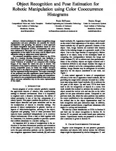
(b) pose estimation. A subset of the cars was annotated with one of 40 different labels corresponding to approximately uniform samples of the azimuth range. We show our label differences alongside those reported in [1].
Figure 5. 3D-pose cars - pose estimation. A confusion matrix and a histogram of label differences. Average accuracy is 85.28%.
Figure 4. Pascal VOC 2007 cars.
AP AA
voting 90.17%
voting + SVM 94.85% 83.88%
voting + 8view-SVM 99.16% 85.28%
Table 2. Results on 3D-pose cars. Average Precision (AP) and Average Accuracy (AA) for pose estimation.
different elevations. We follow [20], and use sets 1-5 for training and sets 6-10 for testing. We train an SVM using sets 1-5 along with positive examples from our own dataset, negative examples are taken from Pascal. AP scores were computed using the Pascal VOC2010 evaluation protocol and are summarized in Table 2. The combination of 3D voting and an 8-view SVM produces an AP result of 99.16% this is an improvement over the previous state-of-the-art (to the best of our knowledge) of 89.8% reported in [20]. Note that [20] use different training data, they rely on 41 car CAD models while we rely on our dataset of 22 cars. We also achieve state-of-the-art results for pose classification on this dataset. Our average classification accuracy results are given in Table 2. Our best result of 85.28% is an improvement over 81% of [20]. Note that [20] report their average accuracy score of 81% on a smaller set (AP = 81.3%) while we achieve a better classification accuracy score on a larger set (AP = 99.16%). A confusion matrix and label differences are presented in Figure 5. Pose estimation on Pascal The Pascal data includes only coarse pose labels (frontal / rear / right / left). ArieNachimson and Basri [1] augmented the pose labels on a subset of the 2007 test category. They labeled approximately 200 car instances with one of 40 labels which correspond to an approximately uniform sample of azimuth an-
(a) EPFL multiview cars - pose (b) Our car dataset - pose estimaestimation. A histogram of the an- tion. We achieve a median angular gular errors in pose estimates. Our error of 10.4 degrees. median angular error is 24.83 degrees. Computed on an 89.54% AP detection set.
Figure 6. Pose estimation results.
gles. In their paper they report differences between the labels of their estimated pose and the ground truth labels for 188 objects. We detected 180 of these objects, and compared our pose estimation to theirs in Figure 4(b). EPFL car data set The EPFL multiview car dataset was introduced in [17]. The dataset was acquired at a car show, 20 different models were imaged every 3 to 4 degree while the cars were rotating to produce a total of approximately 2000 images. We train 8-view SVM classifiers using the positive examples from the first 10 models along with images from our dataset and from the 3D-pose dataset. Negative examples were taken from Pascal training images. We ran our 3D-voting followed by SVM on the last 10 models achieving an average precision of 89.54% (measured using Pascal VOC 2010 evaluation protocol). We then evaluate our pose estimates on the true detections. We achieve a median angular error of 24.83 degrees. We show a histogram of the angular errors in our pose estimates in Figure 6(a). [17] shows a similar histogram, however our results are not directly comparable since they report pose estimates on all of the windows which were considered by their classifier and overlapped the ground truth by more than one half.
Pose estimation on our car dataset We conclude with a pose estimation experiment on our car dataset. We partition the 22 cars into three sets of size 7,7 and 8 and run three experiments in which we use one set for testing and the other two to generate our 3D model and 3D voting detector. We then take the top-scoring detection from each image. In some of the images the top scoring detection is a car in the background of the image. We discard these detections and evaluate pose on the remaining detections in which the pose annotated car was detected. We achieve fairly accurate pose estimation with a median angular error of 10.4 degrees. A histogram of angular errors is shown in Figure 6(b).
6. Conclusions In this paper we have described an approach that handles detection and viewpoint estimation as a joint task, and integrates reasoning about appearance and shape of the objects in a “native” way. Along the way we have made a number of choices that stand in contrast to related work in the literature. One is the construction of a nonparametric model, which maintains multiple instances of objects and multiple features without quantization or clustering. Another is to reason about detection and viewpoint jointly in a 6D parameter space, and to parametrize hypotheses in this space by means of projecting a set of designated points. Finally, we use the viewpoint estimate provided by the voting method to apply viewpoint-aware verification and refinement mechanism. We believe that these choices all serve to improve performance of the detector, as demonstrated in our experiments. In the current system each vote counts equally. We believe that one can improve performance significantly by discriminatively learning weights to be assigned to 3D features; such an extension is the subject of our current work.
References [1] M. Arie-Nachimson and R. Basri. Constructing implicit 3d shape models for pose estimation. In ICCV, 2009. 2, 7 [2] O. Boiman, E. Shechtman, and M. Irani. In defense of nearest-neighbor based image classification. In CVPR, 2008. 2 [3] L. Bourdev, S. Maji, T. Brox, and J. Malik. Detecting people using mutually consistent poselet activations. In ECCV, 2010. 2 [4] M. Everingham, L. Van Gool, C. K. I. Williams, J. Winn, and A. Zisserman. The pascal visual object classes (voc) challenge. IJCV, 88(2), 2010. 6 [5] P. Felzenszwalb, R. Girshick, D. McAllester, and D. Ramanan. Object detection with discriminatively trained part based models. PAMI, 2010. 4 [6] P. Felzenszwalb, D. McAllester, and D. Ramanan. A discriminatively trained, multiscale, deformable part model. In CVPR, 2008. 2, 4
[7] M. Fischler and R. Bolles. Random sample consensus: a paradigm for model fitting with application to image analysis and automated cartography. Communications of the ACM, 24(6), 1981. 1 [8] Y. Furukawa and J. Ponce. Accurate, dense, and robust multiview stereopsis. PAMI, 2010. 1, 5 [9] D. Glasner and G. Shakhnarovich. Nonparametric voting architecture for object detection. TTIC Technical Report, (1), 2011. 5 [10] C. Gu and X. Ren. Discriminative Mixture-of-Templates for Viewpoint Classification. In ECCV, 2010. 2 [11] W. Hu and S. Zhu. Learning a Probabilistic Model Mixing 3D and 2D Primitives for View Invariant Object Recognition. In CVPR, 2010. 2 [12] B. Leibe, A. Leonardis, and B. Schiele. Robust object detection with interleaved categorization and segmentation. IJCV, 2008. 2 [13] Y. Li, L. Gu, and T. Kanade. A robust shape model for multiview car alignment. In CVPR, June 2009. 2 [14] J. Liebelt and C. Schmid. Multi-view object class detection with a 3d geometric model. In CVPR, 2010. 2 [15] J. Liebelt, C. Schmid, and K. Schertler. Viewpointindependent object class detection using 3D feature maps. In CVPR, 2008. 2 [16] D. Mount and S. Arya. ANN library. www.cs.umd.edu/˜mount/ANN. 5 [17] M. Ozuysal, V. Lepetit, and P. Fua. Pose estimation for category specific multiview object localization. In CVPR, 2009. 1, 2, 6, 7 [18] S. Savarese and L. Fei-Fei. 3D generic object categorization, localization and pose estimation. In ICCV, 2007. 1, 2, 6 [19] N. Snavely, S. M. Seitz, and R. Szeliski. Photo Tourism: Exploring Image Collections in 3D. In ACM Transactions on Graphics (Proceedings of SIGGRAPH 2006), 2006. 1, 5 [20] M. Stark, M. Goesele, and B. Schiele. Back to the future: Learning shape models from 3d cad data. In BMVC, 2010. 2, 7 [21] H. Su, M. Sun, L. Fei-Fei, and S. Savarese. Learning a dense multi-view representation for detection, viewpoint classification and synthesis of object categories. In ICCV, 2009. 2 [22] M. Sun, G. Bradski, B. Xu, and S. Savarese. Depth-Encoded Hough Voting for Joint Object Detection and Shape Recovery. ECCV, 2010. 2, 6 [23] M. Sun, G. Bradsky, B. Xu, and S. Savarese. Depth-encoded hough voting for joint object detection and shape recovery. In ECCV, 2010. 2 [24] M. Sun, H. Su, S. Savarese, and L. Fei-Fei. A Multi-View Probabilistic Model for 3D Object Classes. In CVPR, 2009. 2 [25] A. Thomas, V. Ferrar, B. Leibe, T. Tuytelaars, B. Schiel, and L. Van Gool. Towards multi-view object class detection. In CVPR, volume 2, 2006. 2 [26] A. Vedaldi, V. Gulshan, M. Varma, and A. Zisserman. Multiple kernels for object detection. In ICCV, 2009. 5 [27] Z. Zhang. A flexible new technique for camera calibration. PAMI, 2002. 4