The Least Choice First (LCF) Scheduling Method for High-speed Network Switches
Nils Gura and Hans Eberle
The Least Choice First (LCF) Scheduling Method for High-speed Network Switches
Nils Gura and Hans Eberle
SMLI TR-2002-116
October 2002
Abstract: We describe a novel method for scheduling high-speed network switches. The targeted architecture is an input-buffered switch with a non-blocking switch fabric. The input buffers are organized as virtual output queues to avoid head-of-line blocking. The task of the scheduler is to decide when the input ports can forward packets from the virtual output queues to the corresponding output ports. Our Least Choice First (LCF) scheduling method selects the input and output ports to be matched by prioritizing the input ports according to the number of virtual output queues that contain packets: The fewer virtual output queues with packets, the higher the scheduling priority of the input port. This way, the number of switch connections and, with it, switch throughput is maximized. Fairness is provided through the addition of a round-robin algorithm. We present two alternative implementations: A central implementation intended for narrow switches and a distributed implementation based on an iterative algorithm intended for wide switches. The simulation results show that the LCF scheduler outperforms other scheduling methods such as the parallel iterative matcher [1], iSLIP [12], and the wave front arbiter [16]. This report is an extended version of a paper presented at IPDPS 2002, Fort Lauderdale, Florida, April 2002.
M/S MTV29-01 2600 Casey Avenue Mountain View, CA 94043
email address:
[email protected] [email protected]
© 2002 Sun Microsystems, Inc. and The Institute of Electrical and Electronics Engineers, Inc. All rights reserved. The SML Technical Report Series is published by Sun Microsystems Laboratories, of Sun Microsystems, Inc. Printed in U.S.A. Unlimited copying without fee is permitted provided that the copies are not made nor distributed for direct commercial advantage, and credit to the source is given. Otherwise, no part of this work covered by copyright hereon may be reproduced in any form or by any means graphic, electronic, or mechanical, including photocopying, recording, taping, or storage in an information retrieval system, without the prior written permission of the copyright owner. TRADEMARKS Sun, Sun Microsystems, the Sun logo, and Java are trademarks or registered trademarks of Sun Microsystems, Inc. in the U.S. and other countries. For information regarding the SML Technical Report Series, contact Jeanie Treichel, Editor-in-Chief . All technical reports are available online on our Website, http://research.sun.com/techrep/.
The Least Choice First (LCF) Scheduling Method for High-speed Network Switches Nils Gura and Hans Eberle Sun Microsystems Laboratories 2600 Casey Avenue Mountain View, CA 94043 {nils.gura,hans.eberle}@sun.com
1. Introduction The switch scheduling problem described here is an application of bipartite matching on a graph with 2⋅n vertices: Each one of the n output ports has to be matched, that is, connected with at most one of the n input ports that has packets to be forwarded. There are algorithms known as maximum size matching that find the most number of matches and, applied to the switch scheduling problem, find a schedule that maximizes switch throughput.1 Unfortunately, these algorithms are too slow for applications in high-speed networking and lead to starvation [9]. When designing a switch scheduler the following criteria have to be considered: • Throughput: Switch bandwidth is a valuable resource that has to be utilized as efficiently as possible. Poor utilization of the switch leads to poor utilization of the attached links and the remainder of the network. • Fairness: Starvation is to be avoided by guaranteeing a minimum level of fairness so that progress is being made. When examining scheduling algorithms, fairness is often cited without giving a clear definition. Here, we define fairness as the lower bound on the fraction of output link bandwidth allocated to each input port. • Latency: Packet switching networks running at Gbit/s line rates that switch packets at high rates require high-speed scheduling algorithms. Timing requirements can be relaxed with the help of pipelining techniques. By pipelining the scheduler and overlapping scheduling and packet forwarding, packet throughput is optimized. Note that these techniques do not reduce latency and that the scheduling latency adds to the overall switch forwarding latency. • Cost: The cost of an implementation is determined by the amount of real estate used on chips and boards, and by the pin count of chips and board connectors. An important cost factor is the amount of signal wires needed to communicate scheduling information. • Modularization: The topology of the communication paths needed between scheduler and switch ports impacts modularization of the switch implementation. • Scalability: An implementation of a scheduling algorithm ideally scales to a large number of switch ports. A measure of scalability is the O-notation that characterizes the complexity of an algorithm in respect to execution time and implementation size.
1
Maximum size matching does not necessarily guarantee that throughput is optimized over time.
1
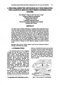
It is important to note that some of the criteria listed above cannot be optimized at the same time. In particular, throughput has to be traded off against fairness, latency, and scalability. High throughput is only achieved at the cost of fairness as it can be easily shown that an algorithm that finds the maximum number of matches can lead to starvation. Further, high throughput usually implies high latency since it takes time to optimize a schedule. And finally, scalability can impact throughput as a distributed implementation, rather than a central implementation, is typically needed that requires decisions to be made based on partial rather than global knowledge. Considering the tradeoff between throughput and fairness, the LCF scheduler is a hybrid design that uses one algorithm to optimize throughput and another algorithm to provide fairness. Further, we address the tradeoff between throughput and scalability by providing two alternative designs: A central scheduler targeted at narrow switches and a distributed scheduler targeted at wide switches. As we will show, the central scheduler performs slightly better while the distributed scheduler scales better. We have implemented the LCF scheduler as part of the Clint 2 project [4][5][7]. The LCF scheduler is used to schedule a 16-port crossbar switch with an aggregate throughput of 32 Gbit/s. The switch is re-scheduled every 8.5 µs and the actual scheduling time is 1.3 µs. A central implementation of the LCF scheduler was chosen using field-programmable gate array (FPGA) technology. Related Work Surveys of scheduling algorithms are found in [6][11]. Here we want to mention the Parallel Iterative Matcher (PIM) [1] since it has similarities with the distributed version of the LCF scheduler in that it also takes an iterative approach. The difference is the criteria that determines which request to choose. PIM uses randomness while the LCF scheduler uses priorities based on the number of requests and grants. Algorithms similar to PIM have been proposed that use priorities rather than randomness to choose requests and grants: The scheme proposed in [8] uses priority lists and the iSLIP algorithm described in [12] uses rotating priorities to make the necessary choices. Thus, there are similarities with the round-robin algorithm used by the LCF scheduler. The advantage of using a round-robin algorithm is that there is an upper bound on the time it takes to grant a request. The wave front arbiter is a distributed algorithm that maps to an implementation based on a regular array of cells matching the structure of a crosspoint switch [16]. Despite its simplicity the algorithm produces fairly good schedules. Since it is based on a round-robin algorithm, starvation is prevented. 2. Switch Scheduling Problem This section describes the scheduling problem to be solved. More specifically, we describe a switch model to which the scheduling problem applies. Figure 1 shows the switch under consideration. In this example, a crossbar switch with n = 4 ports constitutes the switch fabric. Initiators Ii (0 ≤ i ≤ n-1) and targets Ti (0 ≤ i ≤ n-1) stand for the producers and consumers, respectively, of the packets forwarded by the fabric. Packets are buffered at the input side of the switch. Each input buffer contains one virtual output queue per output port [15] to avoid head-of-line blocking [10]. That is, packets are sorted based on the output port they are destined for when they arrive at the input port and before they are forwarded through the switch fabric. The virtual 2
Clint is the code name of a Sun Microsystems Laboratories internal project.
2
Switch Fabric to T0
I0
to T1
b
b
b
b
b
b
to T2
T0
to T3 to T0
I1
to T1 to T2
T1
to T3 to T0
I2
to T1
T2
to T2 to T3 to T0
I3
to T1
b
b
to T2
T3
to T3
Figure 1: Model of a switch with virtual output queues.
output queues may be served in any order, that is, no ordering rules are imposed when forwarding packets destined for different targets. The scheduler has knowledge of all queues that contain packets to be forwarded. More specifically, the scheduler receives a request vector from each initiator whereby a vector bit indicates whether a virtual output queue contains packets or not. Throughout this paper we assume that there is an equal number n of input and output ports. As a consequence, there are n virtual output queues though implementations might choose n-1 queues if an initiator is assumed not to send packets to itself. Bandwidths of the input and output ports, as well as of the internal paths are identical. That is, output ports receive packets from the input ports at the same rate packets are forwarded to the output link. We are going to use the following notation. A scheduler takes requests for resources from requesters and calculates a conflict-free schedule allocating resources to requesters. Here, the requesters are the input ports of the switch fabric and the resources are the output ports of the switch fabric. Due to the close coupling, we also refer to the initiator connected to the input port as the requester and to the target connected to the output port as the resource. The outlined switch organization with its input buffers is attractive for several reasons. Alternative designs such as shared memory switches [14][3] or output-buffered switches do not scale to higher speeds and larger port numbers as well as input-buffered switches. This is explained by the different bandwidth requirements of the buffer memory: For a shared memory switch, the read and write bandwidth is n⋅b where n is the number of ports and b is the bandwidth per link; for an input buffer, the read and write bandwidths are b; and for an output buffer, the read bandwidth is b and the write bandwidth is n⋅b. We assume a non-blocking switch fabric such as the crossbar switch of Figure 1. Other nonblocking fabrics such as Clos networks are also possible [2].
3
1 2 3 4 5 6 7 8 9 10 11 12 13 14 15 16 17 18 19 20 21 22 23 24 25 26 27 28 29 30 31 32 33 34 35 36 37
var I: 0..MaxReq-1; (* current round-robin requester offset *) J: 0..MaxRes-1; (* current round-robin resource offset *) req: 0..MaxReq-1; (* requester *) res, r: 0..MaxRes-1; (* resource *) gnt: -1..MaxReq-1; (* granted request *) min: 0..MaxRes+1; (* minimum number of requests *) R: array [0..MaxReq-1, 0..MaxRes-1] of boolean; (* R[i,j]: requester i requesting resource j *) nrq: array [0..MaxReq-1] of 0..MaxRes; (* number of resources requested by a requester *) S: array [0..MaxReq-1] of -1..MaxRes; (* S[i] contains the granted request for requester i; *) (* if it contains -1, no request was granted *) procedure schedule; begin for req := 0 to MaxReq-1 do S[req] := -1; (* initialize schedule *) nrq[req] := 0; for res := 0 to MaxRes-1 do if R[req,res] then nrq[req] := nrq[req]+1; (* calculate number of requests for each requester *) for res := 0 to MaxRes-1 do (* allocate resources one after the other *) gnt := -1; if R[(I+res) mod MaxReq,(J+res) mod MaxRes] then gnt := (I+res) mod MaxReq (* round-robin position wins *) else (* find requester with smallest number of requests *) min := MaxRes+1; for req := 0 to MaxReq-1 do if (R[(req+I+res) mod MaxReq,(res+J) mod MaxRes]) and (nrq[(req+I+res) mod MaxReq] < min) then gnt := (req+I+res) mod MaxReq; min := nrq[(req+I+res) mod MaxReq]; if gnt -1 then S[gnt] := (res+J) mod MaxRes; for r := 0 to MaxRes-1 do R[gnt, r] := false; nrq[gnt] := 0; for req := 0 to MaxReq-1 do if R[req, (res+J) mod MaxRes] then nrq[req] := nrq[req]-1; I := (I+1) mod MaxReq; if I = 0 then J := (J+1) mod MaxRes; end;
Figure 2: Pseudo code describing the central LCF scheduler.
Packets have a fixed size and connections between input and output ports are scheduled in discrete time steps or slots that are aligned in the sense that initiators start and stop packet transmission simultaneously. Fixed-size packets offer the advantage of simpler switch scheduling and buffer management. Also, they make the scheduling of traffic with real-time demands easier. The scheduler’s task is to calculate a schedule for each slot that determines the connections between input and output ports. For this purpose, it has to examine n2 requests as each one of the n initiators can have up to n requests. The schedule has to be conflict-free and is typically optimized such that maximum switch throughput is achieved while some minimum level of fairness is still maintained. 3. The Central LCF Scheduler The LCF scheduler selects the requests to be granted by prioritizing the initiators based on the number of targets they request. The priorities are calculated as the inverse of the number of targets an initiator is requesting, that is, the fewer requests an initiator has, the higher its priority. This rule can be explained as follows. An initiator with many requests has many choices and an initiator with few requests has few choices. To optimize the total number of granted requests, the high-priority initiators with few requests are scheduled before the low-priority initiators with many requests are scheduled. To avoid starvation, we added a round-robin scheme that is interleaved with the operation of the LCF scheduler. The pseudo code for the LCF scheduler is shown in Figure 2.
4
1) T0 T1 T2 T3 NRQ
2) T0 T1 T2 T3 NRQ
I0 0
1
1
0 2
I0
I1 1
0
1
1 3
I1
1
1
0 2
I2 1
0
1
1 3
I2
0
1
1
I3 0
1
0
0 1
I3
1
0
0 1
2
3) T0 T1 T2 T3 NRQ
4) T0 T1 T2 T3 NRQ
I0
I0
1
0 1
I1 I2
I1 1
I2
1 2
I3
1
1
I3 round-robin position granted request scheduled resource
Figure 3: Example of a LCF scheduling cycle.
To describe the scheduling scheme in detail, we consider a 4x4 switch. In the example shown in Figure 3, initiator I0 requests targets T1 and T2; initiator I1 requests targets T0, T2 and T3; initiator I2 requests targets T0, T2, and T3; and initiator I3 requests target T1. Column NRQ shows the number of requests for each requester. Targets are scheduled sequentially; in this example, the order is: T0, T1, T2, and T3. This scheduling sequence is rotated periodically so that none of the targets is favored. Each target is scheduled in two steps. First the round-robin position is examined. If there is a request in the round-robin position, it is granted before any other request is considered. If it is not set, the request of the initiator with the highest priority, that is, with the least number of requests is granted. If there are several initiators with the highest priority, a rotating priority chain starting at the round-robin position determines the request to be granted. The number of requests NRQ and, with it, the priorities are recalculated when a new target is scheduled so that only requests for targets that have not been scheduled are considered. As shown, the round-robin positions form a diagonal which covers positions [I1, T0], [I2, T1], [I3, T2], and [I0, T3]. The diagonal moves every scheduling cycle. Its starting position [Ii, Tj] is calculated as follows: i := (i+1) mod n; if i=0 then j := (j+1) mod n. This way, every position in the matrix is given the highest priority every n2 scheduling cycles. In the example of Figure 3, T0 is scheduled first. The round-robin position favors I1 and its request is, therefore, granted. Next, T1 is scheduled. There are requests for this target by I0 and I3. Since I3 has higher priority, its request is granted. When scheduling T2 there is choice between the requests by I0 and I2. In this case, I0 has higher priority and, so, its request is granted. Finally, T3 is scheduled. There is no choice and the request by I2 is granted. There is a tradeoff to be made between throughput and fairness. Optimizing a scheduler for throughput affects fairness adversely and leads to starvation. This can be illustrated with the example of Figure 3. If we want to optimize bandwidth utilization, we can either grant [I1, T0], [I3, T1], [I0, T2], [I2, T3] or [I2, T0], [I3, T1], [I0, T2], [I1, T3]. This is unfair as requests [I0, T1], [I1, T2], [I2, T2] are ignored. They are ignored since only three requests rather than four requests could be granted. The addition of the round-robin scheduler avoids starvation in that every request [Ii, Tj] is periodically visited and granted. Variations of the round-robin scheduler are possible in that a
5
SendBuffers bini0
bini1
1
Bulk Switch 1
RecvBuffers 1
btgt0
1
1
1
btgt1
Bulk Scheduler
qini0
qini1
1
8
1
1
8
1
qtgt0
qtgt1
Quick Switch
Figure 4: Organization of the Clint switch.
single position, a row or column are covered every scheduling cycle. Unlike other algorithms such as the PIM, the scheduler described here guarantees a lower bound on the fraction of bandwidth of a target each virtual output queue receives. For the algorithm shown in Figure 2, this fraction is b/n2 with b being the bandwidth available per port. The algorithm can be easily changed to decrease or increase this fraction in the range 0..b/n. The lower bound of this range is given by a pure LCF scheduler and the upper bound is given by a scheduler that uses a diagonal of round-robin positions all of which are scheduled before any other position is considered. 4. The Clint Implementation We have implemented an LCF scheduler for the cluster interconnect Clint [4][5]. Figure 4 shows the organization of Clint. Clint is characterized by a segregated architecture that provides two physically separate transmission channels: A bulk channel optimized for high-bandwidth traffic and a quick channel optimized for low-latency traffic. Each channel uses its own switch and links. Different scheduling strategies are applied to the two channels. The bulk channel uses an LCF scheduler that allocates time slots on the transmission paths before packets are sent off. This way collisions are avoided that lead to blockages and, with it, performance loss. In contrast, the quick channel takes a best-effort approach and packets are sent whenever they are available. If they collide in the switch, one packet wins and is forwarded while the other packets are dropped. The current Clint prototype implements a star topology using a single switch that supports up to 16 host computers. In this section we describe the implementation of the LCF scheduler used for the bulk channel. We begin with a description of the communication protocol. Next, we describe the hardware implementation of the scheduler. Finally, we describe an extension of the scheduler that uses a precalculated schedule intended for forwarding real-time traffic as well as multicast traffic.
6
c
c+1 n
n-1
bini0
breq0,1
bini1
breq1,0
c+2 n+1
breq0,
breq0,1 n
n-1
n+1
breq1,
breq1,0
qini0 n
cfg0,s
n+1
n
gnts,0
cfg0,s
n+1
n
n+1
n
gnts,0 back1,0
qini1 n
cfg1,s
n+1
n
gnts,1
cfg1,s
gnts,1 back0,1
Figure 5: Channel timing.
4.1. Communication Protocol Data transmission follows a request-acknowledgment protocol whereby the payload containing the data is always part of the request packet and an acknowledgment packet is returned for the receipt of every request packet. While only bulk requests use the bulk channel, all other packets including bulk acknowledgments, quick requests and quick acknowledgments use the quick channel. In addition, the quick channel is used for the exchange of information between the hosts and the bulk scheduler. Two packet formats are introduced to deliver this information: • The configuration packets are sent from the hosts to the switch and contain the following fields: {type=cfg | req[15..0] | pre[15..0] | ben[15..0] | qen[15..0] | CRC[15..0]}. req specifies the requested targets; pre is the precalculated schedule explained in Section 4.3; ben and qen specify the bulk initiators and quick initiators, respectively, from which packets are to be forwarded by the switch – hosts use these fields to disable malfunctioning hosts; CRC is the checksum used to detect transmission errors. • The grant packets are sent from the switch to the hosts and contain the following fields: {type=gnt | nodeId[3..0] | gnt[3..0] | gntVal | linkErr | CRCErr | CRC [15..0]}. nodeId is used at initialization time to assign a unique id to the receiving host; gnt contains the encoded target number of the granted request; gntVal says whether gnt is valid; linkErr is set if a link error was detected since the last grant packet was sent; CRCErr is set if the last configuration packet had a CRC error or was missing. The bulk channel corresponds to a pipeline consisting of three stages: During the scheduling stage, configuration and grant packets are exchanged between the hosts and the switch to schedule the bulk switch; during the transfer stage, bulk request packets are transferred between initiators and targets; during the acknowledgment stage, acknowledgment packets are returned from the targets to the initiators. Figure 5 shows an example with two pairs of initiators bini and qini that generate packets for the bulk and quick channel, respectively. The stages of the bulk pipeline can be easily identified. Looking at the transfer of bulk request packet breqn0,1 slot c corresponds to the scheduling stage, slot c+1 to the transfer stage, and slot c+2 to the acknowledgment stage. The sequence of packets is as follows. In slot c, configuration packets cfgn0,s and cfgn1,s are sent
7
+1 RES
R[0,*]
res_inc
n
… 0
…
n-1
sum nrq_set
CP
NGT
shift_ prio
PRIO
NRQ 0 1
gnt_set
nrq_en
prior_ en
GNT
0
0 …
…
n …
Figure 6: Block diagram of the LCF scheduler implementation.
from bini0 and bini1, respectively, to the switch. The scheduler calculates the schedule and returns the results in grant packets gntns,0 and gntns,1: bini0 is granted the request for btgt1 and bini1 is granted the request for btgt0. In slot c+1, the corresponding request packets breqn0,1 and breqn1,0 are transferred. Finally, in slot c+2, the acknowledgment packets are transferred, that is, btgt0 sends backn0,1 to bini1 and btgt1 sends backn1,0 to bini0. 4.2. Hardware Description Figure 6 describes the hardware implementation of the central LCF scheduler. Shown is the logic associated with requester 0. Requesters may be spatially separated and use an n-bit open collector bus to compare their priorities. Request register R[0,0..n-1] is an n-bit vector with the requests; it corresponds to the first row of the request matrix shown in Figure 3. Before a resource is scheduled, requesters sum up their requests and store the results in register NRQ. They also set their NGT flags to indicate that they have not yet received a grant. NRQ is implemented as an n-bit shift register containing the number of requests in inverse unary encoding. For example, to represent three requests, NRQ is set to 1…1000. Using this representation, decrementing the number of requests by one can be efficiently done by a shift operation. Resource register RES points to the next resource to be scheduled. Scheduling of a resource is done as follows. Requesters with requests place the content of NRQ onto the bus whereby NGT ensures that only requesters participate that have not yet been granted a resource. Higher NRQ values indicating lower priorities are overwritten with lower NRQ values. If, for example, one requester has three requests and another has one request, vectors 0…0111 and 0…0001, respectively, are written to the bus. Sampling the bus, 0…0001 will be seen. By comparing NRQ with the value seen on the
8
1) T0 T1 T2 T3 NRQ
2) T0 T1 T2 T3 NRQ
I0 1
0
1
I0
I1 1
1
2
I1
I2 1
1
2
I2
0
0 1
1
I3
I3
precalculated schedule round-robin position granted request scheduled resource Figure 7: Example of a precalculated multicast connection.
bus, requesters determine whether they had the highest priority and, if so, set their CP flag. To arbitrate among multiple requesters with the same number of requests, requesters output the priority stored in PRIO to the bus in the next scheduling step. Shift registers PRIO contain a unique priority for each requester in inverse unary encoding. Together with the open collector bus, they form a programmable priority encoder as suggested in [12]. If a requester determines that it has the highest priority, it sets its GNT register to the value in RES which corresponds to the resource that is currently being scheduled. Priorities are rotated every scheduling cycle. Round robin positions are implemented simply by having the requester with the highest priority participate in the second step independent of its number of requests. Prior to scheduling a resource, registers PRIO are shifted to rotate the priorities of the requesters, registers NRQ are updated to reflect the outstanding numbers of requests and resource pointers RES are incremented to point to the next resource. By shifting PRIO one more time after completing a schedule and incrementing RES an additional time after n scheduling cycles, scheduling starts with different round-robin positions and considers different resources first. Thus, fairness and bandwidth guarantees can be provided. For n resources, 2n+1 cycles are needed to execute the LCF algorithm. 4.3. The Precalculated Schedule Clint implements a precalculated schedule which allows initiators to pre-schedule requests prior to the regular scheduling operation. The precalculated schedule is intended to be used for scheduling real-time traffic or multicast packets. The precalculated schedule is communicated to the LCF scheduler as part of the configuration packet. An example is shown in Figure 7. In this example a multicast connection has been precalculated between I3 and T1 and T3. How they calculate the precalculated schedule, is up to the initiators. While it is assumed that the precalculated schedule is conflict-free, the LCF scheduler checks the integrity of the schedule. Scheduling happens in two stages. In the first stage, the integrity of the precalculated schedule is checked. The integrity is violated if there are multiple requests for a target. In such a case, one request is accepted and the remaining ones are dropped. In the second stage, the LCF
9
I0
T0
I0
T0
I1
T1
I1
T1
. . .
. . .
. . .
. . .
In-1
Tn-1
In-1
Tn-1
Distr. Sched.0 Distr. Sched.1
Distr. Sched.n-1
Central Scheduler
(b)
(a)
Figure 8: Central scheduler (a) vs. distributed scheduler (b).
scheduler does its regular work. The precalculated schedule does not add any overhead in the sense that the existing logic of the LCF scheduler is used during the first stage. Note that the precalculated schedule can cause conflicts with the round-robin positions and, thus, impact fairness. 5. The Distributed LCF Scheduler As shown in Figure 8, we can distinguish between central and distributed scheduler implementations. A central scheduler collects the requests in a central location, where it calculates a schedule, typically by making use of the global knowledge it has about requests and grants. In contrast, a distributed scheme splits the necessary scheduling logic into several distributed schedulers such that each resource is scheduled by its local scheduler that operates without global knowledge of the requests and grants. Comparing the performance of the two alternatives, scalability comes at a price: The central scheduler can calculate a more efficient schedule thanks to global knowledge while the distributed scheduler scales to a larger number of switch ports. So far we have considered a central implementation of the LCF scheduler. A distributed version similar to the iterative approach of the PIM [1] is also possible. Scheduling is done in several rounds or iterations each of which consists of three steps: • Request: Each unconnected or unmatched initiator sends a request to every target for which it has a packet. The request is accompanied by a priority which is given by the number of requests the initiator is sending — the fewer requests being sent, the higher the priority. • Grant: If an unmatched target receives any requests, it grants the one accompanied by the highest priority. If more than one request has the highest priority, a round-robin algorithm is used to select the request to be granted. The grant sent from the target to the initiator is accompanied by a priority which is given by the number of requests the target is receiving — the fewer requests the target is receiving, the higher the priority.
10
Iteration 0
Request
Grant
NRQ 1 I0
T0
3
I1
3 2
Accept
I0
NGT T0 1
I0
T0
T1
I1
T1
2
I1
T1
I2
T2
I2
T2
3
I2
T2
I3
T3
I3
T3
3
I3
T3
Request
Grant
Accept
Iteration 1
NRQ
3
NGT I0
T0
I0
T0
I0
T0
I1
T1
I1
T1
I1
T1
I2
T2
I2
T2
I2
T2
I3
T3
I3
T3
I3
T3
1
Figure 9: Two iterations of the distributed scheduler.
•
Accept: If an unmatched initiator receives any grants, it accepts the one accompanied by the highest priority. If more than one grant has the highest priority, a round-robin algorithm is used to select the grant to be accepted.
During an iteration, only unmatched initiators and targets are considered. As will be shown in Section 6.2, a small number of iterations is normally sufficient to find a near-optimal schedule. Figure 9 gives an example of a schedule calculated for a 4x4 switch in two iterations. It illustrates how choices are made based on the number of requests NRQ and the number of grants NGT, respectively. For example, looking at the request step of iteration 0, T2 receives requests from I0, I1, and I2. With one request (NRQ=1), I0 has the highest priority and, therefore, receives a grant. And looking at the grant step of iteration 0, I3 receives grants from T1 and T3, and accepts the grant from T1 since it has the higher priority (NGT=2 for T1 and NGT=3 for T3). Again, we have added a round-robin algorithm to guarantee fairness. For every scheduling cycle, one element of the request matrix shown in Figure 3 is the round-robin position that is given the highest priority in that it is scheduled before regular LCF scheduling takes place. 6. Evaluation In this section, we first quantify the implementation cost of the LCF scheduler in terms of gate count and execution time. Next, we compare implementations of the central and distributed versions of the LCF scheduler. And finally, we present queuing delays simulated for the LCF scheduler and other well-known schedulers. 6.1. Implementation Cost We have implemented a central LCF scheduler for a 16-port switch in a Xilinx XCV600 FPGA [17]. As we had shown in Figure 6, the implementation is partitioned such that the scheduler logic can be located next to the input ports. Table 1 gives the gate and register counts for this
11
implementation – a gate refers to a two-input gate. Separate counts are shown for the distributed and central parts of the logic. Table 1: Gate count and register count for the LCF scheduler.
Gate count Register count
Distributed 16x450=7200 16x86=1376
Central 767 216
Total 7967 1592
The stated numbers correspond to 15% of the available FPGA resources. Though the implementation of both the quick switch and the bulk scheduler uses a total of 50% of the FPGA’s logic resources, the routing resources are almost fully utilized. Next, the timing of the implemented LCF scheduler is examined. Table 2 lists the tasks of the LCF scheduler and the number of clock cycles taken to execute them. The clock frequency is 66 MHz. Table 2: Scheduling tasks.
Task Check precalculated schedule Calculate LCF schedule Total
Decomposition 2n+1 3n+2 5n+3
Clock Cycles 33 50 83
Time 500 ns 758 ns 1258 ns
6.2. Central vs. Distributed LCF Scheduler In this section, we characterize and compare implementations of the central and distributed scheduler. Speed The time complexity for the central scheduler is O(n) since targets are scheduled sequentially assuming it takes one time step to schedule a target. Given the similarity with the PIM, the time complexity for the distributed scheduler is O(log2n) assuming it takes one time step for each iteration. Obviously, the distributed version is considerably faster than the central scheduler for large values of n. Communication Cost Figure 10 shows the exchanges of messages required for a central and a distributed implementation of the LCF scheduler. Other ways to encode the messages are, of course, possible.
12
I0
req(n) gnt(log2n), vld(1)
I1
req(n) gnt(log2n), vld(1)
Central Sched.
(a)
I0
req(1),nrq(log 2n) gnt(1),ngt(log2n ) acc(1)
I1 (b)
Distr. Sched.0
Distr. Sched.1
Figure 10: Communication required for the central scheduler (a) and the distributed scheduler (b).
The central scheduler receives and sends a total of n(n+log2n+1) bits. The collection of scheduler slices making up the distributed scheduler exchange a total of i⋅n2(2⋅log2n+3) bits, where i stands for the number of iterations. Comparing the two schemes, the distributed scheduler has significantly higher communication demands since the priorities have to be explicitly sent, and, possibly, have to be sent to multiple resources. That is, the priorities of the requests given by the number of requests nrq have to be sent to every requested resource. And similarly, the priorities of the resources given by the number of received requests ngt have to be sent to every requester. Of course, if busses are used instead of point-to-point connections for transmitting nrq and ngt, bandwidth is saved. Modularization The choice of the scheduler affects the modularization of the implementation. Typically, a switch implementation modularizes the design such that there is a backplane holding the switching fabric and line cards containing the logic associated with the input and output ports. Separating these two types of cards results in higher flexibility as line cards can be added as needed and different types of line cards interfacing different types of links can be plugged into the same backplane. The outlined physical structure calls for the central scheduler to be packaged together with the switching fabric and for the distributed scheduler to be packaged together with the line cards. The latter approach is particularly interesting when a scalable design is considered that uses a bit-sliced switch fabric. 6.3. Performance Simulation Results We have simulated the LCF scheduler and other scheduling methods with the help of the simulation model shown in Figure 11. Packets are generated by packet generators PGs. They are
13
VOQ
Switch Switch Fabric
PQ I0
.. .
PG
T0
.. . VOQ PQ I1
PG
.. .
T1
PG: Packet Generator PQ: Packet Queue VOQ: Virtual Output Queue
Figure 11: Simulation model.
first buffered in the packet queues PQ and next, if space permits, in the virtual output queues VOQ. PQs and VOQs are FIFO memories. Together, PGs and PQs model the initiators injecting packets into the network. The following scheduling methods have been simulated: • fifo: This scheduler uses a single FIFO queue per input port (replacing multiple VOQs). The scheduler serves the FIFO queues in a round-robin fashion. • lcf_central: This is the central LCF scheduler. • lcf_central_rr: This is the central LCF scheduler extended with a round-robin algorithm. The round-robin algorithm uses a round-robin diagonal as described in Figure 2 and 3. • lcf_dist: This is the distributed LCF scheduler. • lcf_dist_rr: This is the distributed LCF scheduler extended with a round-robin algorithm. The round-robin algorithm uses a single round-robin position for each scheduling cycle. • pim: This is the parallel iterative matcher [1]. • islip: This is the iSLIP scheduler [12]. • wfront: This is the wrapped wave front scheduler [16]. • outbuf: This models an output-buffered switch. We first examine simulation results for non-bursty traffic. Figure 12a shows the average queuing delay measured in packet time slots versus load. Load is the probability that a host generates a packet in a given time slot. The destinations of the packets are distributed uniformly. The following parameters were used: The switch has 16 ports; each VOQ has 256 entries and the PQ has 1000 entries; it takes the iterative schedulers pim, lcf_dist, lcf_dist_rr four iterations to cal-
14
culate the schedule; the output buffers of outbuf each contain 256 entries. A buffer or queue entry is large enough to hold a complete packet. Studying the graphs the following observations can be made. The fifo scheduler has the worst performance as it exhibits head-of-line blocking [10]. At the other end of the spectrum is outbuf scheduling, which shows the best performance, since in contrast to the other schedulers, packets are only delayed due to contention for output link bandwidth, and not due to contention for both internal bandwidth as well as output link bandwidth. For low load, the latencies for the various schedulers differ very little. To better illustrate the differences in latency times, we have plotted the same data as latency relative to the latency simulated for output buffering. This is shown in Figure 12b. lcf_central comes closest to the performance of an output-buffered switch except for load above 0.9. It performs significantly better than any other scheduler examined. For high load, the latency for lcf_central is about 1.4 times the latency of outbuf. The latencies for lcf_central_rr are only slightly worse than the latencies for lcf_central up to a load of about 0.9. If the load is further increased, the latencies for lcf_central_rr suddenly become significantly less than the ones obtained for lcf_central. This is probably the case since the round robin algorithm of lcf_central_rr is leveling the lengths of the VOQs thereby maintaining choice by avoiding the VOQs to drain. We observe a similar change in trend for the distributed versions: lcf_dist has lower latencies than lcf_dist_rr up to a load of 0.9; as the load is further increased, the latencies simulated for lcf_dist_rr are staying lower than the ones obtained for lcf_dist. Compared with pim, lcf_dist has lower and lcf_dist_rr higher latencies for a load up to 0.9; beyond this point, lcf_dist has higher and lcf_dist_rr lower latencies. As expected, the distributed schedulers perform slightly worse than a central scheduler such as lcf_central since the distributed schedulers have to work with partial information. islip and wfront seem to be similar in performance probably since in both cases scheduling decisions are based on a round-robin algorithm. Figure 13a and Figure 13b show the average queuing delay and relative latency, respectively, for bursty traffic. The distribution of the burst lengths is uniform with the maximum length being five packets. As expected, bursty traffic increases the latency for all scheduling methods. The graphs, further, show that the latencies measured for the various methods differ less for bursty traffic than for non-bursty traffic.
15
25 lcf_central lcf_central_rr lcf_dist lcf_dist_rr pim islip wfront fifo outbuf
latency [packets]
20
15
10
5
0 0
0.1
0.2
0.3
0.4
0.5
0.6
0.7
0.8
0.9
1
load
Figure 12a: Simulated latencies for non-bursty traffic.
3
lcf_central lcf_central_rr lcf_dist lcf_dist_rr pim islip wfront fifo outbuf
relative latency
2.5
2
1.5
1 0
0.1
0.2
0.3
0.4
0.5 load
0.6
0.7
0.8
0.9
Figure 12b: Simulated relative latencies for non-bursty traffic.
16
1
25
lcf_central lcf_central_rr lcf_dist lcf_dist_rr pim islip wfront fifo outbuf
latency [packets]
20
15
10
5
0 0
0.1
0.2
0.3
0.4
0.5 load
0.6
0.7
0.8
0.9
1
Figure 13a: Simulated latencies for bursty traffic.
3
lcf_central lcf_central_rr lcf_dist lcf_dist_rr pim islip wfront fifo outbuf
relative latemcy
2.5
2
1.5
1 0
0.1
0.2
0.3
0.4
0.5 load
0.6
0.7
0.8
Figure 13b: Simulated relative latencies for bursty traffic.
17
0.9
1
6.4. Fairness As we had mentioned in the introduction, fairness has to be traded off against throughput. Table 3 lists fairness values we calculated for the scheduling methods described in the previous section. The fairness values are given as the lower bound on the fraction of output link bandwidth allocated to each input port. Table 3: Fairness.
Method lcf_central lcf_central_rr lcf_distr lcf_distr_rr pim islip wfront fifo outbuf
Fairness 0 1/n2 0 1/n2 0 1/n 1/n 1/n 1/n
7. Conclusions An input-buffered switch requires a scheduler to determine the connections between input and output ports. While different scheduling methods have similar performance for low loads, we do see significant differences in performance for high loads. In this paper, we have introduced a central and a distributed version of the LCF scheduler. The central version performs significantly better in terms of queuing delay than other schedulers such as the PIM and iSLIP. The distributed version is similar in performance to the parallel iterative matcher, and superior in performance to iSLIP. While high utilization of the switch bandwidth is an important goal when designing a scheduler, other criteria such as fairness, speed, and cost have to be considered as well. Often, these criteria are not independent of each other; in some cases, they have to be traded off against each other. This is true, in particular, when considering throughput and fairness. We have shown that unlike other schedulers such as the PIM, the LCF scheduler makes it possible to give hard (in contrast to statistical) guarantees by a lower bound on the period each request represented by a requester/resource pair is granted. Acknowledgments We thank Nicolas Fugier and Éric Lemoine for reviewing this paper.
18
References [1] [2] [3]
[4] [5]
[6] [7] [8]
[9] [10]
[11] [12] [13] [14] [15]
[16] [17]
T. Anderson, S. Owicki, J. Saxe, C. Thacker: High Speed Switch Scheduling for Local Area Networks. Systems Research Center Report 99, April 26, 1993. C. Clos: A Study of Non-Blocking Switching Networks. The Bell System Technical Journal, vol. 32, 1953, pp. 406-421. H. Eberle, E. Oertli: Switcherland: A QoS Communication Architecture for Workstation Clusters. Proc. ACM 25th Annual International Symposium on Computer Architecture, Barcelona, Spain, June 27- July 1, 1998, pp. 98-108. H. Eberle: A Cluster Interconnect with Independent Transmission Channels. Hot Interconnects 7, Stanford, August 2000. H. Eberle, N. Gura: Separated High-bandwidth and Low-latency Communication in the Cluster Interconnect Clint. SC 2002, Baltimore, Maryland, November 16-22, 2002. Also Technical Report SMLI-2002-115, Sun Microsystems Laboratories, October 2002. P. Gupta: Scheduling in Input Queued Switches: A Survey. http://klamath.stanford.edu/~pankaj/research.html, June 1996. N. Gura, H. Eberle: The Least Choice First Scheduling Method for High-Speed Network Switches. IPDPS 2002, Fort Lauderdale, Florida, April 15-19, 2002. C.-J. Hou, C.-C. Han, W.-C. Chau: Priority-Based High-Speed Switch Scheduling for ATM Networks. Proc. IEEE 20th Local Computer Networks, Minneapolis, October 15-18, 1995, pp. 19-28. J. Hopcroft, R. Karp: An n5/2 algorithm for Maximum Matching in Bipartite Graphs. SIAM Journal of Computing, vol. 2, nr. 4, December 1973, pp. 225-231. M. Karol, M. Hluchyi, S. Morgan: Input versus Output Queuing on a Space-Division Packet Switch. IEEE Transactions on Communications, C-35(12):1347-1356, December 1987. N. McKeown: Scheduling Algorithms for Input-Queued Cell Switches. PhD Thesis, University of California at Berkeley, May 1995. N. McKeown: The iSLIP Scheduling Algorithm for Input-Queued Switches. IEEE Transactions on Networking, vol. 7, nr. 2, April 1999, pp. 188-201. B. Prabhakar, N. McKeown, R. Ahuja: Multicast Scheduling for Input-Queued Switches. IEEE Journal on Selected Areas in Communication, May 1996. C. Stunkel et al.: The SP2 High-Performance Switch. IBM Systems Journal, vol. 34, no. 2, 1995, pp. 185-204. Y. Tamir, G. Frazier: High-Performance Multi-Queue Buffers for VLSI Communication Switches. Proc. 15th Annual Int. Symposium on Computer Architecture, Honolulu, May 1988, pp. 343-354. Y. Tamir, H.-C. Chi: Symmetric Crossbar Arbiters for VLSI Communication Switches. IEEE Transactions on Parallel and Distributed Systems, vol. 4, no. 1, 1993, pp. 13-27. Xilinx Corporation: Virtex 2.5V FPGAs. www.xilinx.com.
19
About the Authors Nils Gura joined Sun Microsystems Laboratories, California, in January 2001 and has been working on cluster interconnect technologies and network scheduling algorithms. His current interest lies in efficient algorithms and hardware acceleration for next generation cryptographic technologies, primarily Elliptic Curve Cryptography. Nils holds a M.Sc. in Computer Science from the University of Ulm, Germany. Hans Eberle is a Senior Staff Engineer at Sun Microsystems Laboratories in Mountain View, California, where he works in the areas of networks and security. From 1993 until 1998 he was an Assistant Professor of Computer Science at ETH Zurich, Switzerland, teaching classes for EE and CS students and conducting research on switched system area networks. From 1988 until 1993 he was a Principal Engineer at the Systems Research Center of the Digital Equipment Corporation in Palo Alto, California, working on multiprocessors, ATM networks, and high-speed DES encryption. He received a diploma in Electrical Engineering and Ph.D. in Technical Sciences from ETH Zurich in 1984 and 1987, respectively.
20