Jul 18, 2005 - This result follows from some basic results in cyclotomy. Half of the elements of GF(q) are squares and half are non-squares. Furthermore, it is.
LDPC codes generated by conics in the classical projective plane
An undergraduate research project under the direction of Dr. Keith E. Mellinger at the University of Mary Washington
Sean Droms
Chris Meyer
July 18, 2005
Contents 1 Introduction
3
2 Finite projective planes
3
3 Binary linear codes
7
4 Arcs in finite projective planes
9
5 Connections between geometry and codes
14
6 Codes generated from tangent lines 6.1 Tangent lines and all points, CT A . . . . 6.2 Tangent lines and non-oval points, CT N O 6.3 Tangent lines and external points, CT E . 6.4 Tangent lines and internal points, CT I . .
. . . .
15 15 16 17 18
. . . .
19 19 19 22 24
. . . .
25 25 26 30 32
7 Codes generated by skew lines 7.1 Skew lines and all points, CSkA . . . . . 7.2 Skew lines and non-oval points, CSkN O 7.3 Skew lines and external points, CSkE . 7.4 Skew lines and internal points, CSkI . . 8 Codes generated by secant lines 8.1 Secant lines and all points, CSeA . . . . 8.2 Secant lines and non-oval points, CSeN O 8.3 Secant lines and external points, CSeE . 8.4 Secant lines and internal points, CSeI . 9 Summary of code properties
. . . .
. . . .
. . . .
. . . .
. . . .
. . . .
. . . .
. . . .
. . . .
. . . .
. . . .
. . . .
. . . .
. . . .
. . . .
. . . .
. . . .
. . . .
. . . .
. . . .
. . . .
. . . .
. . . .
. . . .
. . . .
. . . .
. . . .
. . . .
. . . .
. . . .
. . . .
. . . .
. . . .
. . . .
. . . .
34
10 Simulating the codes 34 10.1 Codes from tangent lines . . . . . . . . . . . . . . . . . . . . . 36 10.2 Codes from non-oval points . . . . . . . . . . . . . . . . . . . 36 1
10.3 Codes from external and internal points . . . . . . . . . . . . 37 11 Conclusion
42
12 Appendices 42 12.1 Magma code used to create code classes . . . . . . . . . . . . 42 12.2 C code used for simulation . . . . . . . . . . . . . . . . . . . . 43
2
1
Introduction
The theory of error-correcting codes began around 1950. The idea behind coding is to detect and, hopefully, correct errors that may occur during the transmission of a message. The applications of error-correcting codes are quite broad. Recently, binary codes have become a popular form of coding because of the digital revolution. Binary linear codes have applications in many forms of data transmission, including cellular phones, deep space transmission, optical and magnetic media, and many other forms of communication. A binary linear code converts messages into “codewords” which, mathematically, are vectors in some vector space. A fundamental problem in coding theory is to find codes that can send more information with fewer resources and higher error-correcting capability. There are many ways to generate binary linear codes, and the method that we will be using involves looking at incidence structures in a finite projective plane. In this way, we will create what are called “low density parity-check” (LDPC) codes. It is our goal to generate various types of binary linear codes using properties that we can prove about the finite projective plane. Moreover, we hope that these codes will perform well under simulation.
2
Finite projective planes
A projective plane is a geometry consisting of a set of “points” and “lines.” Much like Euclidean geometry, a projective plane is built on a set of axioms that defines the “rules” of the system: Definition 2.1. A projective plane π is a set of points together with a collection of subsets of these points, called lines, such that 1. every 2 distinct points determine a unique line, 2. every 2 distinct lines determine a unique point, and 3
3. there exist 4 points, no 3 of them collinear. Note that the third axiom simply prevents degenerate examples. We now add the additional condition that the plane contains a finite number of points. In this setting, many of the standard properties of Euclidean geometry are lost. For instance, there is no concept of one point being “between” two other points, as there is no concept of “distance” between two points. Example 2.2. The simplest example of a finite projective plane contains 7 points and 7 lines. It is called the Fano plane (Figure 1). 1
2
5
3
6
4
7
Figure 1: the Fano plane. As you can see from the diagram, every 2 points in the Fano plane are on a unique line, and every 2 lines meet in a unique point. Note that the circle shape in the middle is a single line. This demonstrates that the terms “point” and “line” are used differently than in the normal Euclidean sense, and indeed, points and lines could be represented in any way that maintains the 3 axioms of a finite projective plane. Now that we have the rules of our projective plane, we can begin to find some properties. Proposition 2.3. In a finite projective plane π, every line contains the same number of points. Proof. Choose any two distinct lines l1 and l2 in π. By axiom (2), they must meet in a point P . By axiom (3), it follows that there must exist a 4
point Q not on l1 or l2 . Consider all the lines that run through the point Q. By axiom (2), each of these lines must intersect both l1 and l2 in distinct points. In addition, each point on l1 and l2 must lie on some line containing Q. In this way, we create a 1-to-1 correspondence between the points on l1 and the points on l2 . Therefore, each line in π contains the same number of points. Definition 2.4. Let q + 1 be the common number of points on each line of the finite projective plane π. The integer q is called the order of π. Proposition 2.5. In a finite projective plane π of order q, every point has q + 1 lines through it. Proof. Choose an arbitrary point P . By axiom (3), there exists a line l not through P . By axiom (2), all the lines through P must intersect l, and every point on l must be on a line with P . Thus we have constructed a 1-to-1 correspondence between the lines through P and the points on l. Since each line has q + 1 points on it, every point has q + 1 lines through it. Proposition 2.6. A finite projective plane π of order q contains q 2 + q + 1 points. Proof. Choose an arbitrary point P in π and consider all the lines through P . Since, by axiom (1), every 2 points determine a line, all the points in π must lie on a line that runs through P . We know there are q +1 lines through P and there are q + 1 points on each of those lines. Since each line contains the point P , we subtract the q extra times it was counted. Therefore, we can express the number of points in π as (q + 1) · (q + 1) − q = q 2 + q + 1. Proposition 2.7. A finite projective plane π of order q contains q 2 + q + 1 lines. Proof. Since every 2 points determine a line, we can use the binomial coeffi¡2 ¢ cient q +q+1 to find the number of lines. Note however that we count each 2 line too many times. Since there are q + 1 points on each line, every 2 of 5
these points counts the same line. Therefore, we can express the number of lines in π as ¡q2 +q+1¢ (q 2 +q+1)·(q 2 +q) 2 ¡q+1 ¢ = 2
2 (q+1)·(q) 2
= q 2 + q + 1.
We’ve proven quite a few things about finite projective planes. Below is a table of the properties set forth above for a projective plane π with order q: Number Number Number Number
of of of of
points lines points on a line lines through a point
q2 + q + 1 q2 + q + 1 q+1 q+1
In order to construct a large class of projective planes, we must first introduce the concept of a finite field. A finite field is a finite set of elements with two operations defined on those elements corresponding to the standard addition and multiplication operations, just like in the real field R. A finite field is denoted GF (q) where q, the order or size of the field, must be a prime or a power of a prime. When working with a finite field, all operations are carried out modulo p, where q = pt and p is prime. For example, if we choose q = 5, we obtain the field whose elements are {0, 1, 2, 3, 4}, and all arithmetic is done modulo 5. So, 3 + 4 = 2 and 4 · 2 = 3, for instance. Representing finite fields where t > 1 is a bit more involved. We can use finite fields to construct projective planes. Let V be a 3-dimensional vector space over GF (q). Points are defined to be the 1dimensional subspaces of V , lines are the 2-dimensional subspaces of V , and incidence is given by the natural containment. Note that the axioms for a projective plane are satisfied since, for instance, every 2 distinct 1-dimensional subspaces generate a unique 2-dimensional subspace. This plane is denoted P G(2, q), the classical projective geometry of dimension 2 and order q.
6
This vector space model for a projective plane leads us to the concept of homogeneous coordinates which we shall make use of throughout this document. Note that a given point can be represented by any scalar multiple of a given vector. For instance, the vectors (1, 2, 3) and (2, 4, 1) in the 3dimensional vector space over GF (5) represent the same projective point of P G(2, 5). This follows since (1, 2, 3) and (2, 4, 1) are scalar multiples of one another, and, therefore, generate the same 1-dimensional subspace. In order to ensure uniqueness of representation, we often “normalize” our vectors. That is, we scalar multiply our vectors so that the first non-zero coordinate from the left is a 1. Hence, the points of our projective plane P G(2, q) can be uniquely represented as {(1, a, b) : a, b ∈ GF (q)} ∪ {(0, 1, a) : a ∈ GF (q)} ∪ {(0, 0, 1)}. Since lines are 2-dimensional subspaces, we can use the “orthogonal complement” to represent lines. That is, the set of vectors orthogonal to the vector (a, b, c) forms a 2-dimensional subspace. Hence, we can also represent our lines as 3-dimensional vectors, again normalized to ensure uniqueness of representation. In order to distinguish between “point” vectors and “line” vectors, we will use parentheses, like (x, y, z), to represent points and square brackets, like [a, b, c], to represent lines. Using this notation, we see that the point (x, y, z) is on the line [a, b, c] if and only if (x, y, z) · [a, b, c] = 0, or equivalently, ax + by + cz = 0.
3
Binary linear codes
The theory of error-correcting codes deals with the process of encoding a message in such a way that when the message is transmitted, if any errors occur, the recipient has a good chance of correcting those errors. A binary linear code is a vector space over GF (2). One way to represent a code is by a generator matrix, which is a matrix consisting of elements from GF (2) = {0, 1}. To encode a vector, it is multiplied by this matrix. The result is a longer message, which contains the original message plus 7
error-correcting information. Hence, a codeword is a vector in the subspace spanned by the rows of the generator matrix. Therefore, a larger span means that a larger number of possible codewords exist. Another way to represent a code is with a parity-check matrix, which is what we will be dealing with primarily. The rows of a parity-check matrix generate the orthogonal complement of the code. Hence, a given code does not have a unique parity-check matrix. In our case, we will be creating the parity-check matrix by using an incidence matrix of a finite projective plane π. To do this, we label the columns of the parity-check matrix with the points in π and the rows with the lines in π. Whenever a point lies on a line, the element of the matrix at the intersection of those two labels is a 1, and otherwise, it is a 0. By doing this, we create a matrix with relatively few 1s in comparison to 0s, and is therefore low-density. Using the full incidence matrix for a finite projective plane as a paritycheck matrix produces codes that are not really that interesting. Therefore, we will try using only parts of the plane, such as the incidence between only a subset of the points and a subset of the lines. In the next section, we will investigate various structures that we can use in a more exclusive environment for generating codes. But first, there are a few more things to explain about codes. A code is defined by three parameters: length, dimension and minimum distance. The length of a code, denoted by n, is equal to the number of bits that are contained in each transmitted codeword. It is equal to the number of columns in the parity-check matrix. The dimension of a code, denoted by k, is the number of bits that contain message information, as opposed to error-correcting information. This is equal to the rank of the generator matrix, or, equivalently, n − l when l is the rank of the parity-check matrix. The minimum distance of a code, denoted by d, is a value representing how “close” the transmitted codewords are to each other. The “closer” two codewords are together, the more likely it is that errors will fail to be detected
8
and corrected. Because of linearity, the minimum distance is equal to the minimum weight (the number of 1s) of any codeword. Thus any binary linear code can be expressed as an [n, k, d]-code, where n is the length, k is the dimension, and d is the minimum distance. One fundamental problem in coding theory lies in optimizing these properties. The length must be minimized while maximizing the dimension and minimum distance. It is possible that two distinct codes could have the same n, k, and d.
4
Arcs in finite projective planes
Now that we’ve gotten the basics of a finite projective plane established, we can begin to examine the structure of objects in the plane. Definition 4.1. In a finite projective plane π, an arc A is a set of points, no 3 of which are collinear. Proposition 4.2. In a finite projective plane π of order q, an arc A contains at most q + 2 points. Proof. Choose a point P in A and consider all the lines through P . Each of these q + 1 lines can meet A in at most 1 additional point. Therefore, A has at most (q + 1) + 1 = q + 2 points. Thus we have established an upper bound on the number of points that an arc can contain. However, we can now strengthen this bound if q is even. Proposition 4.3. Given a finite projective plane π of order q and an arc A in π, if |A| = q + 2, then q is even. Proof. Choose a point P in A. Consider the lines through P . If there exist q + 1 other points on A, then every line through P must meet A in a second point. As P was arbitrary, this implies that no lines of π meet A in exactly 1 point. Now, choose a point R not on A, and consider all the lines through 9
R. Each of those lines must meet A in 0 or 2 points. Therefore, the number of points in A must be even. Since q + 2 is even, q must also be even. We will be working almost entirely with projective planes of odd order (q odd). When q is odd, the maximum number of points an arc A can contain is q + 1 (from above). When an arc contains q + 1 points, we call it an oval. A result due to Segre [10] states that a non-degenerate conic is equivalent to an oval O in the finite projective plane P G(2, q) when q is odd. Here, a conic is a set of points whose homogeneous coordinates satisfy some non-degenerate quadratic form. Therefore, we choose our oval to be O = {(1, x, x2 ) : x ∈ GF (q)} ∪ {(0, 0, 1)}. Since x can be any element in GF (q), there exist q elements in the first set, plus 1 element in the second set, and therefore, |O| = q + 1. Equivalently, O can be thought of as the set of projective points whose homogeneous coordinates (x, y, z) satisfy the quadratic form y 2 − xz = 0. We can now classify the types of lines in relation to an oval and begin to count them. There are three types of lines: secant, tangent and skew lines. Definition 4.4. A line l is secant, tangent or skew to an oval O if and only if l and O share exactly 2, 1 or 0 points, respectively. Proposition 4.5. In a finite projective plane π of odd order q and an oval O, 2 2 there exist q 2+q secant lines, q + 1 tangent lines, and q 2−q skew lines relative to O. Proof. Since every 2 points determine a line, the number of secant lines ¡ ¢ q2 +q through O can be expressed as q+1 = 2 . Since O contains q + 1 points 2 and there exists a unique tangent line at each of these points, there are q + 1 tangent lines. Subtracting these numbers from the total number of lines in 2 π shows that there are q 2−q skew lines. Now that we’ve defined some of the types of lines in our projective plane, we can divide the points into three types also: oval, external and internal points. 10
Oval points are simply the points that compose the oval in the projective plane. There are q + 1 oval points. Definition 4.6. An external point is a point that lies on any tangent line to an oval, but not on the oval itself, and an internal point is any point not incident with any tangent line. Proposition 4.7. In a finite projective plane π of odd order q and an oval O, every external point lies on exactly 2 tangent lines. Proof. Consider a line l tangent to O. Since l meets O in 1 point, say R, there are q other points on l and q other points on O. Consider the secant lines passing through a point P on l but not on O. Each of these secant lines must meet O in 2 points. But since q is odd, there must be at least 1 other point remaining on O that defines a second tangent line through P . Since, excluding l, there are a total of q other tangents through O and, excluding the point R, a total of q points on l, each point on l must define only 1 other tangent line through O. Therefore, every external point has exactly 2 tangent lines through it. Proposition 4.8. In a finite projective plane π of odd order q, there exist 2 q 2 +q external points and q 2−q internal points. 2 Proof. There exist q + 1 tangent lines in π, each containing q + 1 points. But 1 point on each line is in O, and therefore not an external point. Since, from above, every two tangent lines must meet in a point off O, the total number of external points is q(q + 1) q2 + q = . 2 2 By subtracting the number of external and oval points from the total number of points, we find that the number of internal points is µ 2 ¶ q +q q2 − q 2 . (q + q + 1) − (q + 1) − = 2 2
11
We can now be even more specific about the composition of lines and the finite projective plane. For all these properties, the order q of the finite projective plane π is odd, and O is an oval in π. Proposition 4.9. Through an external point P , there exist 2 tangents, secants, and q−1 skews. 2
q−1 2
Proof. We have shown above that through any external point, there are 2 tangents. Consider all the secants that lie through P . Each secant must intersect O in 2 points. Since 2 points on O are on tangents through P , there are q − 1 other points, so there must be q−1 secants through P . Therefore, 2 q−1 the remaining 2 lines through P must be skew. Proposition 4.10. Through an internal point P , there exist no tangents, q+1 secants, and q+1 skews. 2 2 Proof. By definition, P does not lie on any tangent lines. Consider all the secants through P . They must all intersect O in 2 points. Since P lies on no tangents, there are q+1 secants through P . Therefore, the remaining q+1 2 2 lines through P must be skew. Proposition 4.11. Through an oval point P , there exist 1 tangent, q secants, and no skews. Proof. As before, P has exactly 1 tangent through it. Each of the remaining q points on O defines a secant line, so there are q secant lines through P . Hence, there can exist no skews through P . By definition, there lies 1 oval point, q external points, and no internal points on every tangent line. Proposition 4.12. On a secant line l, there lie 2 oval points, points, and q−1 internal points. 2
q−1 2
external
Proof. By definition, there are 2 oval points on l. Each external point on l must also lie on a tangent line. Disregarding the tangents at the two points 12
of O where l intersects, there are q − 1 tangent lines which must intersect l. Since each external point lies on 2 tangent lines, there exist q−1 external 2 q−1 points on l. Therefore, the remaining 2 points on l must be internal. Proposition 4.13. On a skew line l, there lie no oval points, points, and q+1 internal points. 2
q+1 2
external
Proof. By definition, there are no oval points on l. Since there are q + 1 points on O, there are q + 1 tangent lines to O that must intersect l in an external point (by definition). Since we have shown that every external point has 2 tangent lines through it, there are q+1 external points on l. Therefore, 2 q+1 the remaining 2 points on l must be internal. Once again, we’ve provided quite a few counts. Here are a few tables to pull it all together. For these tables, the order q of the finite projective plane π is odd, and O is an oval in π. Total number of... Points on O q+1 q 2 +q Secant lines 2 Tangent lines q+1 q 2 −q Skew lines 2 q 2 +q External points 2 q 2 −q Internal points 2 Points on lines... Ext pts on a Tan Int pts on a Tan Oval pts on a Tan Ext pts on a Sec Int pts on a Sec Oval pts on a Sec Ext pts on a Skew Int pts on a Skew Oval pts on a Skew
Lines through points... Tans thru an Ext pt Secs thru an Ext pt Skews thru an Ext pt Tans thru an Int pt Secs thru an Int pt Skews thru an Int pt Tans thru an Oval pt Secs thru an Oval pt Skews thru an Oval pt
q 0 1 q−1 2 q−1 2
2 q+1 2 q+1 2
0 13
2 q−1 2 q−1 2
0 q+1 2 q+1 2
1 q 0
Now that we’ve defined a finite projective plane and arcs contained in them, and how these planes are used to create a binary linear code, it’s time to start generating codes. Our strategy is to take a full projective plane and use only one or two types of points and lines (either tangent, secant, or skew lines, along with either all, non-oval, external or internal points) to create an incidence matrix, which will then be used as a parity-check matrix for a code. Note: Forthwith in this paper unless otherwise specified, we will let π be the finite projective plane P G(2, q) of odd prime power order q containing an oval O.
5
Connections between geometry and codes
We will begin by investigating how the properties of codes are reflected in the geometry of a finite projective plane, and vice versa. In this section, C is a binary linear code with length n, dimension k and minimum distance d. Note that “points” and “lines” in this section refer to only the points and lines that were used to generate the code. Recall that the code is defined by its parity-check matrix, which is the incidence matrix for certain points and lines in π. Also, recall that the columns of the matrix represent the incidences of points, and the rows represent lines. Proposition 5.1. A codeword in C is represented in π by a set of points S such that every line intersects S in an even number of points. Proof. Consider a codeword c and let P be a parity-check matrix for C. Then c must be orthogonal to every row in P . This implies that the dot product between c and any row lx of P equals 0. For the dot product to equal 0, c and lx must have an even number of 1s in common positions. Since the row lx in P represents an incidence structure for a single line, there must be an even number of points of S that the line lx is incident with. When we vary lx for all lines, we see that every line meets S in an even number of points. 14
The way that the parity-check matrix is created shows that the length n of a code is equal to the number of points. It is difficult to discuss the representation of a code’s dimension k in terms of the structures in the projective plane. Proposition 5.2. The minimum distance d of C is represented in π by the cardinality of the smallest possible set of points S such that every line meets S in an even number of points. Proof. This follows directly from the definition of minimum distance. Since, from above, a codeword is represented by a set of points such that every line meets that set in an even number, the minimum weight codeword is the smallest possible such set. The weight of this codeword (or, equivalently, the number of points in this set) is equal to the minimum distance for linear codes. Now that we’ve connected the properties of our finite projective plane and the codes we’ll be generating with them, we will begin creating codes.
6
Codes generated from tangent lines
In this section, we discuss four classes of codes, CT A , CT N O , CT E and CT I . They are generated by the incidence matrices of the tangent lines and either all the points, the non-oval points, the external points, or the internal points, respectively. For each class of codes, we discuss an arbitrary code Cq in that class, where q is the order of the finite projective plane used to create it.
6.1
Tangent lines and all points, CT A
The first class of binary linear codes we develop is CT A , the codes formed by including all lines tangent to O and all the points in π. The length of Cq follows directly from the number of columns of the parity-check matrix, equal to the number of points, q 2 + q + 1. 15
It is known that the rank of the incidence matrix M of the projective plane of order q is q 2 + q (see [5], for example). There are q + 1 tangent lines, and q 2 secant or skew lines. Since q + 1 is even, the sum of all rows of M is the zero vector. It follows that if we remove any one line from the incidence structure (hence one row of M ), the rank of M remains unchanged at q 2 + q, but removing the other q 2 − 1 secant and skew lines decreases the rank of M to q + 1. Hence the rank of the parity-check matrix is q + 1, and the code has dimension (q 2 + q + 1) − (q + 1) = q 2 . Proposition 6.1. The minimum distance d of Cq ∈ CT A is 1. Proof. To show that the minimum distance is 1, we provide an example of a codeword of weight 1. Choose any internal point P . Since internal points lie on no tangent lines, every tangent line intersects P in exactly 0 places, meaning the vector corresponding to P will be orthogonal to the parity-check matrix, and hence is a codeword in Cq . A guaranteed minimum distance of 1 is not the most exciting result. The problem is caused by the inclusion of the internal points, which never intersect the tangent lines. Note that the minimum distance will be 1 any time points which are not incident on the lines being considered are included in the incidence matrix. Summary: The code Cq ∈ CT A is a [q 2 + q + 1, q 2 , 1] code.
6.2
Tangent lines and non-oval points, CT N O
The next class of codes we investigate is CT N O , the codes generated using tangent lines and non-oval points. The minimum distance for this code is 1 because it also includes the internal points, which never intersect the tangent lines. With such a low minimum distance, we move on to more interesting codes.
16
6.3
Tangent lines and external points, CT E
The next class of codes we investigate is CT E , the codes generated using tangent lines and external points. The length of the code Cq ∈ CT E follows directly from the number of columns of the parity-check matrix, equal to the number of external points, q 2 +q . 2 Proposition 6.2. The dimension of Cq ∈ CT E is
q 2 −q . 2
Proof. Consider the incidence matrix M between external points and tangent lines. Since each external point lies on exactly two tangent lines, any column of M will have exactly two 1s in it. This implies that the sum of all the rows of M is 0, so the rank is at most q. Since each tangent line has q external points on it, each row of M will have q 1’s in it. Assume now that any tangent line l1 represents a member of the smallest dependent set of rows in M . If P lies on l1 , then we need to add some row corresponding to another line l2 also containing P to this row in order to cancel out the 1 in the column for P . Similarly, we will need to add the row for some line l3 to cancel out another one of the q points on l1 . Note that each line can only cancel out one 1 in l1 since two lines can only intersect in one point. Thus the smallest dependent set will have l1 and q other lines, for a total of q + 1 lines. This implies that any set of rows corresponding to q or fewer lines is linearly independent, and the rank of M is at least q. Therefore, the rank of M is exactly q, and the 2 2 dimension of the code is q 2+q − q = q 2−q . Proposition 6.3. The minimum distance of Cq ∈ CT E is 3. Proof. To show that the minimum distance is ≤ 3, we provide an example of a codeword of weight 3. Choose any external point P1 . The point P1 must intersect two tangent lines l1 and l2 . Now we choose any other tangent line, l3 . The line l3 must intersect l1 at a unique point P2 6= P1 , and must also intersect l2 at a unique point P3 6= P1 . Consider the set {P1 , P2 , P3 }. We claim that every tangent line intersects this set in either 0 or 2 places. There 17
are three tangent lines l1 , l2 , and l3 intersecting this set in two places. Every external point has exactly two tangent lines passing through it, and since P1 , P2 , P3 already have two tangent lines intersecting each of them, no other tangent lines can intersect any of them. Therefore, the vector corresponding to this set of 3 points will be orthogonal to every row of the parity-check matrix, and hence is a codeword. We must now show that there are no codewords of weight 1 or 2. Assume to the contrary that there exists a codeword of weight 1. This codeword must correspond to a single external point P which necessarily lies on 2 tangent lines. So, the vector corresponding to P is not orthogonal to the rows of the parity-check matrix. Now assume that there exists a codeword of weight 2. This codeword corresponds to a set of two external points. There may be one tangent line that intersects both of these points, but every external point lies on two tangent lines. Therefore, there are two other tangent lines that intersect the set in exactly 1 point, and so the corresponding vector is not orthogonal to all of the rows of the parity-check matrix, and hence not a codeword. A minimum distance of 3 is also not an exciting result either. While the codes generated have low minimum distance, they do have a high dimension q−1 and thus a high information rate ( nk = q+1 ). Perhaps a low minimum distance is a reasonable price to pay for such a high information rate. We will address this question in the section on simulating codes. 2
2
Summary: The code Cq ∈ CT E is a [ q 2+q , q 2−q , 3] code.
6.4
Tangent lines and internal points, CT I
For the sake of completeness, we mention the potential class of codes CT I , generated by the tangent lines and the internal points. The internal points, however, are never incident with tangent lines, so the incidence matrix is the zero matrix, and thus the code results in no error correction.
18
7
Codes generated by skew lines
In this section, we discuss the codes CSkA , CSkN O , CSkE , and CSkI . They are generated by the incidence matrices of the skew lines and either all the points, the non-oval points, the external points, or the internal points, respectively. For each class of codes, we discuss an arbitrary code Cq in that class, where q is the order of the finite projective plane used to create it.
7.1
Skew lines and all points, CSkA
The first class of codes we investigate is CSkA , the codes generated using skew lines and all points. Since the skew lines never intersect the oval, then the minimum distance of Cq ∈ CSkA is exactly 1 for the same reasons we discussed while considering CT A . Thus we move on to more interesting codes.
7.2
Skew lines and non-oval points, CSkN O
We now examine CSkN O , the class of codes generated using the incidences between skew lines and non-oval points. Cq ∈ CSkN O has length q 2 since we have removed the q + 1 oval points. Proposition 7.1. The dimension of Cq ∈ CSkN O is
q 2 +q . 2
Proof. Again, we start knowing that the rank of the incidence matrix M of the projective plane of order q is q 2 + q, and as shown before, removing any single line does not change the rank, but the removal of any further lines 2 will correspondingly decrease the rank. Removing all but the q 2−q skew lines 2 changes the rank of M to q 2−q . Now we remove the columns corresponding to the oval points. As none of the oval points are incident with a skew line, the weight of each of these columns is 0, so removing them does not change 2 the rank of M . Hence the rank of the parity-check matrix is q 2−q , and the 2 2 code has dimension q 2 − ( q 2−q ) = q 2+q .
19
To prove bounds on the minimum distance, we must introduce another oval. Let O∗ = {(1, x, kx2 )} ∪ {(0, 0, 1)}, where k ∈ GF (q) and has the property such that k(k − 1) is a square. Equivalently, O∗ is the set of points whose homogeneous coordinates (x, y, z) satisfy ky 2 − xz = 0. Proposition 7.2. For q ≥ 5, there exists a k such that k(k − 1) is a square. Proof. This result follows from some basic results in cyclotomy. Half of the elements of GF (q) are squares and half are non-squares. Furthermore, it is known that for k a square, roughly half the time (k − 1) is also a square, while the other half of the time (k − 1) is a non-square (see [12] for example). Similarly, for k a non-square, half the time (k −1) is a square, while the other half of the time (k −1) is also a non-square. Moreover, in roughly one-quarter of the cases, both k and (k − 1) are squares, making their product a square, and for another quarter of the cases, both k and (k − 1) are non-squares, also making their product a square. Thus for half of the elements in GF (q), k(k−1) is a square. In GF (3), only the element 1 satisfies the conditions, and using k = 1 generates O∗ = O. To avoid this problem we require q > 3. Note that O∗ intersects O exactly twice, at (0, 0, 1) and (1, 0, 0). We now claim that all the tangent lines to O∗ intersect O. Lemma 7.3. The lines [1, a, k1 ( a2 )2 ] and [0, 0, 1], where a ∈ GF (q), are the tangents to O∗ . Proof. We show that [1, a, k1 ( a2 )2 ] · (1, x, kx2 ) = 0 has a unique solution for x. The dot product gives 1 + xa + ( xa )2 = 0, equivalently, (1 + xa )2 = 0. 2 2 This equation has repeated roots; that is, it has exactly one solution for x, so there is only one point of intersection, or equivalently, the line [1, a, k1 ( a2 )2 ] is tangent to O∗ . Also, the line [0, 0, 1] clearly meets O∗ in only the point (1, 0, 0). Lemma 7.4. All of the tangents of O∗ intersect O.
20
Proof. We can ignore the two points of intersection, (0, 0, 1) and (1, 0, 0), because the tangents at those points, by definition, intersect O. To show that the rest of the tangents intersect O, we take the points of O, (1, x, x2 ) and dot them with the tangents of O∗ , [1, a, k1 ( a2 )2 ], and consider the possibility of solutions for x. Equivalently, we consider the solutions to 1+xa+ k1 ( xa )2 = 0. 2 We can simplify to 4k√+ 4ka(x) + a2 x2 = 0, and use the quadratic formula √ −2ka±2a k2 −k −4ka± 16k2 a2 −16ka2 , which simplifies to x = to solve for x = 2k k There is a solution to this equation only when the discriminant, k 2 − k, is a square. But since we chose k such that k(k − 1) is a square, there is a solution, and all of the tangent lines intersect O. Theorem 7.5. The code Cq ∈ CSkN O has minimum distance d such that, ≤ d ≤ q − 1. for q > 3, q+1 2 Proof. We begin by proving the upper bound. Given our original conic O, then by the above lemmas, we can create O∗ intersecting O in exactly two places, and also having the property that every tangent of O∗ intersects O. Exactly two points of intersection guarantees that O∗ has exactly q −1 points disjoint from O. Furthermore, as every tangent of O∗ intersects O, the lines skew to O cannot be tangents to O∗ , and hence never intersect O∗ in exactly once place. Thus O∗ r O is a set of q − 1 points such that every line skew to O intersects it in an even number of points. We know this must represent a codeword. Now we prove the lower bound. Pick a point P , and assume that P represents a 1 in the codeword c of minimum distance corresponding to a set of points S. The point P has at least q−1 skew lines passing through 2 it. Each of these lines must intersect our point set in at least 2 places. Therefore, S must contain q−1 additional points, one for each line through 2 for P , and combined with the original point P we have a lower bound of q+1 2 d. 2
Summary: The code Cq ∈ CSkN O is a [q 2 , q 2+q , d] code, where q − 1 when q > 3. 21
q+1 2
≤d≤
q Dim.
3 5 3 6
7 9 11 13 17 19 13 20 31 42 72 91
Table 1: Dimensions of CSkE -class codes
7.3
Skew lines and external points, CSkE
The next class of codes we investigate is CSkE , the code generated using skew 2 lines and external points. The length is q 2−q , which follows from the number of external points. Using the software package Magma [2] we were able to determine the dimensions of several CSkE -class codes with various orders q (Table 1). From this data, we were able to conjecture a formula for dimension. Conjecture 7.6. The code Cq ∈ CSkE has dimension k, where k = 2 when q ≡ 1 (mod 4) and k = q 4+3 when q ≡ 3 (mod 4).
q 2 −1 4
The argument for the minimum distance of Cq ∈ CSkN O (Theorem 7.5) can be reused for the code Cq ∈ CSkE , but only if the oval O∗ is composed entirely of external points. Lemma 7.7. If (1 − k) is a square, then the non-oval points of O∗ are external to O. Proof. We know that if every point on O∗ rO lies on a tangent line of O, then they are all external points. Therefore, we will show a solution to (1, x, kx2 ) · [1, a, ( a2 )2 ] = 0, or 1 + xa + k( xa )2 = 0. We simplify to 4 + 4ax +√ka2 x2 = 0, 2 2 −16ka2 and again we can use the quadratic formula to solve for x = −4a± 16a , 2k √ −2a±2a 1−k equivalently, x = k Thus the discriminant in the quadratic formula, 1 − k, determines how many points of intersection exist between O∗ and the tangents of O. When 1 − k is a square, there exist solutions, and thus each point of O∗ lies on a tangent of O.
22
To show that we can select a k such that that k(k − 1) is a square and (1 − k) is a square, we again appeal to some known results on cyclotomy. Consider the field element −1. As we vary q, −1 will either be a square or a non-square, depending on whether q is congruent to 1 or 3 (mod 4). Recall that k(k − 1) is a square because either k and k − 1 are both squares or they are both non-squares, and that these happen for half of the cases being considered. For the case when −1 is a square, we consider two possibilities. When they are both squares, then (−1)(k − 1) = (1 − k) is a square, and our conditions are met. If they are both non-squares, then (−1)(k − 1) = (1 − k) is a non-square, and our conditions are not met. Thus for a quarter of the available k’s in a given q such that −1 is a square, our conditions are satisfied. Now consider when −1 is a non-square. In this case, when k and k − 1 are non-squares, (−1)(k −1) = (1−k) is a square, and our conditions are met. If, on the other hand, they are both squares, then (−1)(k −1) = (1−k) is a nonsquare, and our conditions are not met. Thus for a quarter of the available k’s in a given q such that −1 is a square, our conditions are satisfied. Theorem 7.8. The code Cq ∈ CSkE has minimum distance d such that for q > 3, q+1 ≤ d ≤ q − 1. 2 Proof. The proof of the upper bound is the same as the proof of the upper bound on minimum distance for the code Cq ∈ CSkN O . Proving the lower bound is done similarly as for Cq ∈ CSkN O . To prove the upper bound, we select k so that 1 − k is also a square, in addition to the constraint placed upon k earlier, that k(k − 1) is a square. By the previous lemma, every point of O∗ is external, and so the non-oval points of O∗ form a codeword of weight q − 1. 2
Summary: The code Cq ∈ CSkE , q > 3, is a [ q 2+q , k, d] code, where k is 2 2 conjectured to be q 4−1 when q ≡ 1 (mod 4) and q 4+3 when q ≡ 3 (mod 4), ≤ d ≤ q − 1. and d satisfies q+1 2
23
q Dim.
3 1
5 7 4 9
9 11 13 17 19 16 25 36 64 81
Table 2: Dimensions of CSkI -class codes
7.4
Skew lines and internal points, CSkI
The next class of codes we investigate is CSkI , the codes generated using skew 2 lines and internal points. The length is q 2−q , which follows from the number of internal points. Using the software package Magma [2] we were able to determine the dimensions of several CSkI -class codes with various orders q (Table 2). From this data, we were able to conjecture a formula for dimension. ¡ ¢2 . Conjecture 7.9. The code Cq ∈ CSkI has dimension k = q−1 2 The argument for the minimum distance of Cq ∈ CSkN O (Theorem 7.5) can be reused for the code Cq ∈ CSkI , but only if the oval O∗ is comprised entirely of internal points. Lemma 7.10. If 1 − k is a non-square, then the non-oval points of O∗ are internal to O. Proof. Using the same argument as in Lemma 7.7, we see that if the discriminant 1 − k is a non-square, the quadratic on xy has no solution and therefore the tangent lines to O do not intersect O∗ . Therefore, the points of O∗ are internal to O. Theorem 7.11. The code Cq ∈ CSkI has minimum distance d such that for q > 3, q+3 ≤ d ≤ q − 1. 2 Proof. The lower bound is slightly higher for the internal point case than previous skew line codes. When we pick a point P , P has q+1 skew lines 2 q+1 passing through it because P is internal. Thus there are 2 lines through 24
points in the P , and after picking one point from each as before, we have q+3 2 set corresponding to a codeword. To prove the upper bound, we select k so that 1 − k is a non-square, in addition to the constraint placed upon k earlier, that k(k − 1) is a square. By the previous lemma, every point of O∗ is internal, and so the non-oval points of O∗ form a codeword of weight q − 1. 2
Summary: The code Cq ∈ CSkI is a [ q 2−q , k, d] code, where k is conjectured ¡ ¢2 to be q−1 , and (q+3) ≤ d ≤ q − 1 when q > 3. 2 2
8
Codes generated by secant lines
In this section, we discuss four classes of codes created by secant lines. The codes CSeA , CSeN O , CSeE , and CSeI are the codes created by secant lines and either all points, non-oval points, external points or internal points respectively. For each class of codes, we discuss an arbitrary code Cq in that class, where q is the order of the finite projective plane used to create it.
8.1
Secant lines and all points, CSeA
We begin with the class of codes created from secant lines and all points. These codes are less redundant than codes in classes like CT A or CSkA since all types of points lie on secant lines, and therefore no zero columns will exist in our matrix. Since we are including all the points in π, it follows that Cq ∈ CSeA has length q 2 + q + 1. Moreover, since we are removing all 2 but q 2+q rows from the parity-check matrix, the dimension of Cq ∈ CSeA is 2 2 q 2 + q + 1 − q 2+q = q +q+2 . 2 Proposition 8.1. The code Cq ∈ CSeA has minimum distance d, where d≤q+1
q−1 2
≤
Proof. The lower bound is proved in the same fashion as the lower bound of Cq ∈ CSkN O (Theorem 7.5). In short, we choose any point P to be in 25
the set of points representing a codeword. External points have the fewest number of secant lines passing through them, so P must have at least q−1 2 lines through it. We add one more point to the set for every secant line that intersects P , so we have q+1 1s in the codeword. 2 To prove the upper bound, we show the existence of a set of points with cardinality q + 1, such that every secant line intersects that set an even number of times. In every case, if we choose our q + 1 points to be the oval points, then by definition, all of the secant lines intersect the oval in exactly 2 points. Summary: The code Cq ∈ CSeA is a [q 2 + q + 1, q (q−1) ≤ d ≤ q + 1. 2
8.2
2 +q+2
2
, d]-code, where
Secant lines and non-oval points, CSeN O
The next class of codes is CSeN O , created from secant lines and non-oval points. Since we are including only the non-oval points in π, it follows that Cq ∈ CSeN O has length q 2 . To consider the argument for the dimension of Cq ∈ CSeN O , we must first examine a few implications of the subspace generated by the incidence matrix. Lemma 8.2. The vector [1, 1, ...1] is an element of the column space of the incidence matrix for secant lines and non-oval points. Proof. Consider all of the points of a projective plane except those incident with the oval and a skew line l. Every secant line has exactly q − 2 such points on it, since the it originally has q − 1 non-oval points on it, and loses one when it intersects l. Hence, the sum of the columns corresponding to these q 2 − q − 1 points is the vector [1, 1, ..., 1]T . Lemma 8.3. In the incidence matrix generated by the secant lines and all the points, the columns corresponding to the oval points are linear combinations of columns corresponding to non-oval points. 26
Proof. Consider an oval point P and the tangent line through it l. Every secant line falls into one of two categories. If the secant line is incident with P , we classify it as type L1 . If it is not, then it intersects l, the tangent to P at an external point. We classify these as type L2 . Now consider all of the external points in the plane, except those lying upon l. If a secant external points on it. However, if a secant is of is of type L1 , it has q−1 2 type L2 , it has one fewer external point because we are not considering the external points on l, which must intersect our secant. Thus every secant of − 1, or q−3 external points on it. Notice that when q ≡ 3 type L2 has q−1 2 2 (mod 4), the sum of the rows corresponding to lines of type L1 is congruent to 1 (mod 2). Also, the sum of the rows corresponding to lines of type L2 is congruent to 0 (mod 2). Thus the corresponding vector sum will be equivalent to the column corresponding to P . Notice that if q ≡ 1 (mod 4), we get the exact complement of P . By the previous lemma, the all 1’s vector can be formed from the non-oval points, and adding the all 1’s vector to that exact complement will give us a vector equivalent to P . Theorem 8.4. The code Cq ∈ CSeN O has dimension
q 2 −q . 2
Proof. As discussed before, the rank of the incidence matrix M of the projective plane of order q is q 2 + q, and as shown before, removing any single line does not change the rank, but the removal of each additional row will 2 decrease the rank by one. Removing all but the q 2+q secant lines changes 2 the rank of M to q 2+q . We have shown in the previous lemma that the oval points are linearly dependant on the non-oval points, and thus can be removed from M without changing the rank of the matrix. Since we are only considering the q 2 non-oval points, the dimension of the code will be 2 2 q 2 − ( q 2+q ) = q 2−q Proposition 8.5. The code Cq ∈ CSeN O , has minimum distance d ≥
(q+1) . 2
Proof. The proof of this bound is the same as the proof of Proposition 8.1. To prove an upper bound on minimum distance of q + 1, we must define different ovals. Any conic in P G(2, q) is defined by a quadratic form ax2 + 27
by 2 + cz 2 + dxy + exz + f yz = 0 where a, b, c, d, e and f are constants, and a result due to Segre [10] states that a conic is equivalent to an oval in b = {(x, y, z) : y 2 − kxz = 0}, P G(2, q). For the following proof, we define O where the constant k is any non-square in GF (q). Define a second oval O0 = {(x, y, z) : kx2 − y 2 + kz 2 − kxz = 0}. Note that O0 only exists when q 6= 3t . This is due to the fact that in GF (3), -1 is the same as 2. Thus O0 is defined by y 2 = kx2 + 2kxz + kz 2 ⇒ y 2 = k(x+z)2 . Since k is a non-square, the only time this equation is satisfied is when y = 0, implying that x = −z. Then, by normalizing, x can be 0 or 1. But x cannot be 0 because (0, 0, 0) is not a projective point. If x = 1 then the only point that satisfies this equation is (1, 0, −1), which means O0 does not have q + 1 points and is therefore not a conic. Therefore, we add the condition that q cannot be a power of 3. We generate the code Cq ∈ CSeN O from the lines secant to O0 and the b give rise to a maximum weight points not on O0 and show that the points of O codeword. Note that shifting the ovals does not affect our codes. This follows from the fact that all conics of P G(2, q) are projectively equivalent [4]. Proposition 8.6. The code Cq ∈ CSeN O has minimum distance d ≤ q + 1 when q 6= 3t . b and O0 are disjoint. Assume there exists a point Proof. First we show that O b and O0 . This means that both y 2 − kxz = 0 and (x, y, z) that lies on both O kx2 − y 2 + kz 2 − kxz = 0. Substituting the first equation into the second, we see that kx2 + kz 2 − 2kxz = 0, or k(x − z)2 = 0. Thus, since k 6= 0, (x − z)2 = 0 ⇒ x = z. By normalizing, we can assume x is either 0 or 1. If x = 0, then z = 0 and (by y 2 − kxz = 0), y = 0. Since (0, 0, 0) is not a projective point, we disregard this result. If x = 1, then z = 1 and (by y 2 − kxz = 0), y 2 = k. But since k was chosen to be non-square, there is no b and O0 are disjoint. solution for y, and therefore, O Next, we must show that the lines secant to O0 are all either secant or b showing that O b represents a codeword. Equivalently, we show skew to O, b that none of the points of O0 lie on any tangent lines to O. 28
First we claim that the lines [1, a, k( a2 )2 ] and [0, 0, 1] for a ∈ GF (q) repb For [0, 0, 1], we consider [0, 0, 1] · (x, y, z) resent the q + 1 tangent lines to O. to see that the only point of intersection is (0, 0, 1). b For the remaining lines, we dot [1, a, k( a2 )2 ] with a point (x, y, z) on O. This gives us ( kz )a2 + ya + x = 0. For this to be a tangent line, the quadratic 4 in a must have only one solution, meaning the discriminant must be 0. Thus b are defined by this same we want y 2 − kxz = 0. Since all points on O equation, we know this must be true. b Now we can show that no points of O0 lie on any tangent lines to O. b is represented by [1, a, k( a )2 ] for some a ∈ GF (q) Since a tangent line of O 2 or [0, 0, 1], we first show that [0, 0, 1] · (x, y, z) = 0 has no solutions, where (x, y, z) is a point on O0 . This expands to be z = 0, which, from the definition of O0 , implies that y 2 = kx2 . Since k is a non-square, the only way this can be true is if x = 0 and y = 0, but (0, 0, 0) is not a projective point. Thus the line [0, 0, 1] does not intersect O0 . Now we show that [1, a, k( a2 )2 ] · (x, y, z) = 0 has no solutions, where (x, y, z) is a point on O0 . The expanded dot product is kz a2 + ya + x = 0. 4 For this quadratic to have no solutions, the discriminant must be a nonsquare. Hence y 2 − kxz must be a non-square. Since a point on O0 satisfies kx2 − y 2 + kz 2 − kxz = 0, we rewrite it to see that y 2 − kxz = kx2 − 2kxz + kz 2 ⇒ y 2 − kxz = k(x − z)2 . Since k was chosen to be non-square and a square times a non-square is non-square, the quadratic equation in a has no solution unless x − z = 0. But this would imply that x = z which leads to b only a contradiction (y 2 = 4kx2 ). Therefore, no secants to O0 intersect O b is an oval, all the secants intersect O b in 0 or 2 points. This once. Since O b is a codeword in CSeN O and therefore the minimum distance shows that O b which is q + 1. of the code is less than or equal to the number of points in O,
Summary: The code Cq ∈ CSeN O is a [q 2 , k, d]-code, where k = and when q 6= 3t , d ≤ q + 1. d ≥ q+1 2 29
q 2 −q 2
and
q Dim.
3 0
5 7 5 8
9 11 13 17 19 17 24 37 65 80
Table 3: Dimensions of CSkI -class codes
8.3
Secant lines and external points, CSeE
The next class of codes we construct is CSeE , created from secant lines and external points. Since we are using only external points, it follows that the 2 length of Cq ∈ CSeE is q 2+q . Using the software package Magma we were able to determine the dimensions of several CSeE -class codes with various orders q (Table 3). From this data, we were able to conjecture a formula for dimension. Conjecture 8.7. When q ≡ 1 (mod 4), the dimension of Cq ∈ CSeE is ¡ q−1 ¢2 ¡ q−1 ¢2 + 1. When q ≡ 3 (mod 4), the dimension of C ∈ C is − 1. q SeE 2 2 Proposition 8.8. The code Cq ∈ CSeE , has minimum distance d ≥
(q+1) . 2
Proof. The proof of this bound is the same as the proof of Proposition 8.1. In order to consider the upper bound on the minimum distance of Cq ∈ CSeE , we must use the same ovals used in the previous section. Recall that b = {(x, y, z) : y 2 − kxz = 0} and O0 = {(x, y, z) : kx2 − y 2 + kz 2 − kxz = 0}, O where k is a non-square in GF (q). Proposition 8.9. The lines [a, b, c] such that a2 − 34 kb2 + c2 + ac = 0 are the tangent lines to O0 . Proof. For [a, b, c] to be a tangent line to O0 at (x, y, z), the dot product [a, b, c] · (x, y, z) = 0 must have exactly 1 solution. The dot product expands to ax + by + cz = 0. Using a bit of algebra, we see that (ax + cz)2 = b2 y 2 . Again, by normalizing, we can assume x is either 1 or 0. Thus there are two cases.
30
First suppose x = 0. We then have two more cases. If y = 0, we know that z = 0 from the definition of O0 , which is a contradiction because (0, 0, 0) is not a projective point. If y = 1, we see that b = −cz from the above dot product. Again, we have two more cases. If c 6= 0, then z must have a unique value, and the line meets O0 in a single point. If c = 0, then b = 0 and a = 0 from above arguments. But [0, 0, 0] is not a projective line, so this is a contradiction. Now suppose x = 1. We then have two cases on b. If b 6= 0 then (a + cz)2 = b2 y 2 , and from the definition of O0 , we see that y 2 = k(1 + z 2 − z). Substituting the second equation into the first, we see that (a + cz)2 = kb2 (1 + z 2 − z). Rearranging this equation into a quadratic in z, we get (c2 − kb2 )z 2 + (2ac + kb2 )z + (a2 − kb2 ) = 0. For this quadratic to have only one solution, the discriminant must equal 0. The discriminant is (2ac + kb2 )2 −4(c2 −kb2 )(a2 −kb2 ) = 4kb2 (a2 − 34 kb2 +c2 +ac). Recall that the second factor, a2 − 43 kb2 + c2 + ac, is 0 by the definition of the tangent lines. Thus 2 the discriminant is 0, and when x = 1, z has the unique solution −2ac+kb . 2(c2 −kb2 ) 2 2 Note that b 6= 0 ⇒ c − kb 6= 0. It follows that y then has the unique solution −a−cz , where z is as above. Therefore, the line only meets O0 in a b single point. If b = 0 then [a, b, c] = [1, 0, c] where c satisfies c2 + c + 1 = 0, implying 2 distinct non-zero possibilities for c. But we can assume (x, y, z) = (1, y, z) where k − y 2 + kx2 − kz = 0. Since (1, y, z) · [1, 0, c] = 0, we know 1 + cz = 0 ⇒ z = −1 . We substitute this result for z into the definition of O0 to c ¡ ¢ ¡ −1 ¢ get k − y 2 + k −1 + k = 0 ⇒ y 2 = ck2 (c2 + c + 1) = 0. Since we c c know c2 + c + 1 = 0, it follows that y = 0. So, (x, y, z) = (1, 0, z) and if (1, 0, z) · [1, 0, c] = 0 and c 6= 0, we can solve uniquely for z. Therefore, the line only meets O0 in a single point. In all cases, the line meets O0 in only a single point, and therefore the line is tangent to O0 . b is composed of Proposition 8.10. When 3 is a non-square in GF (q), O points external to O0 . 31
Proof. Recall that the lines [a, b, c] such that a2 − 34 kb2 + c2 + ac = 0 are the tangent lines to O0 . Therefore, to determine in how many points these b we find the number of solutions to the dot product [a, b, c] · lines intersect O, (1, x, k1 x2 ) = 0. The expansion of this dot product is a + bx + c k1 x2 = 0. We then find the discriminant of the quadratic in x, which is b2 − 4(c k1 )(a). 4 (a2 + ac + c2 ). Solving for b2 in the definition of [a, b, c], we see that b2 = 3k 4 1 Using this, we can rewrite the discriminant as 3k (a2 −2ac+c2 ) = 3k (2(a+c))2 . 1 is a square, and When 3 is a non-square in GF (q), then 3k is a square, 3k b the quadratic has 2 solutions. Therefore, the lines tangent to O0 intersect O b is composed of points external to O0 . twice and O Proposition 8.11. When 3 is a non-square in GF (q), the code Cq ∈ CSeE has minimum distance d ≤ q + 1. b Proof. By the above results, if 3 is a non-square in GF (q), the points of O b are external to O0 . If we construct the code from O0 and its secant lines, O forms a codeword of weight q + 1. Therefore, the minimum distance must be ≤q+1 2
Summary: The code Cq ∈ CSeE is a [ q 2+q , k, d]-code, where k is conjectured ¡ q−1 ¢2 ¡ ¢2 + 1 when q ≡ 1 (mod 4) and − 1 when q ≡ 3 (mod 4), to be q−1 2 2 and d ≥ q+1 and when 3 is a non-square in GF (q), d ≤ q + 1. 2
8.4
Secant lines and internal points, CSeI
The final class of codes that we examine is CSeI , formed from secant lines and internal points. The length of the code follows from the number of internal 2 points, equal to q 2−q . Using the software package Magma [2] we were able to determine the dimensions of several CSeI -class codes with various orders q (Table 4). From this data, we were able to conjecture a formula for dimension. Conjecture 8.12. When q ≡ 1 (mod 4), the dimension of Cq ∈ CSeI is 2 q 2 −4q−1 . When q ≡ 3 (mod 4), the dimension of Cq ∈ CSeI is q −4q+3 . 4 4 32
q Dim.
3 0
5 7 1 6
9 11 13 17 19 11 20 29 55 72
Table 4: Dimensions of CSkI -class codes
Proposition 8.13. The code Cq ∈ CSeE has minimum distance d ≥
(q+1) . 2
Proof. The lower bound is proved in the same fashion as the lower bound of Cq ∈ CSkN O (Theorem 7.5). In short, we choose any internal point P to be a point in the set representing a codeword. The point P must have at lines through it. We add one more point for every secant line which least q+1 2 intersects P , so we have q+3 points in any set representing a codeword. 2 In order to consider the upper bound on minimum distance of CSeI , we b = must use the same ovals used in the previous section. Recall that O {(x, y, z) : y 2 − kxz = 0} and O0 = {(x, y, z) : kx2 − y 2 + kz 2 − kxz = 0}, where k is a non-square in GF (q). b is composed of points Proposition 8.14. When 3 is a square in GF (q), O internal to O0 . Proof. We follow the same argument as in Proposition 8.10. When 3 is a 1 square in GF (q), then 3k is a non-square, and 3k is a non-square, and the quadratic has no solutions. Therefore, the lines tangent to O0 do not intersect b and therefore O b is composed of points internal to O0 . O Proposition 8.15. When 3 is a square in GF (q), the code Cq ∈ CSeI has minimum distance d ≤ q + 1. b are Proof. By the above results, if 3 is a square in GF (q), the points of O b internal to O0 . If we construct the code from O0 and its secant lines, O forms a codeword of weight q + 1. Therefore, the minimum distance must be ≤q+1
33
2
Summary: The code Cq ∈ CSeI is a [ q 2−q , k, d]-code, where k is conjectured 2 2 to be q −4q−1 when q ≡ 1 (mod 4) and q −4q+3 when q ≡ 3 (mod 4), and 4 4 q+3 d ≥ 2 , and when 3 is a square in GF (q), d ≤ q + 1.
9
Summary of code properties
We’ve shown many results in the previous section, so we provide a table to summarize. All results have been proven above unless otherwise specified. Lines Tan Tan Tan Tan Skew Skew
Points Length 2 All q +q+1 NO q2 2 q +q Ext 2 q 2 −q Int 2 All q2 + q + 1 NO q2
Skew
Ext
q 2 +q 2
Skew Sec Sec
Int All NO
q 2 −q 2
q2 + q + 1 q2
Sec
Ext
q 2 +q 2
Sec
Int
q 2 −q 2
Dimension q2 q2 − q
q q
q 2 −q 2 q 2 −q 2 q 2 +3q+2 2 q 2 +q 2 2 q ≡ 1(4) : q 4−1 † 2 q ≡ 3(4) : q 4+3 † ¡ q−1 ¢2 † 2 q 2 +q+2 2 q 2 −q ¡2 ¢2 ≡ 1(4) : q−1 + 1† 2 ¢ ¡ q−1 2 ≡ 3(4) : 2 − 1† q 2 −4q−1 q ≡ 1(4) : † 4 q 2 −4q+3 q ≡ 3(4) : † 4
Min. Dist. 1 1 3 1 1 q+1 [ 2 , q − 1] [ q+1 , q − 1] 2 [ q+3 , q − 1] 2 q+1 [ 2 , q + 1] q+1 [ 2 , q + 1 : q 6= 3t ] [ q+1 ,q + 1 : 3 ∈ / ¤] 2 [ q+3 , q + 1 : 3 ∈ ¤] 2
† Conjecture
10
Simulating the codes
To demonstrate the effectiveness of the codes we developed, we used an iterative probabilistic decoding algorithm published in [8] and freely available on 34
the Internet1 . The algorithm “sends” a large number of randomly generated codewords with errors, then attempts to decode them using belief propagation and counts the number of errors that are still present after a certain number of iterations. A condensed printout of the C code used for these simulations is presented in the appendix. For most of our simulations, the program was run on one computer with an Intel(R) Xeon(TM) 3.6 GHz processor, using 50 iterations. The program was modified from its original state to run until it collected a minimum of 500 errors. Due to the restrictive amount of time that some more intensive simulations took to run (often several days of continuous processing), we modified the program to search for a smaller number of errors and ran copies of the program on several computers. By changing the random seed used in the program for each computer, we ensured the results we obtained by this process were as accurate as possible. For each simulation, the number of errors was divided by the total number of bits sent to produce a Bit Error Rate (BER). The simulation was repeated for twelve Signal-to-Noise Ratios (SNR) from 1 to 6 in increments of 0.5. The SNR represents how much “noise” exists in the channel sending the codewords, or equivalently, how likely errors are to occur in the transmitted codeword before decoding. An SNR 1 represents a very noisy channel and SNR 6 represents a clearer channel. These values were then plotted on a logarithmic-scale line graph with BER on the y-axis and SNR on the x-axis. A code’s performance can be visually determined by how fast the line “drops” as the SNR increases. Our goal was to reach a BER of 1.00e-6 by SNR 6. This means that when the signal-to-noise ratio is 6, only 1 in a million bits sent came back an error. In some cases, we created codes with similar length and dimension generated by random matrices created by a freeware program found on the Inter1
http://the-art-of-ecc.com/8 Iterative/BPdec/pearl.c
35
net2 . These random LDPC codes are a standard benchmark for measuring the performance of a structured LDPC code. Also, as a visual demonstration, we included lines that represent the performance of an uncoded signal, that is, how many errors would occur if messages were transmitted without any error-correction at all. As we simulated codes, we saw that the codes fell into three general groups of similar effectiveness. We will discuss each of these groups independently.
10.1
Codes from tangent lines
In general, the class of codes that corrected the fewest errors were those created with tangent lines. However, even these codes were able to “beat” random codes of a similar length and dimension. This shows that even the small amount of structure contained in the tangent lines has a positive effect on the performance of the code overall. It should be noted also that although these codes perform comparatively poorly, they are advantageous in the fact that they send more actual data with each codeword, and fewer resources have to be spent in sending error-correcting information over the channel. These codes would be well suited for applications where a few errors are of little consequence, and the important goal is to send more information, or applications where few errors are expected.
10.2
Codes from non-oval points
The second-best performing class of codes were those generated from nonoval points. Since these codes incorporate a fewer number of points, they are less likely to have redundant minimum distances, and are therefore more likely to correct errors that occur. Some of these codes neared our “1 in a million” goal, and all the codes outperformed the random codes of similar length and dimension. 2
http://www.cs.toronto.edu/ radford/ldpc.software.html
36
10.3
Codes from external and internal points
The codes that performed the best of all were those created with only external or only internal points. Since these codes were created from the subsets of π that contained the fewest number of points that still intersected each type of line, these codes were very low-density while still maintaining a structure. All of our codes once again out-performed the comparable random codes.
37
1.000E-08
1.000E-07
1.000E-06
1.000E-05
1.000E-04
1.000E-03
1.000E-02
1.000E-01
1.000E+00
Bit Error Rate
1.0
2.0
TE13 [91,78,3]-code
1.5
2.5
3.5
4.0
TE17 [153,136,3]-code
4.5
5.0
Random [91,78]-code
Signal-to-Noise Ratio
3.0
Codes from Tangent Lines
Uncoded
5.5
6.0
1.000E-08
1.000E-07
1.000E-06
1.000E-05
1.000E-04
1.000E-03
1.000E-02
1.000E-01
1.000E+00
Bit Error Rate
1.5
2.0
SkNO13 [169,91]-code
1.0
3.5
4.0
4.5
5.0
Random [130,60]-code
Signal-to-Noise Ratio
3.0
SeNO11 [121,55,10]-code
2.5
Codes from Non-Oval Points
Uncoded
5.5
6.0
1.000E-08
1.000E-07
1.000E-06
1.000E-05
1.000E-04
1.000E-03
1.000E-02
1.000E-01
1.000E+00
Bit Error Rate
1.0
2.0
SkE13 [91,42,12]-code
1.5
2.5
3.5
4.0
SeE13 [91,37,14]-code
4.5
5.0
Random [91,40]-code
Signal-to-Noise Ratio
3.0
Codes from External and Internal Points
Uncoded
5.5
6.0
1.000E-08
1.000E-07
1.000E-06
1.000E-05
1.000E-04
1.000E-03
1.000E-02
1.000E-01
1.000E+00
Bit Error Rate
1.0
2.0
SkE19 [190,91]-code
1.5
3.5
4.0
4.5
Random [190,91]-code
Signal-to-Noise Ratio
3.0
SeI17 [136,55]-code
2.5
Codes from External and Internal Points
5.0
Uncoded
5.5
6.0
11
Conclusion
In our research, we were able to generate seven non-redundant classes of LDPC codes (out of twelve possible classes) from incidences in various structures in finite projective planes. In addition, we were able to prove exact values or bounds for nearly all parameters of all twelve classes of codes. All of our codes outperformed random LDPC codes of similar parameters, indicating that the codes are efficient and effective. Acknowledgment: The authors would like to thank Dr. Qing Xiang of the University of Delaware for his assistance with some of the finite field arguments.
12
Appendices
12.1
Magma code used to create code classes
Here we present the Magma [2] commands used to create the finite projective planes and binary linear codes used in this document. These procedures were used to gather data about projective plane structures and code properties. All commands shown in this section are native Magma commands as of version 2.9-21. To create the set of points and lines of a projective plane: K := GF(q); vs := VectorSpace(K,3); pts := Setseq({Normalize(v):v in vs | v ne vs!0}); AllLines := {({Normalize(pts[i])} join {Normalize(pts[j] + \\ t*pts[i]) : t in K}):i,j in {1..#pts} | i lt j};
To create an oval: Oval := {vs![1,x,x^2]:x in K} join {vs![0,0,1]};
42
To create the various types of lines: SkewLines := {l:l in AllLines | #(l meet Oval) eq 0}; TangentLines := {l:l in AllLines | #(l meet Oval) eq 1}; SecantLines := {l:l in AllLines | #(l meet Oval) eq 2};
To create the various types of points: NonOvalPoints := [p:p in pts | not(p in Oval)]; ExtPoints := [p:p in pts | exists{n:n in TanLines | \\ p in n } and not(p in Oval)]; IntPoints := [p:p in pts | not(exists{n:n in TanLines | \\ p in n }) and not(p in Oval)];
To create the binary linear code from points P and lines L: B D M C
:= := := :=
{ {i:i in {1..#P}| P[i] in l}: l in L}; IncidenceStructure; ChangeRing(Transpose(IncidenceMatrix(D)),GF(2)); Dual(LinearCode(M));
To determine the properties of the code: Length(C); Dimension(C); MinimumDistance(C);
12.2
C code used for simulation
Here we present a trimmed version of the C code used for simulating the performance of our codes.
// // // // //
--------------------------------------------------------------Name: pearl.c Created: January 27, 2000 Iterative probabilistic decoding of linear block codes
43
// // // // // // // // // // // // // // // // // // // // // //
Based on Pearl’s Belief Propagation in Bayesian Networks --------------------------------------------------------------This program is complementary material for the book: R.H. Morelos-Zaragoza, The Art of Error Correcting Coding, Wiley, 2002. ISBN 0471 49581 6 This and other programs are available at http://the-art-of-ecc.com You may use this program for academic and personal purposes only. If this program is used to perform simulations whose results are published in a journal or book, please refer to the book above. The use of this program in a commercial product requires explicit written permission from the author. The author is not responsible or liable for damage or loss that may be caused by the use of this program. Copyright (c) 2002. Robert H. Morelos-Zaragoza. All rights reserved. ----------------------------------------------------------------
#include #include #include #include #include #include #define MAX_RANDOM LONG_MAX #define NODES 275 #define J 30 #define K 30 int max_size_M; int max_size_N; int size_M[NODES]; int size_N[NODES]; int set_M[NODES][J]; int set_N[NODES][K]; int n; int k; int nk; float rate; int M,N; double init_snr, final_snr, snr_increment; double sim, num_sim, ber, amp;
44
long seed = -1; int error; int data[NODES], codeword[NODES]; int data_int; double snr, snr_rms; float transmited[NODES], received[NODES]; int hard[NODES], decoded[NODES]; int i,j, iter, max_iter; char filename[40], name2[40]; FILE *fp, *fp2; time_t seconds; void initialize(void); void awgn(void); void belprop(void); main(int argc, char *argv[]) { sscanf(argv[1],"%d", &n); sscanf(argv[2],"%d", &k); sscanf(argv[3],"%s", filename); sscanf(argv[4],"%d", &max_iter); sscanf(argv[5],"%lf", &init_snr); sscanf(argv[6],"%lf", &final_snr); sscanf(argv[7],"%lf", &snr_increment); sscanf(argv[8],"%lf",&num_sim); sscanf(argv[9],"%s", name2); sscanf(argv[10],"%d",&beropt); nk = n-k; rate = (float) k / (float) n; if ((fp = fopen(filename,"r")) != NULL) { fscanf(fp, "%d %d", &N, &M); fscanf(fp, "%d %d", &max_size_N, &max_size_M); for (i=0; i